Abstract
As the climate changes, a growing demand exists to identify and manage spatial variation in crop yield to ensure global food security. This study assesses spatial soil variability and its impact on maize yield under a future climate in eastern Kansas’ top ten maize-producing counties. A cropping system model, CERES-Maize of Decision Support System for Agrotechnology Transfer (DSSAT) was calibrated using observed maize yield. To account for the spatial variability of soils, the gSSURGO soil database was used. The model was run for a baseline and future climate change scenarios under two Representative Concentration Pathways (RCP4.5 and RCP8.5) to assess the impact of future climate change on rainfed maize yield. The simulation results showed that maize yield was impacted by spatial soil variability, and that using spatially distributed soils produces a better simulation of yield as compared to using the most dominant soil in a county. The projected increased temperature and lower precipitation patterns during the maize growing season resulted in a higher yield loss. Climate change scenarios projected 28% and 45% higher yield loss under RCP4.5 and RCP8.5 at the end of the century, respectively. The results indicate the uncertainties of growing maize in our study region under the changing climate, emphasizing the need for developing strategies to sustain maize production in the region.
1. Introduction
Climate change impacts agriculture both positively and negatively. Increased levels of carbon dioxide (CO2) concentration caused by the changing climate are beneficial for plant growth [1,2,3]; however, according to some studies, the projected rise in temperature and precipitation uncertainty may potentially wipe out the beneficial effects of higher CO2 on agricultural productivity [4,5,6,7]. Since increasing CO2 induces high temperatures [8], and maize plants are sensitive to heat stress (temperatures > 30 °C), pollen viability and silk receptivity during different maize growth stages can be restricted, significantly reducing seed setting and grain yield [9]. The Intergovernmental Panel on Climate Change (IPCC) fifth assessment report (AR5) provides evidence that global temperatures are predicted to rise by 1.5−4 °C over the next century [10]. Therefore, heat stress and temperature fluctuation have the potential to be sources of variability and decline in maize production [11,12,13].
Maize (Zea mays L.) is the most abundant crop grown in the United States [14] and is a major contributor to the economy of the country due to its wide range of uses [14]. Kansas is a part of the U.S. Corn Belt, and contributes approximately 5% of the total U.S. maize production [15]. The east-to-west precipitation gradient in Kansas makes eastern Kansas ideal for growing crops under rainfed conditions, and maize is one of the major cereal crops grown in northeast Kansas. Since, under changing climate, the severity of extreme events (heat waves and changing precipitation patterns) has increased in Kansas [16]; rainfed crop-growing areas have become more susceptible to yield disruptions [17], making these areas growing rainfed maize vulnerable.
Several climate change studies have focused on a large spatial scale (country or continent) impact analysis and did not consider soil variability a significant factor in agricultural yield analyses [18,19,20]. Since crop growth is sensitive to both spatial and temporal factors such as soil properties, precipitation, and temperature [21,22], crop performance can be significantly influenced by soil variability, particularly in dry situations when spatial variability in soil texture can drive the influence of moisture scarcity, affecting plant growth [23]. Several studies have analyzed soil-dependent responses of U.S. crop yields under changing climate [24] and concluded that apart from precipitation and temperature, crop yields are also highly dependent on soil properties such as soil texture [25], nutrient availability [26], and soil water storage [27]. Since soil variability can be very high even at a fine spatial scale (0.1 to 10 km) [28], it is crucial to develop adaptation strategies and sustainable production systems to understand how future climate change may interact with spatial soil variability to impact crop yield at a regional scale.
Crop simulation models are valuable tools for analyzing the impact of climate change and other environmental factors on crop yield and growth [20]. The Cropping System Model (CSM) of the Decision Support System for Agrotechnology Transfer (DSSAT) can simulate crop growth, development, and yield in response to variations in weather, soil properties, and management practices [29,30]. The DSSAT CSM is a point scale model that can account for factors such as cultivar genetics, soil water, soil carbon and nitrogen, and crop management practices for single-season or multiple seasons/crop rotation simulations at any location. Researchers worldwide have used the DSSAT CSM extensively for various applications [31,32], and several studies in the past have used the DSSAT model to simulate crop water use and production and evaluate management strategies under different environmental conditions [33]. DSSAT has also been employed at various temporal and spatial scales to model climate change impacts on crop production [34] and to forecast yield [35,36].
The Crop Estimation through Resources and Environmental Synthesis (CERES) Maize [37] model in DSSAT can simulate crop growth and water and nitrogen balance at a daily time step by simulating processes of soil water, nutrient, and plant growth, along with options to simulate and analyze management strategies for yield components and end of season crop yield. The DSSAT CERES-Maize model has been used to study the impact of spatial soil variability and climate variability signals on maize yield in the southeastern United States [38], and it was found that the maize yield was significantly affected by the spatial distribution of soils. The DSSAT CERES-Maize model under future climate reported yield loss in Midwest USA [39] and indicated the need for adaptations to climate change to increase the maize yield. Araya et al. (2017) used the DSSAT CERES-Maize model to evaluate the impact of future climate change on irrigated maize production in western Kansas and found that a decrease in yield may be primarily due to a shortening of the growth season (9–18% less time till maturity), caused by high temperatures [40], and consequently the authors developed irrigation strategies for the region for future climate scenarios [41].
It is becoming increasingly important to understand the impact of climate change on regional future crop yield, and investigate the effects of spatial soil variability on yield to adapt to feeding a growing world population. Most past studies have focused on the climate change impact on irrigated maize yield and its adaptation strategies. However, no past studies have evaluated the use of the DSSAT-CERES-Maize model for rainfed maize yield projection in the eastern Kansas region while considering the impact of spatial soil variability. This study investigated the impacts of soil’s spatial distribution on rainfed maize yield under future climate change scenarios. The specific objectives addressed in this study were (i) to determine the impact of the spatial distribution of soils on rainfed maize yield at a regional scale, and (ii) to determine spatial maize yield change under future climate change scenarios.
2. Materials and Methods
2.1. Study Area
Our study domain consisted of ten rainfed maize-producing counties in Kansas: Brown, Nemaha, Jackson, Jefferson, Atchison, Pottawatomie, Marshall, Shawnee, Riley, and Geary (Figure 1). The study region is situated in northeastern Kansas between latitudes 39°0′ and 40°0′ and longitudes 95°0′ to 97°0′. The elevation of the study area is between 340−376 m above sea level, with the climate categorized as humid [42]. The long-term average growing season precipitation, maximum and minimum daily temperatures (May to October) are nearly 676 mm, 21.2°, and 12.3 °C, respectively.
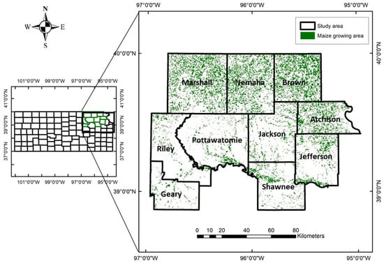
Figure 1.
Study area map consisting of ten rainfed maize-producing counties in northeastern Kansas.
2.2. DSSAT CERES-Maize Cropping System Model
2.2.1. Model Description
The DSSAT CERES-Maize Model v4.8 [43] was used to simulate maize growth in response to the soil, genotype, management, and baseline (1990−2019) and future climate change conditions across the study area. The model requires a variety of soil parameters, including bulk density, organic carbon content, hydraulic conductivity, slope, albedo, color, drainage, the drained upper limit (DUL), lower limit (LL), saturated water content (SAT), and soil texture. Additionally, the model needs inputs for information on cultivars, the environment, and crop management [43]. The planting date and method, seedling depth, plant population, row spacing, cultivar characteristics, tillage type, tillage depth, irrigation method, irrigation amounts and dates, fertilizer application method, fertilizer amount and dates, and harvesting date and method are all necessary crop management parameters. Environmental variables such as daily maximum and minimum temperature, incoming solar radiation, and precipitation are also required as inputs, while dew point temperature and wind speed are optional. A flowchart of steps to simulate baseline (historical) and future maize yields is shown in Figure 2.
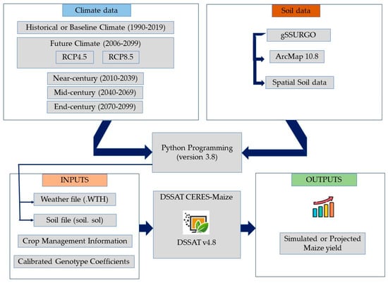
Figure 2.
A flowchart illustrating the process of simulating baseline (historic) and projected yields using the DSSAT CERES-Maize model.
2.2.2. Climate Data
For this study, the baseline (historic) climate data, such as daily maximum and minimum temperatures, precipitation, solar radiation, wind speed, and relative humidity, were obtained from the Gridded Surface Meteorological (gridMET) dataset [44] for 30 years (1990−2019). Future climate data was the output from 18 GCMs (Table 1) from CMIP5 and extracted and statistically downscaled using the Multivariate Adaptative Constructed Analogs (MACAv2) methodology [44]. Each model and experiment aggregated daily maximum and minimum temperature, wind speed, precipitation, relative humidity, and solar radiation from the 4 km downscaled resolution to the county level between 2006 and 2099. The data were formatted in an annual time scale, and three 30-year periods were calculated to represent near (2010−2039), mid (2040−2069), and end (2070−2099) century climate projections. Data were generated for two representative concentration pathways (RCPs), RCP4.5 and RCP8.5, for each GCM. RCPs are widely used in climate change studies to project future greenhouse gas concentrations with the specified radiative forcing pathways under different scenarios of social, economic, and technological development [45]. In RCP4.5, radiative forcing is estimated to increase to approximately 4.5 Wm−2 by 2100 and decline afterward, whereas the RCP8.5 is predicted to have radiative forcing of 8.5 Wm−2 by 2100.

Table 1.
List of global climate models and their source.
Finally, these GCMs data were used as weather inputs in the DSSAT model, creating a multi-model ensemble of 18 models per experiment for each DSSAT treatment. Additionally, mean temperature and precipitation accumulation were calculated under each RCP scenario (near, mid, and end century), and ArcGIS 10.8 [46] was used to map the severity to indicate the changes in temperature and precipitation patterns in the study region.
2.2.3. Soils Data
The Natural resource Conservation Service (NRCS) Gridded Soil Survey Geographic (gSSURGO) database was created for national, regional, and statewide resource planning and analysis of soil data, and provides a 30 m resolution soil data for all counties of the conterminous U.S. [47]. This database contains all the soil properties required for DSSAT, such as sand, silt, and clay percentages, organic carbon content, pH, color, cation exchange capacity, and drainage rate. The soil data development toolbox in ArcMap 10.8 was used to extract the soil information and create the attribute table containing all the required information from various soil depths. The desired soil properties were then exported from the database to Microsoft Excel, which was used as the input for Python [48] to convert these profiles into DSSAT-compatible soil (soil. sol) files.
To obtain the rainfed maize mask for ten selected counties in our study area, a 30 m resolution of the National Agricultural Statistics Service (NASS) Cropland Data Layer (CDL) for the year 2019 was used [49]. We ran the DSSAT model for each soil present in the maize-growing area of each county and created yield maps in ArcMap 10.8 by assigning yield values for each soil.
2.2.4. Crop Management Data
The crop management practices for the DSSAT model simulations were based on recommendations from the Kansas State University’s Research and Extension corn management guide [50]. Rainfed practices were simulated for planting dates ranging from 1 April to 20 May, depending on the location of the county. The plant population was set to 7.6 plants m−2, row spacing was 0.51 m, and 170 kg ha−1 of nitrogen fertilizer was applied as Urea equally divided over two in-season applications (before planting time and during side-dressing and fertigation). To isolate the crop model’s reaction to weather and soil type, only soil and weather variables were allowed to vary from simulation to simulation (Figure 2).
2.2.5. Cultivar Calibration
In the DSSAT CERES-Maize model, yield and phenology are determined by six genetic coefficients (Table 2), and the calibration process attempts to get accurate estimates of these coefficients by comparing simulated and observed data. The model calibration was performed using rainfed crop yield data that was obtained using USDA’s Quickstat 2.0 database [51]. The first step to calibrate the DSSAT model was to adjust the soil fertility factor (SLPF). The soil fertility factor (SLPF), a parameter input linked to variations in soil fertility and soil-based pests, affects the overall growth rate of simulated total biomass by altering daily canopy photosynthesis, and ranges from 0.7 to 1. The default value of SLPF for this study was set to 1, and the value was adjusted manually by checking for the Root Mean Squared Error (RMSE) that gave the least difference between the simulated and observed maize yields. Genotype Coefficient Calculator (GENCALC) was used to calibrate the cultivar parameters with corresponding observations and manually adjusted the remainder of the coefficients [52]. As only maize yield was available for this regional scale study, GENCALC was used to automatically calibrate the cultivar genetic coefficients G2 and G3, and the cultivar phenological coefficients P1, P2, P5, and PHINT were adjusted manually using trial and error, adjusting the values of these coefficients by ±5% to reduce the difference between observed and simulated yields.
Table 2.
Estimated cultivar coefficients for the CERES-Maize model.
Calibrated values of the CERES-Maize model are presented in Table 2. Finally, using the calibrated cultivar, the performance of one dominant soil of each county, three dominant soils per county, and spatially distributed gSSURGO soils were checked.
2.2.6. Model Evaluation and Statistical Analysis
Widely used statistical parameters to assess crop model performance [53,54,55,56] were used for model evaluation and statistical analyses. The following criteria were used to compare simulated and observed data for both calibration and evaluation: RMSE and index of agreement (d) or d-stat [57], given by Equations (1) and (2), respectively:
The lower the RMSE value is, and the closer the value of d-stat is to 1, the better the simulation. In addition, the coefficient of determination (R2) was calculated to evaluate the goodness of fit for the model calibration (i.e., the observed and simulated yield for gSSURGO soils). The coefficient of determination (R2) is considered the most commonly used method for describing the variance between simulated and observed values (Equation (3)). It ranges from 0 to 1, where higher values represent a good model performance, and an R2 > 0.5 is generally considered satisfactory [58].
The Pearson correlation coefficient (r) was used to determine the strength and direction of the linear relationship between the DSSAT projected average maize yield and climatic parameters (growing season average maximum temperature, precipitation and CO2 concentration) under climate change scenarios. Pearson’s correlation coefficient ranges between −1 to 1 [59]. The formula adopted for calculating Pearson’s correlation coefficient is given by Equation (4),
where xi and yi are the values of x and y for the ith individual.
3. Results and Discussion
3.1. DSSAT Performance
The calibration results of the DSSAT–CERES-Maize model for seven years (2000−2006) and for ten counties in the study region showed high accuracy with an RMSE of 1309 kg ha−1 and d-statistics of 0.88 (Figure 3a). The differences between simulated and observed grain yield were no more than 10% of the observations for the calibration period. The model performance during calibration based on end-of-yield followed other studies [60,61] and showed high d-stat values with low RMSE errors between the observed and simulated yield, confirming the fitness of the model for the intended use.
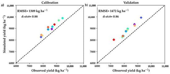
Figure 3.
DSSAT CERES-Maize model (a) calibrated and (b) validated for the ten maize-producing counties of northeastern Kansas.
During the model validation period (five years: 2016−2019), conducted over all ten counties, observed and simulated end-of-season yields matched closely (Figure 3b), with an RMSE of 1472 kg ha−1 and d-statistics of 0.86. The difference between the simulated and observed yield was less than 12% during the validation period. The DSSAT CERES-Maize model overestimated maize yield for almost all simulations, which was expected because the observed yield from the field was limited by weeds and insects, among other factors, that were not considered during the model simulation.
3.2. Impact of Soil Variability on Maize Yield
The number of soils underlying the USDA NASS maize crop mask in each county ranged from 12 to 51, with the largest spatial soil variability in Riley and Pottawatomie County, and the lowest in Jackson County. Pawnee clay loam, Wymore silty clay loam, and Kennebec silt loam were the region’s three most commonly found soils (Figure 4).
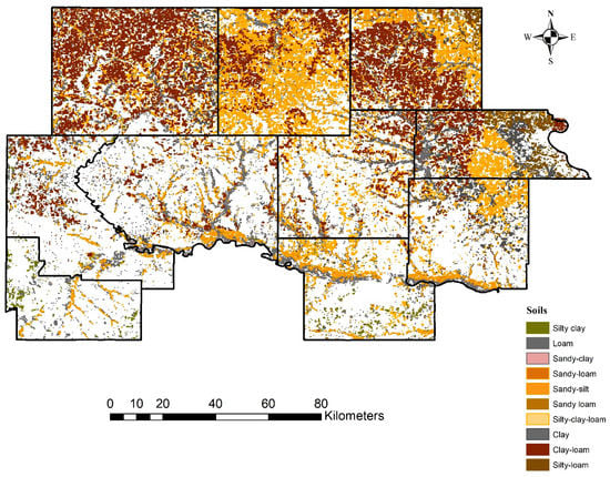
Figure 4.
Spatially distributed gSSURGO soils in the study area. gSSURGO soils were classified based on the soil textural class.
Table 3 shows simulated maize yields that were compared with observed yields for the study region to assess the impact difference in model performance when using the one most common soil of each county, three dominant soils per county, and spatially distributed soils. Under the baseline study period, Brown County was the highest rainfed maize-producing county (9392 kg ha−1), whereas Geary County had the lowest simulated yield (5777 kg ha−1). The average annual yield varied significantly (p < 0.05), and the result reflected that the average simulated yields when using spatially distributed gSSURGO soils were the closest to observed yields in the region compared to simulated yields when using one or three dominant soils for each county. The d-stat for gSSURGO simulations ranged from 0.83 to 0.92, demonstrating the model’s strong capacity to simulate yield under the given conditions with the lowest range of RMSE between 781 to 1326 kg ha−1. Results of correlation analysis showed that the R2 value ranged from 0.63−0.71 for 1 soil, 0.71−0.79 for three soils, and 0.79−0.85 for gSSURGO soils, indicating that the model performed well for the spatially distributed gSSURGO soils and closely mimicked the observed yield (Figure 5).
Table 3.
Average observed and simulated maize yield with d-stat and RMSE for ten counties and various soil types.
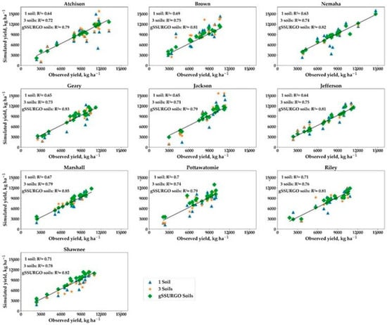
Figure 5.
Comparison between DSSAT-CERES simulated and observed yields for the baseline study period in the top ten maize-producing counties of eastern Kansas while using the one most dominant soil, the three most dominant soils, and spatially distributed gSSURGO soils for each county.
Maize yields ranged from 4222 kg ha−1 to 12261 kg ha−1, with a regional average of 8745 kg ha−1 between soils, and the high-yielding and low-yielding areas were identified in the northeast and southwest part of the study area, respectively (Figure 6). However, there was a large yield variability within the study region due to the spatial distribution of soils. Since soil type, texture, structure, and soil physical, chemical, and engineering properties such as pH, moisture content, and drainage capacity can highly influence crop yields across a field [62,63], there was a significant yield variation observed around the study area even when all other crop management practices remained the same. Since clay loam soil was the dominant soil in this region, and simulated higher yields than other soils, most counties (Atchison, Brown, Nemaha, Marshall, Jackson, Jefferson) showed high-yielding under the baseline study period production (8243−12,261 kg ha−1). On the other hand, sandy loam and sandy silt soils simulated relatively lower yields in this study region, which were dominant in Pottawatomie, Geary, Jackson, and Shawnee counties, yielding maize in the range of 4222−8242 kg ha−1.
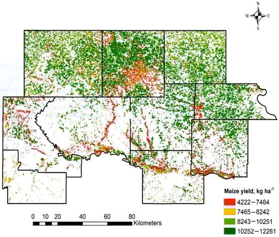
Figure 6.
Variation of maize yield due to the spatial distribution of soils in the ten rainfed maize-producing counties of northeastern Kansas (dark green areas on the map indicate higher simulated maize yields, whereas red color shows areas with extremely low yields).
3.3. Projected Changes in Temperature and Precipitation
Based on the analysis of temperature and precipitation data generated by the 18 GCMs for two RCP scenarios, it was observed that there was an increasing trend in mean temperature with increasing CO2 concentration (Figure 7), whereas the future precipitation values did not follow any specific pattern over the study area. The highest mean temperature recorded at the end of the century under RCP8.5 was 5 °C higher than the 30 years baseline study period (1990−2019). Future precipitation analysis also showed that compared to the baseline period, the study area received less precipitation compared to historic values, and became drier at the end of the century under both RCP scenarios. These results are consistent with some of the other studies that have focused on changes in the climate of the future [64,65,66]. This trend of lower precipitation in the region is probably attributable to extreme heat occurrence as reported in some past studies conducted in the United States [67,68].
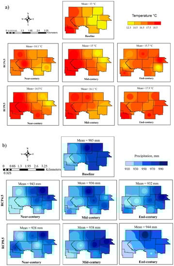
Figure 7.
Spatial distribution of (a) annual mean temperature (°C) and (b) precipitation (mm) obtained from the ensemble mean of 18 GCMs for near-century (2010−2039), mid-century (2040−2069), and end-century (2070−2099) under RCP 4.5 and RCP 8.5 emission scenarios in comparison to the baseline (1990−2019) study period for ten rainfed maize producing counties in northeast Kansas.
3.4. Climate Change Impact on Maize Yield
The impact of changes (with respect to baseline period) in average maximum temperature and total precipitation during the maize growing season in the near, mid, and end of the century under both RCP scenarios affected yield simulations for all future conditions with the highest yield simulated during the near century (2010−2039) under RCP 4.5 scenario and the lowest yield simulated under RCP8.5 at the end of the century (2070−2099) (Table 4).
Table 4.
Summarized average climatic parameters along with average yield under different climate change scenarios during the maize growing season (May–September).
Correlation analysis showed a strong negative correlation between maize yield and temperature (0.96), followed by the CO2 concentration (0.93) (Figure 8), which implies that higher temperature and CO2 concentration tend to adversely impact yields. However, there was a positive correlation between precipitation and maize yield, and the Pearson coefficient was 0.46. So, contrary to the effect of an increase in temperature and CO2 concentration, an increase in precipitation was related to an increase in maize yield. These findings confirm a study by [13] that suggested that high-temperature days with low precipitation conditions during the critical growth stages of maize significantly reduced yield in the United States.
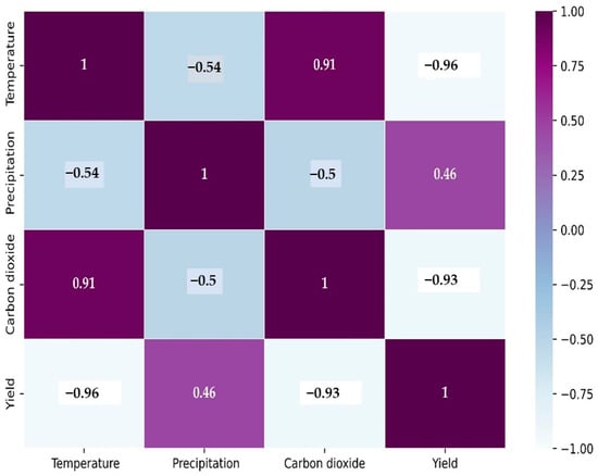
Figure 8.
Pearson correlation coefficient heatmap of maize yield with temperature, precipitation, and CO2 concentration under baseline, near, mid and end century (RCP4.5 and RCP8.5) scenarios.
Figure 9 shows the changes in yield for ten counties of northeastern Kansas by comparing future projected maize yields to baseline yields in terms of a percent difference. A yield loss was observed for the future climate under both the RCP4.5 and RCP8.5 scenarios. All ten counties observed simulated yield loss with the losses ranging from 4−12%, 12−18%, and 22−34%, for RCP 4.5 and 12−19%, 23−27%, and 39−57% under RCP8.5 in the near, mid, and end-century, respectively.
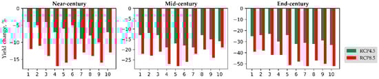
Figure 9.
Percentage yield change in ten maize-producing counties in northeastern Kansas. The number depicted the ten counties of our study area in sequence. 1, Atchison. 2, Brown. 3, Nemaha. 4, Geary. 5, Jackson. 6, Jefferson. 7, Marshall. 8, Pottawatomie. 9, Riley. 10, Shawnee.
It must be noted that higher yield loss was observed under RCP8.5 compared to RCP4.5, which can most likely be explained by high-temperature days, high CO2 concentration levels, and relatively smaller change in precipitation values under the RCP 8.5 emission scenario. High-yield producing counties during the baseline period, such as Atchison, Brown, and Nemaha, exhibited lower yield loss than other counties in the study region under all climate change scenarios. On the other hand, Geary, Jackson, Jefferson, Pottawatomie, and Shawnee counties showed higher yield loss under all climate change scenarios, identifying these as the most vulnerable areas for producing maize in northeastern Kansas. This county-level yield analysis explored the magnitude of yield loss over time and highlighted counties that were relatively less affected by climate change. According to Srivastava et al. (2018), the effects of climate change on maize yield depend on how changes in temperature and precipitation amounts combine to bring about shifts in the onset and length of future growing seasons [69]. Therefore, the decline in precipitation and high-temperature days under future climate tends to lower yields under all climate change scenarios (Figure 9). A finding of a comprehensive study conducted in Africa by Dale et al. (2017) also mentioned that the leading causes of maize yield loss were the high temperatures and changes in precipitation patterns [70].
3.5. Mapping Future Rainfed Maize Yield Variability
Under RCP4.5, in the near, mid, and end centuries, the regional average yields were 7865, 6776, and 6198 kg ha−1, respectively. Under RCP8.5, they were 6985, 5678 and 4744 kg ha−1, respectively. The average yield losses for the entire region under RCP4.5 and RCP8.5 in the near, mid, and end centuries were 7, 16, 28%, and 14, 23, 45%, respectively. The climate change impact was less in the northeastern part of the study region under RCP4.5 for all the study periods (Figure 10). However, under RCP8.5, no specific pattern of yield loss was identified, but the entire region had higher yield loss compared to the RCP4.5 scenarios.
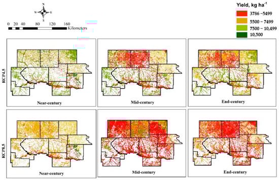
Figure 10.
Yield variation under changing climate in ten maize-producing counties in northeastern Kansas under three study periods (near, mid, and end-century) for RCP4.5 and RCP8.5. The red color stands for low-yielding and the green for the high-yielding region.
4. Conclusions
This study emphasizes that the DSSAT CERES-Maize model can be used to quantify the impacts of climate change along with the spatial soil variability on maize yields. The key findings of this study are that spatial soil variability can impact maize yield and that using spatially distributed soils produces a better simulation of yield as compared to using the most dominant soil in a county. This study concluded under future climate change conditions, northeastern Kansas’ ten top rainfed maize-producing counties would lose substantial maize productivity. Excessively high temperatures, high CO2 concentration levels, and low precipitation associated with future climate would cause a reduction in maize yield in northeastern Kansas. More importantly, this study identifies the vulnerable part of this region under changing climate, which could be a valuable input to develop region-specific adaptation strategies based on quantifying the impact of climate and spatial soil variability on maize yield. The results of this study will be used as a basis for a future study that will include crop suitability analysis. This methodology could be adopted to assess climate change’s impact on other crops across the world.
Author Contributions
Conceptualization, R.S. and V.S.; methodology, R.S. and V.S.; writing—original draft preparation, R.S.; writing—review and editing, R.S., Z.T.Z. and V.S.; supervision, V.S.; project administration, V.S.; funding acquisition, V.S. All authors have read and agreed to the published version of the manuscript.
Funding
This research was supported by the National Science Foundation under award number 2119753.
Institutional Review Board Statement
Not applicable.
Informed Consent Statement
Not applicable.
Data Availability Statement
Not applicable.
Acknowledgments
The authors would like to acknowledge the support of Carl and Melinda Helwig Department of Biological and Agricultural Engineering at Kansas State University, the parent department of co-authors Sen and Sharda.
Conflicts of Interest
The authors declare no conflict of interest.
References
- Reillya, J.; Paltseva, S.; Felzerb, B.; Wanga, X.; Kicklighterb, D.; Melillob, J.; Prinna, R.; Sarofima, M.; Sokolova, A.; Wanga, C. Global economic effects of changes in crops, pasture, and forests due to changing climate, carbon dioxide, and ozone. Energy Policy 2007, 35, 5370–5383. [Google Scholar] [CrossRef]
- Leakey, A.D.B. Rising atmospheric carbon dioxide concentration and the future of C4 crops for food and fuel. Proc. R. Soc. B Biol. Sci. 2009, 276, 2333–2343. [Google Scholar] [CrossRef] [PubMed]
- Rogers, A.; Ainsworth, E.A.; Leakey, A.D. Will elevated carbon dioxide concentration amplify the benefits of nitrogen fixation in legumes? Plant Physiol. 2009, 151, 1009–1016. [Google Scholar] [CrossRef] [PubMed]
- Gornall, J.; Betts, R.; Burke, E.; Clark, R.; Camp, J.; Willett, K.; Wiltshire, A. Implications of climate change for agricultural productivity in the early twenty-first century. Philos. Trans. R. Soc. B Biol. Sci. 2010, 365, 2973–2989. [Google Scholar] [CrossRef] [PubMed]
- Hatfield, J.L.; Dold, C. Climate Impacts on Agriculture: Implications for Crop Production. Agron. J. 2011, 103, 351–370. [Google Scholar] [CrossRef]
- Sen, R.; Karim, N.N.; Islam, M.T.; Adham, A.K.M. Estimation of supplemental irrigation for Aman rice cultivation in Bogra and Dinajpur districts of Bangladesh. Progressive Agriculture. 2017, 28, 42–54. [Google Scholar] [CrossRef]
- Sakurai, G.; Iizumi, T.; Nishimori, M.; Yokozawa. How much has the increase in atmospheric CO2 directly affected past soybean production? Sci. Rep. 2014, 4, 4978. [Google Scholar] [CrossRef]
- Kellogg, W.W. Climate Change and Society: Consequences of Increasing Atmospheric Carbon Dioxide; Routledge: New York, NY, USA, 2019. [Google Scholar] [CrossRef]
- Schauberger, B.; Archontoulis, S.; Arneth, A.; Balkovic, J.; Ciais, P.; Deryng, D.; Frieler, K. Consistent negative response of US crops to high temperatures in observations and crop models. Nat. Commun. 2017, 8, 13931. [Google Scholar] [CrossRef]
- Oduro, C.; Shuoben, B.; Ayugi, B.; Beibei, L.; Babaousmail, H.; Sarfo, I.; Ngoma, H. Observed and Coupled Model Intercomparison Project 6 multimodel simulated changes in near-surface temperature properties over Ghana during the 20th century. Int. J. Clim. 2022, 42, 3681–3701. [Google Scholar] [CrossRef]
- Finger, R. Modeling the sensitivity of agricultural water use to price variability and climate change—An application to Swiss maize production. Agric. Water Manag. 2012, 109, 135–143. [Google Scholar] [CrossRef]
- Wang, M.; Li, Y.; Ye, W.; Bornman, J.F.; Yan, X. Effects of climate change on maize production, and potential adaptation measures: A case study in Jilin Province, China. Clim. Res. 2011, 46, 223–242. [Google Scholar] [CrossRef]
- Sabagh, A.E.; Hossain, A.; Iqbal, M.A.; Barutçular, C.; Islam, M.S.; Çiğ, F.; Saneoka, H. Maize adaptability to heat stress under changing climate. In Plant Stress Physiology; IntechOpen: London, UK, 2020. [Google Scholar]
- USDA National Agricultural Statistics Service, 2019 Census of Agriculture. 2019. Available online: www.nass.usda.gov/AgCensus (accessed on 26 June 2021).
- Ranum, P.; Peña-Rosas, J.P.; Garcia-Casal, M.N. Global maize production, utilization, and consumption. Ann. N. Y. Acad. Sci. 2014, 1312, 105–112. [Google Scholar] [CrossRef] [PubMed]
- Lin, X.; Harrington, J.; Ciampitti, I.; Gowda, P.; Brown, D.; Kisekka, I. Kansas trends and changes in temperature, precipitation, drought, and frost-free days from the 1890s to 2015. J. Contemp. Water Res. Educ. 2017, 162, 18–30. [Google Scholar] [CrossRef]
- Anderson, T.R.; Hawkins, E.; Jones, P.D. CO2, the greenhouse effect and global warming: From the pioneering work of Arrhenius and Callendar to today’s Earth System Models. Endeavour 2016, 40, 178–187. [Google Scholar] [CrossRef]
- Lobell, D.B.; Hammer, G.L.; McLean, G.; Messina, C.; Roberts, M.J.; Schlenker, W. The critical role of extreme heat for maize production in the United States. Nat. Clim. Change 2013, 3, 497–501. [Google Scholar] [CrossRef]
- Asseng, S.; Zhu, Y.; Basso, B.; Wilson, T.; Cammarano, D. Simulation Modeling: Applications in Cropping Systems. In Encyclopedia of Agriculture and Food Systems; Elsevier: Amsterdam, The Netherlands, 2014; pp. 102–112. [Google Scholar] [CrossRef]
- Challinor, A.J.; Watson, J.; Lobell, D.B.; Howden, S.M.; Smith, D.R.; Chhetri, N. A meta-analysis of crop yield under climate change and adaptation. Nat. Clim. Chang. 2014, 4, 287–291. [Google Scholar] [CrossRef]
- Armstrong, R.D.; Fitzpatrick, J.; Rab, M.A.; Abuzar, M.; Fisher, P.D.; O’Leary, G.J. Advances in precision agriculture in south-eastern Australia. III. Interactions between soil properties and water use help explain spatial variability of crop production in the Victorian Mallee. Crop Pasture Sci. 2009, 60, 870–884. [Google Scholar] [CrossRef]
- Sen, R.; Karim, N.N.; Islam, M.T.; Rahman, M.M.; Adham, A.K.M. Estimation of actual crop evapotranspiration and supplemental irrigation for Aman rice cultivation in the northern part of Bangladesh. Fundam. Appl. Agric. 2019, 4, 873–880. [Google Scholar] [CrossRef]
- Milewski, R.; Schmid, T.; Chabrillat, S.; Jiménez, M.; Escribano, P.; Pelayo, M.; Ben-Dor, E. Analyses of the Impact of Soil Conditions and Soil Degradation on Vegetation Vitality and Crop Productivity Based on Airborne Hyperspectral VNIR–SWIR–TIR Data in a Semi-Arid Rainfed Agricultural Area (Camarena, Central Spain). Remote Sens. 2022, 14, 5131. [Google Scholar] [CrossRef]
- Huang, B.; Sun, W.; Zhao, Y.; Zhu, J.; Yang, R.; Zou, Z.; Su, J. Temporal and spatial variability of soil organic matter and total nitrogen in an agricultural ecosystem as affected by farming practices. Geoderma 2007, 139, 336–345. [Google Scholar] [CrossRef]
- Butcher, K.; Wick, A.F.; DeSutter, T.; Chatterjee, A.; Harmon, J. Corn and soybean yield response to salinity influenced by soil texture. Agron. J. 2018, 110, 1243–1253. [Google Scholar] [CrossRef]
- Marschner, P.; Rengel, Z. Nutrient availability in soils. In Marschner’s Mineral Nutrition of Plants; Academic Press: Cambridge, MA, USA, 2023; pp. 499–522. [Google Scholar]
- Schyns, J.F.; Hoekstra, A.Y.; Booij, M.J.; Hogeboom, R.J.; Mekonnen, M.M. Limits to the world’s green water resources for food, feed, fiber, timber, and bioenergy. Proc. Natl. Acad. Sci. USA 2019, 116, 4893–4898. [Google Scholar] [CrossRef] [PubMed]
- Rounsevell, M.D.A.; Annetts, J.E.; Audsley, E.; Mayr, T.; Reginster, I. Modelling the spatial distribution of agricultural land use at the regional scale. Agric. Ecosyst. Environ. 2003, 95, 465–479. [Google Scholar] [CrossRef]
- Amin, A.; Nasim, W.; Mubeen, M.; Nadeem, M.; Ali, L.; Hammad, H.M.; Fathi, A. Optimizing the phosphorus use in cotton by using CSM-CROPGRO-cotton model for semi-arid climate of Vehari-Punjab, Pakistan. Environ. Sci. Pollut. Res. 2017, 24, 5811–5823. [Google Scholar] [CrossRef]
- Jones, J.W.; Hoogenboom, G.; Porter, C.H.; Boote, K.J.; Batchelor, W.D.; Hunt, L.A.; Wilkens, P.W.; Singh, U.; Gijsman, A.J.; Ritchie, J.T. The DSSAT cropping system model. Eur. J. Agron. 2003, 18, 235–265. [Google Scholar] [CrossRef]
- Modala, N.R.; Ale, S.; Rajan, N.; Munster, C.L.; DeLaune, P.B.; Thorp, K.R.; Barnes, E.M. Evaluation of the CSM-CROPGRO-Cotton model for the Texas rolling plains region and simulation of deficit irrigation strategies for increasing water use efficiency. Trans. ASABE 2015, 58, 685–696. [Google Scholar]
- Pathak, T.B.; Fraisse, C.W.; Jones, J.W.; Messina, C.D.; Hoogenboom, G. Use of global sensitivity analysis for CROPGRO cotton model development. Trans. ASABE 2007, 50, 2295–2302. [Google Scholar] [CrossRef]
- Boonwichai, S.; Shrestha, S.; Babel, M.S.; Weesakul, S.; Datta, A. Climate change impacts on irrigation water requirement, crop water productivity and rice yield in the Songkhram River Basin, Thailand. J. Clean. Prod. 2018, 198, 1157–1164. [Google Scholar] [CrossRef]
- Carbone, G.J.; Kiechle, W.; Locke, C.; Mearns, L.O.; McDaniel, L.; Downton, M.W. Response of soybean and sorghum to varying spatial scales of climate change scenarios in the southeastern United States. In Issues in the Impacts of Climate Variability and Change on Agriculture; Springer: Dordrecht, The Netherlands, 2003. [Google Scholar]
- Sarkar, R.; Kar, S. Evaluation of management strategies for sustainable rice–wheat cropping system, using DSSAT seasonal analysis. J. Agric. Sci. 2006, 144, 421–434. [Google Scholar] [CrossRef]
- Yakoub, A.; Lloveras, J.; Biau, A.; Lindquist, J.L.; Lizaso, J.I. Testing and improving the maize models in DSSAT: Development, growth, yield, and N uptake. Field Crops Res. 2017, 212, 95–106. [Google Scholar] [CrossRef]
- Anothai, J.; Patanothai, A.; Jogloy, S.; Pannangpetch, K.; Boote, K.J.; Hoogenboom, G. A sequential approach for determining the cultivar coefficients of peanut lines using end-of-season data of crop performance trials. Field Crops Res. 2008, 108, 169–178. [Google Scholar] [CrossRef]
- Sharda, V.; Handyside, C.; Chaves, B.; McNider, R.T.; Hoogenboom, G. The impact of spatial soil variability on simulation of regional maize yield. Trans. ASABE 2017, 60, 2137–2148. [Google Scholar] [CrossRef]
- Southworth, J.; Pfeifer, R.A.; Habeck, M.; Randolph, J.C.; Doering, O.C.; Johnston, J.J.; Rao, D.G. Changes in soybean yields in the midwestern United States as a result of future changes in climate, climate variability, and CO2 fertilization. Clim. Chang. 2002, 53, 447–475. [Google Scholar] [CrossRef]
- Araya, A.; Kisekka, I.; Gowda, P.H.; Prasad, P.V. Evaluation of water-limited cropping systems in a semi-arid climate using DSSAT-CSM. Agric. Syst. 2017, 150, 86–98. [Google Scholar] [CrossRef]
- Araya, A.; Prasad, P.V.V.; Gowda, P.H.; Sharda, V.; Rice, C.W.; Ciampitti, I.A. Evaluating optimal irrigation strategies for maize in Western Kansas. Agric. Water Manag. 2021, 246, 106677. [Google Scholar] [CrossRef]
- Howard, J.C.; Cakan, E.; Upadhyaya, K. Climate change and its impact on wheat production in Kansas. Int. J. of Food and Agri. Eco. 2016, 4, 1–10. [Google Scholar]
- Hoogenboom, G.; Porter, C.H.; Shelia, V.; Boote, K.J.; Singh, U.; White, J.W.; Pavan, W.; Oliveira, F.A.A.; Moreno-Chain, V.; Lizaso, V.; et al. Decision Support System for Agrotechnology Transfer (DSSAT) Version 4.8 (DSSAT.Net); DSSAT Foundation: Gainesville, FL, USA, 2021. [Google Scholar]
- Abatzoglou, J.T.; Brown, T.J. A comparison of statistical downscaling methods suited for wildfire applications. Int. J. Climatol. 2012, 32, 772–780. [Google Scholar] [CrossRef]
- Taylor, I.H.; Burke, E.; McColl, L.; Falloon, P.; Harris, G.R.; McNeall, D. Contributions to uncertainty in projections of future drought under climate change scenarios. Hydrol. Earth Syst. Sci. Discuss. 2012, 9, 12613–12653. [Google Scholar]
- Ormsby, T.; Napoleon, E.; Burke, R.; Groessl, C.; Bowden, L. Getting to know ArcGIS desktop; Esri Press: Redlands, CA, USA, 2010; p. 592. [Google Scholar]
- Soil Survey Staff. Gridded Soil Survey Geographic (gSSURGO) Database for the United States of America and the Territories, Commonwealths, and Island Nations served by the USDA-NRCS. United States Department of Agriculture, Natural Resources Conservation Service. Available online: https://gdg.sc.egov.usda.gov/ (accessed on 16 November 2020).
- Van Rossum, G.; Drake, F.L., Jr. Python Tutorial; Centrum voor Wiskunde en Informatica: Amsterdam, The Netherlands, 1995. [Google Scholar]
- USDA National Agricultural Statistics Service. Cropland Data Layer; Published Crop-Specific Data Layer [Online]; USDA-NASS: Washington, DC, USA, 2019. Available online: http://nassgeodata.gmu.edu/CropScape/ (accessed on 26 June 2021).
- Ciampitti, I.A.; Correndo, A.; Lancaster, S.; Diaz, D.R.; Aguilar, J.; Sharda, A.; Onofre, R.; McCornack, B. Kansas Corn Management 2023; Kansas State University: Manhattan, KS, USA, 2023. [Google Scholar]
- USDA National Agricultural Statistics Service. Quickstats 2.0; USDA National Agricultural Statistics Service: Washington, DC, USA, 2016. Available online: http://www.nass.usda.gov/Quick_Stats/ (accessed on 16 December 2021).
- Hunt, L.A.; Pararajasingham, S.; Jones, J.W.; Hoogenboom, G.; Imamura, D.T.; Ogoshi, R.M. GENCALC: Software to facilitate the use of crop models for analyzing field experiments. Agron. J. 1993, 85, 1090–1094. [Google Scholar] [CrossRef]
- Bao, S.; Cao, C.; Huang, J.; Ni, X.; Xu, M. Research on yields estimation and yields increasing potential by irrigation of spring maize in Northeast China. In Proceedings of the 2016 IEEE International Geoscience and Remote Sensing Symposium (IGARSS), Beijing, China, 10–15 July 2016; pp. 2506–2509. [Google Scholar]
- Adnan, A.A.; Diels, J.; Jibrin, J.M.; Kamara, A.Y.; Craufurd, P.; Shaibu, A.S.; Tonnang, Z.E.H. Options for calibrating CERES-maize genotype specific parameters under data-scarce environments. PLoS ONE 2019, 14, e0200118. [Google Scholar] [CrossRef]
- Yang, J.M.; Yang, J.Y.; Liu, S.; Hoogenboom, G. An evaluation of the statistical methods for testing the performance of crop models with observed data. Agric. Syst. 2014, 127, 81–89. [Google Scholar] [CrossRef]
- Soler, C.M.T.; Sentelhas, P.C.; Hoogenboom, G. Application of the CSM-CERES-Maize model for planting date evaluation and yield forecasting for maize grown off-season in a subtropical environment. Eur. J. Agron. 2007, 27, 165–177. [Google Scholar] [CrossRef]
- Willmott, C.J. Some Comments on the Evaluation of Model Performance. Bull. Am. Meteorol. Soc. 1982, 63. [Google Scholar] [CrossRef]
- Golmohammadi, G. Development and evaluation of SWATDRAIN, a new model to simulate the hydrology of agricultural tile drained watersheds. Ph.D. Thesis, McGill University, Montreal, QC, Canada, 2014. [Google Scholar]
- Swinscow, T.D.V.; Campbell, M.J. Statistics at Square One; BMJ: London, UK, 2002; pp. 11–25. [Google Scholar]
- Malik, W.; Isla, R.; Dechmi, F. DSSAT-CERES-maize modelling to improve irrigation and nitrogen management practices under Mediterranean conditions. Agric. Water Manag. 2019, 213, 298–308. [Google Scholar] [CrossRef]
- Sharda, V.; Mekonnen, M.M.; Ray, C.; Gowda, P.H. Use of Multiple Environment Variety Trials Data to Simulate Maize Yields in the Ogallala Aquifer Region: A Two Model Approach. JAWRA J. Am. Water Resour. Assoc. 2021, 57, 281–295. [Google Scholar] [CrossRef]
- Plant, R.E. Site-specific management: The application of information technology to crop production. Comput. Electron. Agric. 2001, 30, 9–29. [Google Scholar] [CrossRef]
- Quine, T.A.; Zhang, Y. An investigation of spatial variation in soil erosion, soil properties, and crop production within an agricultural field in Devon, United Kingdom. J. Soil Water Conserv. 2002, 57, 55–65. [Google Scholar]
- Lau, N.C.; Nath, M.J. A model study of heat waves over North America: Meteorological aspects and projections for the twenty-first century. J. Clim. 2012, 25, 4761–4784. [Google Scholar] [CrossRef]
- Argüeso, D.; Di Luca, A.; Perkins-Kirkpatrick, S.E.; Evans, J.P. Seasonal mean temperature changes control future heat waves. Geophys. Res. Lett. 2016, 43, 7653–7660. [Google Scholar] [CrossRef]
- Herring, S.C.; Christidis, N.; Hoell, A.; Kossin, J.P.; Schreck III, C.J.; Stott, P.A. Explaining extreme events of 2016 from a climate perspective. Bull. Am. Meteorol. Soc. 2018, 99, S1–S157. [Google Scholar] [CrossRef]
- Almazroui, M.; Islam, M.N.; Saeed, F.; Saeed, S.; Ismail, M.; Ehsan, M.A.; Barlow, M. Projected changes in temperature and precipitation over the United States, Central America, and the Caribbean in CMIP6 GCMs. Earth Syst. Environ. 2021, 5, 1–24. [Google Scholar] [CrossRef]
- Yue, Y.; Yan, D.; Yue, Q.; Ji, G.; Wang, Z. Future changes in precipitation and temperature over the Yangtze River Basin in China based on CMIP6 GCMs. Atmos. Res. 2021, 264, 105828. [Google Scholar] [CrossRef]
- Srivastava, A.K.; Mboh, C.M.; Zhao, G.; Gaiser, T.; Ewert, F. Climate change impact under alternate realizations of climate scenarios on maize yield and biomass in Ghana. Agric. Syst. 2018, 159, 157–174. [Google Scholar] [CrossRef]
- Dale, A.; Fant, C.; Strzepek, K.; Lickley, M.; Solomon, S. Climate model uncertainty in impact assessments for agriculture: A multi-ensemble case study on maize in sub-Saharan Africa. Earth’s Future 2017, 5, 337–353. [Google Scholar] [CrossRef]


Disclaimer/Publisher’s Note: The statements, opinions and data contained in all publications are solely those of the individual author(s) and contributor(s) and not of MDPI and/or the editor(s). MDPI and/or the editor(s) disclaim responsibility for any injury to people or property resulting from any ideas, methods, instructions or products referred to in the content. |
© 2023 by the authors. Licensee MDPI, Basel, Switzerland. This article is an open access article distributed under the terms and conditions of the Creative Commons Attribution (CC BY) license (https://creativecommons.org/licenses/by/4.0/).