Article

Quantification of Lignosulfonates and Humic Components in Mixtures by ATR FTIR Spectroscopy

by
Evgeniya A. Karpukhina
*,
Dmitry S. Volkov
and
Mikhail A. Proskurnin
Department of Chemistry, Lomonosov Moscow State University, Leninskie Gory 1-3, Moscow 119991, Russia
*
Author to whom correspondence should be addressed.
Agronomy 2023, 13(4), 1141; https://doi.org/10.3390/agronomy13041141
Submission received: 15 March 2023 / Revised: 10 April 2023 / Accepted: 13 April 2023 / Published: 17 April 2023

Abstract

:
The existing techniques for lignosulfonate (LS) in humate fertilizers lack selectivity to humic substances (HS) as the main component; they involve labor- and time-consuming sample preparation to separate the components at the level of detectable LS concentrations. The procedure based on attenuated total reflectance (ATR) FTIR spectroscopy with simple sample preparation for directly quantifying lignosulfonates in aqueous solutions and lignosulfonates and HS in aqueous solutions of preparations based on HS of coal origin (Sigma Aldrich, Powhumus, and Life Force) was developed. Lignosulfonate quantification is possible by exploiting the bands at 1266, 1192, 1093, and 1042 cm−1 with limits of detection of 0.4–2 g/L. Quantifying LS in a mixture with humates includes centrifugation of prepared solutions to separate interfering silicate impurities. LS quantification in the range of 10–100 g/L against HS (up to a 2-fold excess) with an error of up to 5% is possible based on the spectral absorptions at 1093 and 1042 cm−1. Simultaneous quantification of humate in the mixture with an error of up to 10% is possible by exploiting the bands at 1570 and 1383 cm−1 (carboxylates). The study shows the possibility of determining lignosulfonate against an HS background several times higher than lignosulfonate. The developed technique is applicable for analyzing fertilizers of simple composition and quality control of pure humates used for plant growth. Obtaining the most accurate results needs calibration solutions from the same brands that make up the test mixture.

1. Introduction

Lignin and its derivatives have found application in various industries [1]. They are used in the drilling of wells [2], in the production of various types of fuel (briquettes, gas, and boiler fuel) [3,4], and as reducing agents for metals [5] and activated carbon [6,7]. Lignin is a raw material for producing phenol, acetic, and oxalic acids. It is a substitute for sawdust and wood flour in the production of bricks and is used as an additive in asphalt concrete and as a filler for plastics and composites. Lignins are used as sorbents for wastewater, oil products, and heavy metals [7]. They are widespread in agriculture as herbicides and in some fertilizers [8,9]. There are medicinal preparations based on lignin [10,11,12,13]. Lignosulfonates (LS) are lignin derivatives and waste products from the sulfite processing of wood in the pulp and paper industry. About 1.2 million tons of lignosulfonates are produced annually, approximately 10% of the total lignin mass obtained worldwide [14]. LS are widely used; however, their properties differ from the original lignin due to a different structure. Lignosulfonates are surfactants, so they are mainly used as stabilizers, emulsifiers, and dispersants in industries such as oil [15], coal chemicals [16,17], and in the production of building materials [18]. In agriculture, LS are used to treat soil against erosion and plant protection products and fertilizers [19]. In addition, lignosulfonates create solutions resistant to temperature changes and presence of electrolytes [20].
Lignosulfonates have different molecular weights; their formula is not defined, and they have various functional groups. In addition, lignin (and, thus, LS) obtained from various plants differ from each other in chemical composition and structure [21,22]. Currently, no standards regulate the production of lignin and lignosulfonates and how the quality control of the manufactured LS is conducted. Thus, developing relatively prompt and readily reproducible quantification methods for LS is an imperative task.
The assessment of lignin and LS is commonly based on gravimetric analysis after hydrolysis with sulfuric acid, known as the Klason lignin analysis [23,24] or its variants [25,26]. The results of such gravimetric analysis are strongly affected by the presence of components insoluble in lignin, proteins, and fungal chitins. Moreover, this approach does not distinguish between different structures of lignin. Neither method can be considered independent as an analytical method and requires some extra information [23,24]. Dence [27] proposed a non-aqueous potentiometric titration of lignin in tetrabutylammonium hydrochloride in the presence of 4-hydroxybenzoic acid as an internal standard. The advantage is the assessment of hydroxyl groups in lignin and weakly acidic phenolic hydroxyls. In combination with ion exchange, this titrimetric technique is used to quantify strongly acidic (sulfonic) groups in lignosulfonates [28].
UV spectroscopy has been the most widely used technique for lignin and lignosulfonates for several decades. These methods are based on the LS UV absorption at 200–300 nm and are used for LS quantification in sulfite solutions and LS production wastewaters [29]. Spectrophotometric quantification of LS at 280 nm is used for gravel and drilling fluids [30,31]. Since all substances, especially decomposition products of carbohydrates, interfere with the characteristic bands of lignosulfonate, the most critical step of these methods is sample preparation to avoid superimposing the bands of low-molecular substances on LS bands. An approach is lignosulfonate precipitation; e.g., Haars, Lohner and Hüttermann [29] used precipitation with polyethyleneimine. The advantages of this approach are easy repeatability, rapidity, and affordable equipment. However, an additional component is introduced in precipitation techniques, affecting the spectrum. Precipitation and precipitate dissolution also depend on various parameters (temperature, pH, the presence of cations, the sulfonation degree, and LS molecular weight distribution). UV spectrophotometry is also a common method for quantifying acid-soluble lignin [23]. However, if the biomass is not extracted in suitable quantities, foreign extractive materials can complicate the analysis.
Some methods for LS quantification are based on quantitative analysis of the functional groups of its molecules. For the quantification of molecular forms, in most cases, it is necessary to apply more complex mathematical models, e.g., a PCA method for quantification by IR spectroscopy [32,33,34]. There are examples of the quantification of lignin monomers by chromatography [35] and densitometry for lignin and its derivatives, including mixtures [36]; the error in the quantification of lignosulfonate is up to 20%. Combining the latter method with thin-layer chromatography allows the estimation of other components simultaneously with lignin, e.g., monosaccharides [36]. The combination of methods provides the quantification of LS in a mixture without separation. Thus, one of the main tasks of biomass analysis for lignin and LS is to develop an analytical tool for the specific quantification of lignin in absolute amounts, which can simultaneously characterize its structural features in a reliable and high-performance way.
Another relevant task in LS assessment is its quantification in various products and mixtures. This is complicated because LS are additives to complex compositions with many components. One of the most relevant tasks in this aspect is fertilizers and other mixtures based on humic substances (HS). The properties of the final product depend on the HS source, admixtures, and the parameters of the production technology. However, the functions of LS and HS in fertilizers differ, and it is necessary to assess and control the concentrations of each component individually. The concentration of additional components, including lignosulfonates, is usually not controlled. The development of techniques is further complicated because both HS and LS are complex continua of macromolecules of variable composition and irregular structure with different molecular weights. Since humus is formed in nature during lignin decomposition, the structure and properties of HS and LS are similar, and, therefore, quantification methods are the same. As a result, the simultaneous quantification of LS and humates by UV spectroscopy is impossible since humates also absorb in this range [37,38]. The same problem of similar chemical composition arises for densitometric quantification [36]. The potentiometric titration technique also gives false-positive results in lignosulfonate–humate mixtures due to similar functional groups [27]. Lamar, et al. [39] developed a method for the gravimetric quantification of humic and fulvic acids. One of its stages is the adsorption of humates. However, lignosulfonate is also adsorbed, and it becomes impossible to separate humates from LS. Therefore, lignosulfonate additives overestimate the concentration of humic substances in artificial liquid samples [39].
Thus, LS quantification in LS–HS mixtures usually consists of a two-step procedure, first separating lignosulfonates from other components and then assessing the analyte. Extraction with organic solvents is used to separate components, particularly HS [29]. Gel chromatography is often used to isolate lignosulfonates [40]. Most of the efforts are devoted to solving the problem of LS isolation by molecular weight fractions. Sumerskii, et al. [41] described an approach for isolating and purifying LS from a spent sulfite solution. This approach includes sorption on macroreticular nonionic poly(methyl methacrylate) granules (XAD-7 resin) followed by desorption with organic solvents to obtain highly pure lignosulfonates. Similar methods for isolating LS using liquid membranes were used; however, problems arose with the purity of extraction of lignosulfonates, low stability of membranes, and long sample preparation [42].
To sum up, the existing techniques for LS in humate fertilizers lack selectivity to HS as the main component; they involve labor- and time-consuming sample preparation stages to separate the components, and the level of detectable LS concentrations does not entirely fit the task.
IR spectroscopy is already used to characterize the functional group composition of both HS and LS [43,44,45]. We have previously developed a method for directly quantifying HS in fertilizers by IR spectroscopy [46]. However, there are no studies on the quantification of lignosulfonates in mixtures by IR spectroscopy. Furthermore, as HS are present in fertilizers in relatively high concentrations, their solutions have a high IR absorption, preventing IR spectroscopy in the transmission mode. The disadvantages of transmission IR spectroscopy, such as spectral sensitivity to water and the need for specific sample preparation, e.g., pressing into tablets with KBr, are shown as serious for LS quantification [23]. However, ATR FTIR spectroscopy proves suitable for powdered samples and aqueous solutions of complex mixtures, including soil organic matter [47,48,49] and its components [50,51,52,53].
Thus, this work aims to develop a procedure based on ATR FTIR spectroscopy with simple sample preparation for directly quantifying (1) lignosulfonates in aqueous solutions and (2) lignosulfonates and humic substances in aqueous solutions of fertilizer preparations based on humic substances.

2. Materials and Methods

2.1. Samples and Reagents

Commercial samples of humic substances of coal origin were used: humic acid sodium salt (technical grade, Sigma-Aldrich, St. Louis, MO, USA, CAS Number: 68131-04-4), Powhumus (Humintech GmbH, Grevenbroich, Germany, CAS Number: 68514-28-3), and Life Force (Life Force LLC, Saratov, Russia). These samples are further referred to as Aldrich, Powhumus, and Life Force, respectively. Sodium lignosulfonate (Life Force LLC, Saratov, Russia; referred to as LSNa) was used. Water (specific resistance, 18.2 MΩ·cm) from a Milli-Q purification system (Millipore, France) was used throughout.

2.2. IR Equipment and Measurements

IR spectra of dry samples and aqueous solutions were recorded by a Vertex 70 spectrometer (Bruker Optik GmbH, Germany); beamsplitter, KBr; aperture, 8 mm; detector, room temperature DLaTGS; scanner velocity, 10 kHz; sample and background scan numbers, 64, acquisition mode, double-sided, forward–backward. The spectra were recorded in the range 4000–400 cm−1 (2000–800 cm−1 for quantification) with a resolution of 2 cm−1. A GladiATR™ single reflection attenuated total internal reflection accessory with a diamond crystal (Pike Technologies, Madison, WI, USA) was used. A background signal was recorded prior to each sample. The spectrometer and accessory were continuously purged with −70 °C dew point air (a PG28L Purge Gas Generator, PEAK Scientific) at 500 L/h. For aqueous solutions, deionized water was used as a background. A drop of the solution (ca. 30 μL) was placed on the ATR crystal. The sample was in the ambient atmosphere during the measurement, and the environment temperature was kept at 23 ± 1 °C by an air conditioner.
The data was processed using OPUS software (Bruker Optik GmbH 2012, version 7.2.139.1294). All spectra were smoothed over 9 points; ATR correction was performed for the spectra of dry samples (refractive index of sample 1.5 was used). After ATR correction, peak intensity correction was carried out in OPUS software by three types of processing. The correction mode (OPUS notation, Type M “Peak intensity relative to the horizontal baseline”), from now on referred to as Method 1, consisted in drawing a baseline through one set point parallel to the X-axis. The interval of each peak was set, at which the maximum intensity was found, and the peak height relative to the baseline was obtained. In this mode, we used two approaches, (1a) without accounting for the humate concentration and (1b) taking into account the humate concentration for baseline correction. The second type of correction (OPUS notation, Type P “Intensity at the specified frequency”, from now on, Method 2) was to determine the intensity (full peak height) at a given frequency without a baseline. A straight line was constructed for each band by a least-square fit. In the case of Method 1a, the calibration line passes through zero.
We based upon the procedure developed to quantify humic substances in aqueous solutions by ATR FTIR [46] and extended it to aqueous LS–HS solutions. In binary mixtures, the concentration of one component was considered known and used in baseline correction and concentration calculations. Then, the second component was calculated from two equations of the calibration lines (for humate and lignosulfonate). For LS, the intensities of the bands at 1093 and 1042 cm−1; for humate, the intensities of the bands at 1570 and 1383 cm−1 were used. The concentrations of LS and HS for each test band were calculated as, respectively,
c L S = ( I b L S b H S k H S c H S ) / k L S
and
c H S = ( I b L S b H S k L S c L S ) / k H S ,
where I is the band intensity, c H S and c L S are HS and LS concentrations in solution, and coefficients k and b are from individual calibration equations for LS and HS. The values for both wavenumbers corresponding to the same analyte were averaged.
Further data processing was carried out using OriginPro 8.1 software (OriginLab Corp., version 8.1.34.90). The measurement results are presented in accordance with the requirements of ISO/IEC 17025:2005. Coefficients of correlation, confidence limits, standard deviations, relative standard deviations, and limits of detection (LOD) were calculated according to presentation guidelines of IUPAC recommendations 1998 and ISO 5725:1994.

2.3. Other Equipment

Samples were weighed by an Ohaus Discovery DV114C analytical balance (Nänikon, Switzerland; accuracy, 0.0001 g). For quantification, all prepared solutions were centrifuged in 2-mL polypropylene Eppendorf vials in a CM-50 microcentrifuge (ELMI Ltd., Riga, Latvia) at 4000 rpm for 30 min.
Water concentration in samples was measured using an HG63 infrared thermogravimetric moisture analyzer (Mettler–Toledo AG Laboratory & Weighing Technologies, Greifensee, Switzerland). The automatic cut-off criterion “weight loss per unit time” was used; drying ends automatically when the average weight loss (Δm in mg) per unit time (Δt in seconds) falls below the preset value. All amounts and concentrations of humates and sodium lignosulfonate are recalculated for the water concentration.

2.4. Procedures

2.4.1. General Procedure for Solutions

To prepare individual solutions, a weighed portion of the sample was placed in a polypropylene test tube, and 10 mL of water was added and shaken until complete dissolution. To prepare mixture solutions, weighed portions of humate and lignosulfonate were mixed, and then 10 mL of water was added and shaken by hand until complete dissolution.

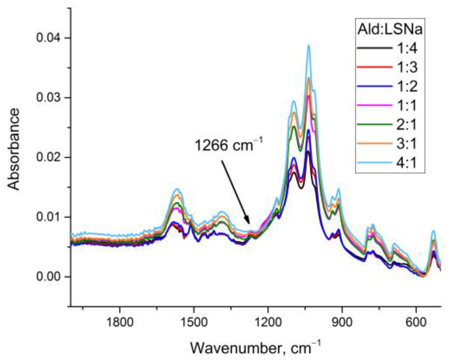
2.4.2. Model Mixtures of Lignosulfonate with Humate for Qualitative Analysis

Solutions of mixtures of lignosulfonate with Aldrich HS were prepared according to Section 2.4.1 with a total concentration of components of 100 g/L and an LS: HS ratio of 1:4, 1:3, 1:2, 1:1, 2:1, 3:1, and 4:1. Further centrifugation of solutions was not performed.

2.4.3. Selection of Conditions for Centrifugation of Humate Solutions for Quantification of Lignosulfonates in the Presence of Humate

An aqueous solution of Powhumus HS with a concentration of 75 g/L was prepared according to Section 2.4.1 and divided into several vials. One vial was left without centrifugation, while the remaining vials were centrifugated at 4000 rpm. After 15, 30, and 60 min, one vial at a time was taken out, and the supernatant liquid was collected into a clean vial and the spectrum of this solution was recorded.

2.4.4. Calibration Solutions of Humate and Lignosulfonate

Individual Powhumus HS and lignosulfonate solutions with concentrations 10, 20, 35, 50, 75, and 100 g/L were prepared according to Section 2.4.1. For mixtures, Powhumus HS was used for calibration and Life Force HS was used to test the technique. For both samples, two series of solutions of lignosulfonate/humate mixtures were prepared according to Section 2.4.1: (1) humate of 20 g/L and LS:HS ratios of 1:2, 1:1, 2:1, and 4:1 and (2) humate of 50 g/L and LS:HS ratios of 1:2, 1:1, 3:2 and 2:1. In all the cases, solutions were centrifugated at 4000 rpm for 30 min. The supernatant liquid was collected into a clean vial, and the spectrum of this solution was recorded.

3. Results and Discussion

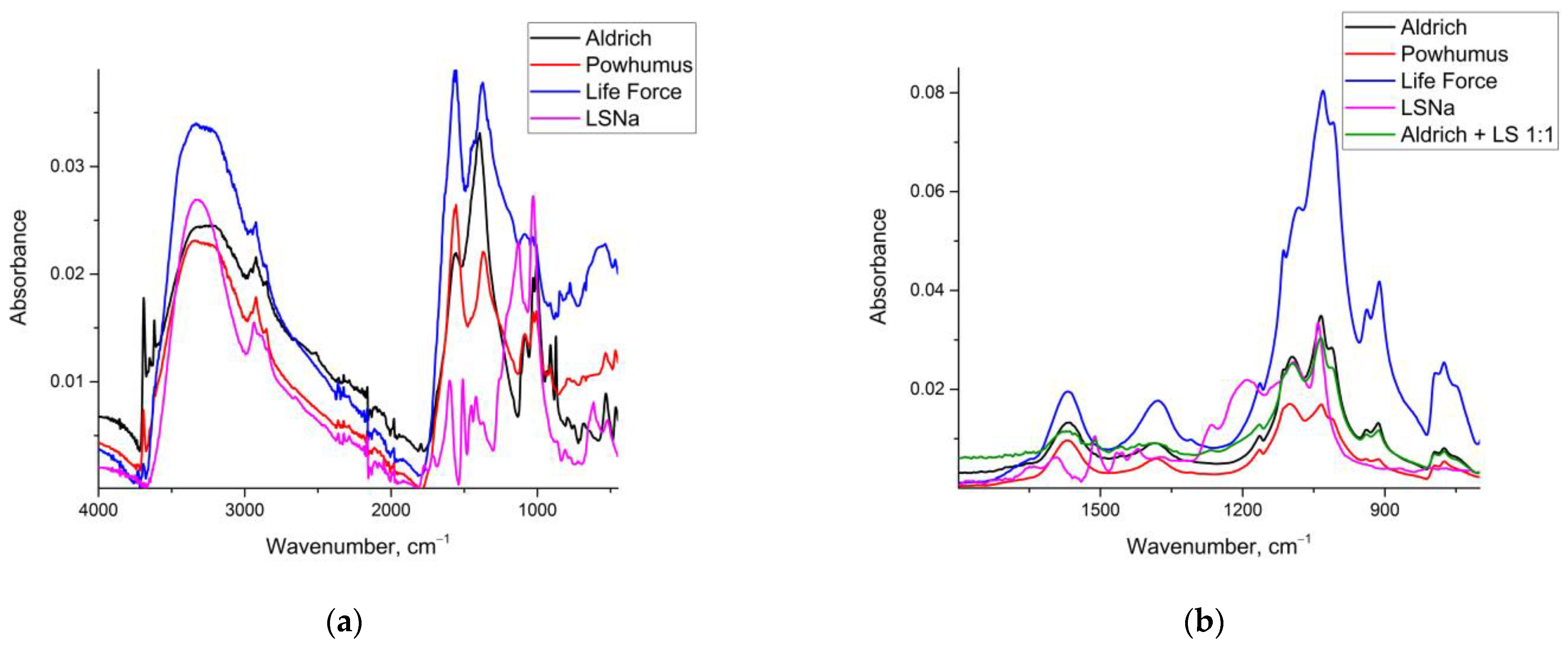
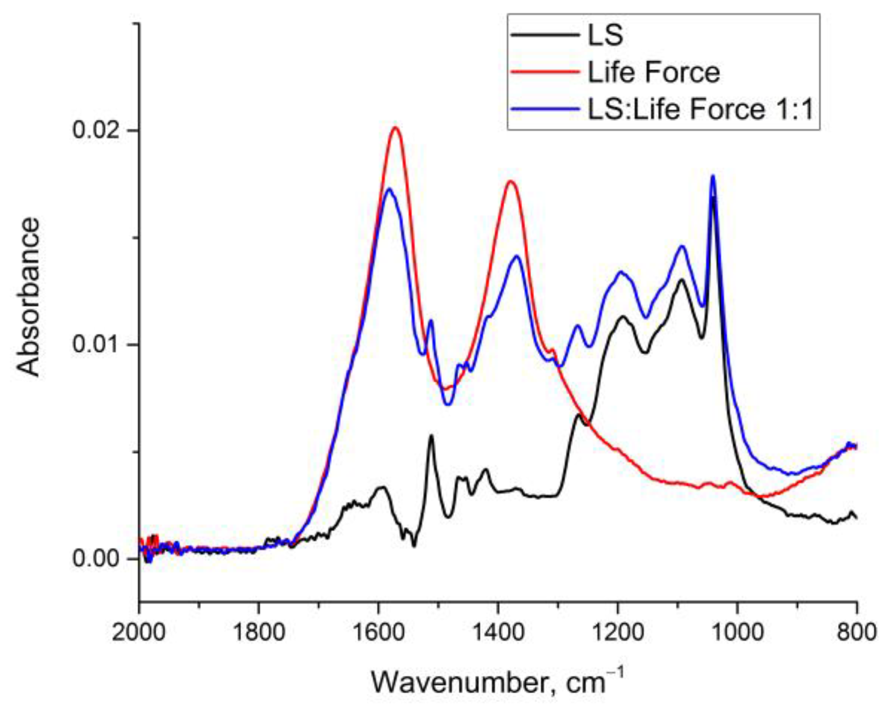
3.1. Band Identification of Humates and Lignosulfonates

ATR-IR spectra of dry individual samples of all brands and their 100 g/L aqueous solutions (Figure 1) were obtained. Based on many sources, the most significant absorption bands of the spectra of lignosulfonate and humates were identified [54,55,56,57,58,59,60,61,62,63,64,65,66]. Table 1 summarizes characteristic bands of lignosulfonate and humates for dry samples and their solutions before and after centrifugation.
The main vibrations characteristic of both humates and LS (Table 1) fall in the ranges 3400–3300, 2935–2850, 1725–1710, 1640–1600, 1570–1560, 1460–1450, 1420–1410, and 1380 cm−1, which correspond to CHx groups, aromatic C=C bonds, quinone and ketone C=O bonds, and carboxyl groups and carboxylate ions [60,67,68,69,70].
Bands at 3690, 1130–1110, 1070, 1035, 1015, 938, 910, and 875 cm−1 are characteristic of HS samples only and correspond to the inorganic, silicate part of humates [46,61,71,72]. The mineral composition of HS is confirmed by elemental analysis [72]. The band at 1070–1050 cm−1 is present in the IR spectra of both compounds. Although in HS, this band most probably corresponds to Si–OH bending vibrations in silicate impurities [46], as it is revealed only in dry HS samples and HS solutions without centrifugation. After centrifugation, the spectra of the humate do not show any of these bands.
Table 1. Absorption bands of dry sodium lignosulfonate (LSNa) and humates (HS) and their aqueous solutions [43,60,61,66,67,68,69,70,71,73,74,75,76,77,78,79,80,81,82].
Wavenumber, cm−1SubstanceAssignment
3691HS *OH stretching of structural hydroxyl groups of SiO2
3400–3300HS, LSNaO–H stretching, N–H stretching (minor), hydrogen-bonded OH; O−H stretching
2935–2925, 2850HS, LSNaC–H stretching of CH2, C−H stretching of −OCH3
1725–1710HS, LSNaasymmetric C=O stretching of –COOH
1640–1600HS, LSNaaromatic C=C skeletal vibrations,
C=O stretching of amide groups (Amide I),
C=O of quinone or H-bonded conjugated ketones,
–COOH group stretch, C–C stretch, aromatic and nonaromatic
1591LSNaaromatic C=C ring breathing
1570–1560HSaromatic C=C skeletal stretching; C=O of quinone or H-bonded conjugated ketones; –COO antisymmetric stretching
1512LSNaaromatic C=C ring breathing
1460–1450HS, LSNaC–H scissoring of CH3 groups
1455LSNaaromatic ring stretching, C–H deformation in –O–CH3 group
1420–1410HS, LSNaaromatic C=C ring breathing, aromatic skeleton vibrations combined with C–H in-plane deformations; O–H deformation and C–O stretching of phenolic OH
1380HS, LSNaWagging C–H of CH2 and CH3 groups, –COO symmetric stretching
1370LSNa,
HS (only dry)
methylene bridge, phenolic OH, C–H wagging in methyl groups
1308HSCO of phenols, CO and OH of carboxylic acids, aliphatic C–C
1266LSNaAr−O stretching breathing, C–O in guaiacyl ring
1192LSNaS=O of SO32−
1130LSNaAr–O stretching breathing
1130–1110HS *C–O stretching of secondary alcohols or ethers
1093LSNaC–O–C and OH of alcohols
1080HS *Si–O stretching
1070–1050HS *, LSNaalcoholic and polysaccharide CO stretch and OH deformation; CO and OH of polysaccharides and alcohols; Si–OH bend in silicates
1042LSNaR–SO3H, OH groups, or S=O stretching
1015HS *Si–O of silicates
938HS *OH deformation of the inner-surface hydroxyl group
910HS *OH deformation of inner hydroxyl groups
875HS *Si–O or Si–O–Si bridge; carbonate; polyaromatic bend vibrations
* in dry samples and solutions without centrifugation.
Although the band at 1308 cm−1 (CO of phenols and CO and OH of carboxylic acids) is characteristic of HS only, it is very weak, and it cannot be used to quantify humate. The bands at 1560 and 1380 cm−1 (carboxylate antisymmetric and symmetric vibrations, respectively) have medium intensities in all the samples. The spectra of all humate brands used in the study have the same set of bands and differ only in the ratio of intensities.
As expected, bands corresponding to sulfonic groups (1192 and 1042 cm−1) are not found in HS samples [43]. Thus, except for carboxylate, no bands in HS spectra correspond to humate organic matter and are present in LS as well.
Spectral features that correspond to lignosulfonates only (Table 1) include bands assigned to aromatic groups at 1591, 1512 (C=C ring breathing), and 1455 cm−1 (most probably aromatic ring stretching vibrations), 1266 and 1130 cm−1 (Ar−O stretching breathing), 1093 cm−1 (C–O–C and OH of alcohols), and sulfonic groups at 1192 and 1042 cm−1 [43,66,67,73,74]. However, the aromatic bands at 1591, 1512, and 1455 cm−1 are weak and located on the intense and broad humate bands, making them unsuitable for quantifying lignosulfonate in mixtures with humate. On the other hand, the band at 1130 cm−1 is weak and appears only in dry lignosulfonate samples. Thus, only the bands at 1266, 1192, 1093, and 1042 cm−1 (interactions between C–O and C–O–H vibrations, S=O, R–SO3–H, OH groups) qualify to be tested for LS quantification [43,60,61,66,67,68,69,70,71,73,74,75,76,77,78,79,80,81,82]. However, these LS characteristic bands cannot be considered pure as they may also correspond to C–O and C–O–H vibrations and because all lignosulfonates have intramolecular interactions that produce intense bands [83] that could entail a possible unavoidable spectral interference from HS. However, intermolecular interactions in humates give rise to vibrations in a broader frequency range and lower intensities [84]; thus, their interference can be considered minor (Figure 1 and Figure 2). Apart from this, the bands at 1266, 1093, and 1042 cm−1 overlap with relatively intense silicate bands, which requires separation of the latter.

3.2. Selection of Quantification Conditions

For calibration solutions, we have selected Powhumus humate. Since Aldrich humate has significant silicate amounts [46], it was used to study the effect of silicates on the qualitative tests and lignosulfonate quantification. The third brand, Life Force, was used to verify the correctness of the procedures. Mixtures of Aldrich humate with lignosulfonate were prepared according to Section 2.4.2 (Figure 2). All the characteristic bands of LS at 1266, 1192, and 1042 cm−1 are clear. The bands of lignosulfonate appear against the background of humate at a concentration level of 10 g/L at a twofold excess of humate. However, significant silicate impurities in humates make it challenging to quantify lignosulfonate as HS silicate peaks at 3691, 1080, 1030, 1015, 938, 910, and 875 cm−1 have high intensities and overlap with most lignosulfonate bands. Thus, without silicate separation, it is possible to detect lignosulfonate only qualitatively by a relatively low-intensity peak in the range of 1265–1270 cm−1 (Figure 2). In addition, the intensity of silicate bands in solution depends on the recording time due to the silicate precipitation [46] and, thus, affects the measurement accuracy.
Therefore, silicates were separated by centrifugation (Section 2.4.3). After centrifugation, the spectrum of HS solutions (Figure 3) reveals no characteristic silicate bands at 3691, 1080, 1030, 1015, 938, 910, and 875 cm−1. Figure 4 shows the spectra of centrifuged solutions of humate, lignosulfonate, and their mixture. In the region of 1300–900 cm−1, free of silicate bands, the bands at 1266, 1093, and 1042 cm−1 are not overlapped by humate bands. Under these conditions, the 1192 cm−1 band (vibrations of C–O–C bonds and OH groups of alcohols) can also be used for LS quantification. The spectra of solutions after 30 and 60 min of centrifugation are identical (Figure 4). Thus, all mixtures for quantification were prepared using centrifugation for 30 min at 4000 rpm.
As mentioned above, the characteristic bands of lignosulfonate at 1266, 1192, and 1042 cm−1 are complex [83] and may overlap with bands of intermolecular interactions in HS. Nevertheless, as lignosulfonates have a more definite functional-group composition and thus give rise to narrower and more intense bands (Figure 1), we can determine LS against the background of humates.

3.3. Band Processing

The bands of the ATR spectra of lignosulfonate solutions are resolved (Figure 1), and band integration does not affect the quantification result. However, peak integration is essential for mixtures of lignosulfonate with humate since the LS and HS bands overlap (Table 1 and Figure 4). Therefore, even though a mixture purified from silicate has no distinct bands in the region of 1300–1000 cm−1, humate still contributes to the total spectrum with broadbands in the entire range and can lead to a significant error in quantifying lignosulfonate. Therefore, when quantifying lignosulfonate, it is strictly necessary to correct it for the background content of HS. Upon preliminary studies, we selected three approaches towards this correction. They are Method 1 (peak intensity relative to horizontal baseline, in two variants) and Method 2, taking into account the humate concentration without a baseline correction (full peak height), Section 2.2.
These calculation methods were compared using the spectra of centrifuged solutions of mixtures of lignosulfonate and Powhumus humate with different component ratios (Table 2). The lignosulfonate concentration was calculated using the bands at 1266, 1192, 1093, and 1042 cm−1 that refer to the spectra of LS only.
In Method 1a, we manually set the boundaries of each peak to calculate the maximum absorption in each range without taking into account the background absorption of the humate. In this case, the straight calibration line passed through zero, and we did not consider the background humate concentration in the further calculation of the LS concentration. This processing resulted in the most significant errors among the tested methods, which are acceptable only for HS concentrations of 20 g/L. The quantification error is positive (overestimation). In Method 1b, in contrast to Method 1a, the second component concentration was taken into account. This approach led to relatively low negative errors for three bands, except for positive errors of 40% for the band of 1042 cm−1. Thus, exploiting the 1093 cm−1 band is possible, which can be used for quantifying lignosulfonate with an error of up to 10% in the studied concentration range.
When using Method 2, we do not draw a baseline and set the peak boundaries but take the absolute intensity value at a given wavelength. This approach gives a minor error in determining the lignosulfonate compared to Method 1b (Table 2) and is suitable for all four LS bands within the specified error range (up to 10%). Thus, the results for all four bands can be compared; the bands at 1266 and 1190 cm−1 give a negative error, and 1090 and 1040 cm−1 give a positive error.
Thus, the selected peak processing method consists of taking the absolute intensity at a given wavelength, while the available background counterpart concentration is considered to minimize the quantification error when calculating the concentration of the test compound. The processing was used in all the subsequent experiments.

3.4. Lignosulfonate Quantification in Neat Solutions

In setting up a procedure for LS in aqueous solutions, we based upon the procedure developed to quantify humic substances in aqueous solutions by ATR FTIR [46]. For all characteristic bands of lignosulfonate, the calibration relationships are linear over the entire LS range of 10–100 g/L (Table 3). As expected, the highest sensitivity (slopes and LODs) among all the characteristic bands of lignosulfonate is achieved for the most intense bands at 1266, 1192, 1093, and 1042 cm−1 that do not overlap with humate bands. The minimum attainable LOD is 0.4 g/L at 1042 cm−1. Therefore, these four bands were selected to quantify lignosulfonate against HS. The quantification error of lignosulfonate in aqueous solutions by these bands does not exceed 3% and, at concentrations below 50 g/L, is lower than 1% (Table 4).

3.5. Lignosulfonate Quantification in Humate Mixtures

For LS quantification against an HS background, mixtures of LS with Powhumus humate centrifuged to separate silicate impurities served as calibration solutions. For bands at 1192 and 1266 cm−1, a quantification error of up to 10% is achievable using the bands at 1192 and 1266 cm−1 for lignosulfonate concentrations above 20 g/L (Table 2; the corresponding error for neat solutions up to 3%, Table 4).
For bands of 1093 and 1042 cm−1, the quantification error does not depend on the LS:HS ratio and HS level (Table 2). These bands provide the most accurate quantification of lignosulfonate with an error of up to 5% in the entire investigated concentration range and at any investigated background humate concentration. For LS concentrations over 75 g/L, an error of even less than 1% is possible, which is comparable to LS quantification from neat solutions (Section 3.4).
We tested this procedure for HS samples different from the humate used to prepare the calibration solutions. The lignosulfonate concentration in the mixture was determined using the calibration for Powhumus humate, while Life Force HS was used to prepare model HS/LS mixtures (Figure 5). The results are presented in Table 5.
All calculated LS concentrations, in this case, were underestimated. The bands at 1266 and 1192 cm−1 give significant quantification errors, more than 15% in the entire range of concentrations and LS:HS ratios. On the contrary, the error by the bands at 1093 and 1042 cm−1 does not exceed 10% for LS concentrations above 40 g/L. At low lignosulfonate concentrations and a 1–2-fold humate excess, the quantification error increased to 20%. At high concentrations of lignosulfonate and its 2-fold excess relative to humate, the error in the most sensitive bands at 1093 and 1042 cm−1 was ca. 10%. Thus, using different humates as the calibration standard, it is possible to determine lignosulfonate in a humate fertilizer with a satisfactory bias.
For a more accurate quantification of lignosulfonate using a humate preparation that is different from the calibration one, it is necessary to calculate the error in determining humate, which can be used to calculate the lignosulfonate content. Indeed, this conclusion works for samples of humates of the same origin. All humates used in this work are of coal origin and produced from leonardite. It is expected that when using humates of a different origin (e.g., peat), the quantification error becomes higher, and the quantification itself may not be possible.
Thus, the procedure for LS quantification in humate fertilizers by ATR FTIR by the bands at 1093 and 1042 cm−1 can be employed in the range of 10–100 g/L and for a 2-fold excess humate concentration with an error of up to 5%. The presence of silicates requires centrifugation of the solutions before measurements.

3.6. Humate Quantification in Lignosulfonate Mixtures

The data obtained for LS makes it possible to estimate the accuracy with which to determine HS against LS. For assessing humate in a mixture with lignosulfonate, the characteristic humate bands at 1570 and 1383 cm−1 were selected, which were previously shown to provide the smallest error in determining humate in solution [46]. For consistency’s sake, the spectra were processed similarly to LS without drawing the baseline and considering the lignosulfonate concentration. The quantification parameters for Powhumus humate are presented in Table 6; the results for model mixtures are summed up in Table 7.
At concentration levels of 20 and 50 g/L, the quantification error is up to 10%. For concentrations of lignosulfonate less than 75 g/L, the quantification error does not exceed 5%. Quantification of HS is possible in the range of 20–180 g/L with an error of 7%; for 50 g/L, with an error of 5%. Thus, even though HS quantification in a mixture with LS is possible with less accuracy than in humate-only solutions [46], an error of 10% is acceptable for most tasks involving LS assessment in humate fertilizers. This conclusion holds true when the humate of the same brand as in the mixture itself is used for the calibration solutions. Simultaneous quantification of LS and HS of different brands requires a more detailed study, which was beyond the scope of this work.
The previously proposed methods did not allow the simultaneous quantification of lignosulfonate and humate in the same mixture without separation; humic substances isolated from the mixture were still contaminated with lignosulfonate, which introduces an error in the quantification of their content, the additionally introduced components influenced the type of the spectrum, and the level of the determined concentrations was limited by the transmission of solutions [28,29,30,39]. The developed technique loosens these limitations and allows simultaneous quantification of humate and lignosulfonate without preliminary separation in highly absorbing solutions (at the level of 10–100 g/L).

4. Conclusions

The study shows the possibility of quantifying lignosulfonate in aqueous solutions against an HS background, which is several times higher than lignosulfonate. It may help regulate LS standard products and quantify LS in humate-based fertilizers. The developed technique is applicable for analyzing fertilizers of simple composition and quality control of pure humates used for plant growth, although with the selected brands of LS and HS at this stage. Obtaining the most accurate results needs calibration solutions from the same brands that make up the test mixture. As LS and HS are chemically complex objects with non-stoichiometric and variable chemical compositions, it is essential not to become constrained to specific brands of LS. Furthermore, humates of coal origin of Life Force, Powhumus, and Aldrich brands were used. As humate fertilizers can be based on HS of various origins, further work needs to check the applicability of the approach for peat and soil humates. It is also feasible to build a chemometric model to quantify LS and HS simultaneously to possibly decrease the error furthermore compared to the values achieved in this study. In addition, fertilizers based on HS often contain other organic and inorganic components, which may significantly complicate their analysis. Therefore, it is necessary to develop methods that make it possible to separate the accompanying components before analysis and quantify HS and LS in multicomponent systems.

Author Contributions

Conceptualization, D.S.V. and M.A.P.; methodology, D.S.V.; software, E.A.K.; validation, E.A.K.; formal analysis, E.A.K.; investigation, E.A.K.; resources, D.S.V.; data curation, E.A.K.; writing—original draft preparation, E.A.K.; writing—review and editing, D.S.V. and M.A.P.; supervision, D.S.V. and M.A.P.; project administration, D.S.V. and M.A.P.; funding acquisition, M.A.P. All authors have read and agreed to the published version of the manuscript.

Funding

This work was supported by The Russian Science Foundation, project number 19-13-00117.

Institutional Review Board Statement

Not applicable.

Informed Consent Statement

Not applicable.

Data Availability Statement

Not applicable.

Acknowledgments

This research was performed according to the Development program of the Interdisciplinary Scientific and Educational School of Lomonosov Moscow State University, “The future of the planet and global environmental change”.

Conflicts of Interest

The authors declare no conflict of interest.

References

  1. Naseem, A.; Tabasum, S.; Zia, K.M.; Zuber, M.; Ali, M.; Noreen, A. Lignin-derivatives based polymers, blends and composites: A review. Int. J. Biol. Macromol. 2016, 93, 296–313. [Google Scholar] [CrossRef] [PubMed]
  2. Adewole, J.K.; Muritala, K.B. Some applications of natural polymeric materials in oilfield operations: A review. J. Pet. Explor. Prod. Technol. 2019, 9, 2297–2307. [Google Scholar] [CrossRef]
  3. Tamilvanan, A. Preparation of Biomass Briquettes using Various Agro-Residues and Waste Papers. J. Biofuels 2013, 4, 47–55. [Google Scholar] [CrossRef]
  4. Berglin, N.; Tomani, P.; Salman, H.; Svärd, S.; Åmand, L.-E. Pilot-scale combustion studies with kraft lignin as a solid biofuel. TAPPI Press Eng. Pulping Environ. Conf. 2008, 2008, 4. [Google Scholar]
  5. Hu, S.; Hsieh, Y.L. Silver nanoparticle synthesis using lignin as reducing and capping agents: A kinetic and mechanistic study. Int. J. Biol. Macromol. 2016, 82, 856–862. [Google Scholar] [CrossRef]
  6. Hayashi, J.i.; Kazehaya, A.; Muroyama, K.; Watkinson, A.P. Preparation of activated carbon from lignin by chemical activation. Carbon 2000, 38, 1873–1878. [Google Scholar] [CrossRef]
  7. Suhas; Carrott, P.J.; Ribeiro Carrott, M.M. Lignin—from natural adsorbent to activated carbon: A review. Bioresour. Technol. 2007, 98, 2301–2312. [Google Scholar] [CrossRef]
  8. Lu, J.; Cheng, M.; Zhao, C.; Li, B.; Peng, H.; Zhang, Y.; Shao, Q.; Hassan, M. Application of lignin in preparation of slow-release fertilizer: Current status and future perspectives. Ind. Crops Prod. 2022, 176, 114267. [Google Scholar] [CrossRef]
  9. Savy, D.; Cozzolino, V. Novel fertilising products from lignin and its derivatives to enhance plant development and increase the sustainability of crop production. J. Clean. Prod. 2022, 366, 132832. [Google Scholar] [CrossRef]
  10. Iravani, S.; Varma, R.S. Greener synthesis of lignin nanoparticles and their applications. Green Chem. 2020, 22, 612–636. [Google Scholar] [CrossRef]
  11. Gao, W.; Kong, F.; Chen, J.; Fatehi, P. Chapter 13—Present and future prospective of lignin-based materials in biomedical fields. In Lignin-Based Materials for Biomedical Applications; Santos, H., Figueiredo, P., Eds.; Elsevier: Amsterdam, The Netherlands, 2021; pp. 395–424. [Google Scholar]
  12. Nan, N.; Hu, W.; Wang, J. Lignin-Based Porous Biomaterials for Medical and Pharmaceutical Applications. Biomedicines 2022, 10, 747. [Google Scholar] [CrossRef]
  13. Ali, D.A.; Mehanna, M.M. Role of lignin-based nanoparticles in anticancer drug delivery and bioimaging: An up-to-date review. Int. J. Biol. Macromol. 2022, 221, 934–953. [Google Scholar] [CrossRef]
  14. Kjellin, M.; Johansson, I. Surfactants from Renewable Resources; Wiley: Hoboken, NJ, USA, 2010. [Google Scholar]
  15. Megiatto, J.D., Jr.; Cerrutti, B.M.; Frollini, E. Sodium lignosulfonate as a renewable stabilizing agent for aqueous alumina suspensions. Int. J. Biol. Macromol. 2016, 82, 927–932. [Google Scholar] [CrossRef] [PubMed]
  16. Hong, N.; Li, Y.; Zeng, W.; Zhang, M.; Peng, X.; Qiu, X. Ultrahigh molecular weight, lignosulfonate-based polymers: Preparation, self-assembly behaviours and dispersion property in coal–water slurry. RSC Adv. 2015, 5, 21588–21595. [Google Scholar] [CrossRef]
  17. Yang, D.; Qiu, X.; Zhou, M.; Lou, H. Properties of sodium lignosulfonate as dispersant of coal water slurry. Energy Convers. Manag. 2007, 48, 2433–2438. [Google Scholar] [CrossRef]
  18. Breilly, D.; Fadlallah, S.; Froidevaux, V.; Colas, A.; Allais, F. Origin and industrial applications of lignosulfonates with a focus on their use as superplasticizers in concrete. Constr. Build. Mater. 2021, 301, 124065. [Google Scholar] [CrossRef]
  19. Pereira, A.d.E.S.; Luiz de Oliveira, J.; Maira Savassa, S.; Barbara Rogério, C.; Araujo de Medeiros, G.; Fraceto, L.F. Lignin nanoparticles: New insights for a sustainable agriculture. J. Clean. Prod. 2022, 345, 131145. [Google Scholar] [CrossRef]
  20. Garguiak, J.D.; Lebo, S.E. Commercial Use of Lignin-Based Materials. In Lignin: Historical, Biological, and Materials Perspectives; ACS Symposium Series; American Chemical Society: Washington, DC, USA, 1999; Volume 742, pp. 304–320. [Google Scholar]
  21. Zhang, T.; Yang, Y.L.; Liu, S.Y. Application of biomass by-product lignin stabilized soils as sustainable Geomaterials: A review. Sci. Total. Environ. 2020, 728, 138830. [Google Scholar] [CrossRef] [PubMed]
  22. Novák, F.; Šestauberová, M.; Hrabal, R. Structural features of lignohumic acids. J. Mol. Struct. 2015, 1093, 179–185. [Google Scholar] [CrossRef]
  23. Lupoi, J.S.; Singh, S.; Parthasarathi, R.; Simmons, B.A.; Henry, R.J. Recent innovations in analytical methods for the qualitative and quantitative assessment of lignin. Renew. Sustain. Energy Rev. 2015, 49, 871–906. [Google Scholar] [CrossRef]
  24. van Erven, G.; de Visser, R.; Merkx, D.W.H.; Strolenberg, W.; de Gijsel, P.; Gruppen, H.; Kabel, M.A. Quantification of Lignin and Its Structural Features in Plant Biomass Using 13C Lignin as Internal Standard for Pyrolysis-GC-SIM-MS. Anal. Chem. 2017, 89, 10907–10916. [Google Scholar] [CrossRef] [PubMed]
  25. Sluiter, J.B.; Ruiz, R.O.; Scarlata, C.J.; Sluiter, A.D.; Templeton, D.W. Compositional Analysis of Lignocellulosic Feedstocks. 1. Review and Description of Methods. J. Agric. Food Chem. 2010, 58, 9043–9053. [Google Scholar] [CrossRef]
  26. Fukushima, R. Can Lignin Be Accurately Measured? Crop. Sci. 2005, 45, 832–839. [Google Scholar] [CrossRef]
  27. Dence, C.W. Determination of Carboxyl Groups. In Methods in Lignin Chemistry; Lin, S.Y., Dence, C.W., Eds.; Springer Series in Wood Science; Springer: Berlin/Heidelberg, Germany, 1992; pp. 458–464. [Google Scholar]
  28. El Mansouri, N.-E.; Salvadó, J. Analytical methods for determining functional groups in various technical lignins. Ind. Crops Prod. 2007, 26, 116–124. [Google Scholar] [CrossRef]
  29. Haars, A.; Lohner, S.; Hüttermann, A. Quantitative Determination of Lignosulfonates from Sulfite Spend Liquors Using Precipitation with Polyethyleneimine. Holzforschung 1981, 35, 59–66. [Google Scholar] [CrossRef]
  30. Carney, L.L.; Skelly, W.G.; Gullickson, R. Quantitative Determination Of Lignosulfonates in Drilling Fluids By Ultraviolet Absorption Analysis. J. Pet. Technol. 1972, 24, 651–656. [Google Scholar] [CrossRef]
  31. Edvardsson, K.; Ekblad, J.; Magnusson, R. Methods for Quantification of Lignosulphonate and Chloride in Gravel Wearing Courses. Road Mater. Pavement Des. 2011, 11, 171–185. [Google Scholar] [CrossRef]
  32. Lucarini, M.; Durazzo, A.; Kiefer, J.; Santini, A.; Lombardi-Boccia, G.; Souto, E.B.; Romani, A.; Lampe, A.; Ferrari Nicoli, S.; Gabrielli, P.; et al. Grape Seeds: Chromatographic Profile of Fatty Acids and Phenolic Compounds and Qualitative Analysis by FTIR-ATR Spectroscopy. Foods 2020, 9, 10. [Google Scholar] [CrossRef]
  33. Allison, G.G.; Thain, S.C.; Morris, P.; Morris, C.; Hawkins, S.; Hauck, B.; Barraclough, T.; Yates, N.; Shield, I.; Bridgwater, A.V.; et al. Quantification of hydroxycinnamic acids and lignin in perennial forage and energy grasses by Fourier-transform infrared spectroscopy and partial least squares regression. Bioresour. Technol. 2009, 100, 1252–1261. [Google Scholar] [CrossRef]
  34. Tamaki, Y.; Mazza, G. Rapid Determination of Lignin Content of Straw Using Fourier Transform Mid-Infrared Spectroscopy. J. Agric. Food Chem. 2011, 59, 504–512. [Google Scholar] [CrossRef] [PubMed]
  35. Dao Thi, H.; Van Aelst, K.; Van den Bosch, S.; Katahira, R.; Beckham, G.T.; Sels, B.F.; Van Geem, K.M. Identification and quantification of lignin monomers and oligomers from reductive catalytic fractionation of pine wood with GC × GC FID/MS. Green Chem. 2022, 24, 191–206. [Google Scholar] [CrossRef]
  36. Khaliliyan, H.; Schuster, C.; Sumerskii, I.; Guggenberger, M.; Oberlerchner, J.T.; Rosenau, T.; Potthast, A.; Böhmdorfer, S. Direct Quantification of Lignin in Liquors by High Performance Thin Layer Chromatography-Densitometry and Multivariate Calibration. ACS Sustain. Chem. Eng. 2020, 8, 16766–16774. [Google Scholar] [CrossRef]
  37. Kumada, K. Chapter 3 Spectroscopic Characteristics of Humic Acids and Fulvic Acids. In Chemistry of Soil Organic Matter; Developments in Soil Science; Elsevier: Amsterdam, The Netherlands, 1987; Volume 17, pp. 34–56. [Google Scholar]
  38. Giovanela, M.; Crespo, J.S.; Antunes, M.; Adamatti, D.S.; Fernandes, A.N.; Barison, A.; da Silva, C.W.P.; Guégan, R.; Motelica-Heino, M.; Sierra, M.M.D. Chemical and spectroscopic characterization of humic acids extracted from the bottom sediments of a Brazilian subtropical microbasin. J. Mol. Struct. 2010, 981, 111–119. [Google Scholar] [CrossRef]
  39. Lamar, R.T.; Olk, D.C.; Mayhew, L.; Bloom, P.R. A new standardized method for quantification of humic and fulvic acids in humic ores and commercial products. J. AOAC Int. 2014, 97, 721–730. [Google Scholar] [CrossRef]
  40. Ouyang, X.P.; Zhang, P.; Tan, C.M.; Deng, Y.H.; Yang, D.J.; Qiu, X.Q. Isolation of lignosulfonate with low polydispersity index. Chin. Chem. Lett. 2010, 21, 1479–1481. [Google Scholar] [CrossRef]
  41. Sumerskii, I.; Korntner, P.; Zinovyev, G.; Rosenau, T.; Potthast, A. Fast track for quantitative isolation of lignosulfonates from spent sulfite liquors. RSC Adv. 2015, 5, 92732–92742. [Google Scholar] [CrossRef]
  42. Chakrabarty, K.; Krishna, K.V.; Saha, P.; Ghoshal, A.K. Extraction and recovery of lignosulfonate from its aqueous solution using bulk liquid membrane. J. Membr. Sci. 2009, 330, 135–144. [Google Scholar] [CrossRef]
  43. Zhou, H.; Yang, D.; Zhu, J.Y. Molecular Structure of Sodium Lignosulfonate from Different Sources and their Properties as Dispersant of TiO2Slurry. J. Dispers. Sci. Technol. 2015, 37, 296–303. [Google Scholar] [CrossRef]
  44. Li, P.-Q.; Lu, J.; Yang, R.; Liu, Y.-J. Comparison of structures and properties of lignosulfonate in different pulping waste liquors. In Advanced Materials and Energy Sustainability; World Scientific: Singapore, 2017. [Google Scholar]
  45. Volkov, D.; Rogova, O.; Proskurnin, M. Temperature Dependences of IR Spectra of Humic Substances of Brown Coal. Agronomy 2021, 11, 1822. [Google Scholar] [CrossRef]
  46. Karpukhina, E.; Mikheev, I.; Perminova, I.; Volkov, D.; Proskurnin, M. Rapid quantification of humic components in concentrated humate fertilizer solutions by FTIR spectroscopy. J. Soils Sed. 2018, 19, 2729–2739. [Google Scholar] [CrossRef]
  47. Artz, R.R.E.; Chapman, S.J.; Jean Robertson, A.H.; Potts, J.M.; Laggoun-Défarge, F.; Gogo, S.; Comont, L.; Disnar, J.-R.; Francez, A.-J. FTIR spectroscopy can be used as a screening tool for organic matter quality in regenerating cutover peatlands. Soil Biol. Biochem. 2008, 40, 515–527. [Google Scholar] [CrossRef]
  48. Artz, R.; Chapman, S.; Campbell, C. Substrate utilisation profiles of microbial communities in peat are depth dependent and correlate with whole soil FTIR profiles. Soil Biol. Biochem. 2006, 38, 2958–2962. [Google Scholar] [CrossRef]
  49. Fernandes, A.N.; Giovanela, M.; Esteves, V.I.; Sierra, M.M.d.S. Elemental and spectral properties of peat and soil samples and their respective humic substances. J. Mol. Struct. 2010, 971, 33–38. [Google Scholar] [CrossRef]
  50. Xing, Z.; Tian, K.; Du, C.; Li, C.; Zhou, J.; Chen, Z. Agricultural soil characterization by FTIR spectroscopy at micrometer scales: Depth profiling by photoacoustic spectroscopy. Geoderma 2019, 335, 94–103. [Google Scholar] [CrossRef]
  51. Vaudour, E.; Cerovic, Z.G.; Ebengo, D.M.; Latouche, G. Predicting Key Agronomic Soil Properties with UV-Vis Fluorescence Measurements Combined with Vis-NIR-SWIR Reflectance Spectroscopy: A Farm-Scale Study in a Mediterranean Viticultural Agroecosystem. Sensors 2018, 18, 1157. [Google Scholar] [CrossRef]
  52. Yeasmin, S.; Singh, B.; Johnston, C.T.; Sparks, D.L. Organic carbon characteristics in density fractions of soils with contrasting mineralogies. Geochim. Cosmochim. Acta 2017, 218, 215–236. [Google Scholar] [CrossRef]
  53. Raphael, L. Application of FTIR Spectroscopy to Agricultural Soils Analysis. In Fourier Transforms—New Analytical Approaches and FTIR Strategies; Nikolic, G., Ed.; InTech: London, UK, 2011; pp. 385–404. [Google Scholar]
  54. Stevenson, F.J.; Goh, K.M. Infrared spectra of humic acids and related substances. Geochim. Cosmochim. Acta 1971, 35, 471–483. [Google Scholar] [CrossRef]
  55. MacCarthy, P.; Mark, H.B.; Griffiths, P.R. Direct measurement of the infrared spectra of humic substances in water by Fourier transform infrared spectroscopy. J. Agric. Food Chem. 2002, 23, 600–602. [Google Scholar] [CrossRef]
  56. Baes, A.U.; Bloom, P.R. Diffuse Reflectance and Transmission Fourier Transform Infrared (DRIFT) Spectroscopy of Humic and Fulvic Acids. Soil Sci. Soc. Am. J. 1989, 53, 695–700. [Google Scholar] [CrossRef]
  57. Morra, M.J.; Marshall, D.B.; Lee, C.M. FT-IR analysis of aldrich humic acid in water using cylindrical internal reflectance. Commun. Soil Sci. Plant Anal. 2008, 20, 851–867. [Google Scholar] [CrossRef]
  58. Senesi, N.; Miano, T.M.; Provenzano, M.R.; Brunetti, G. Spectroscopic and compositional comparative characterization of I.H.S.S. reference and standard fulvic and humic acids of various origin. Sci. Total Environ. 1989, 81, 143–156. [Google Scholar] [CrossRef]
  59. Lynch, B.M.; Smith-Palmer, T. Interpretation of FTIR spectral features in the 1000-1200 cm−1 region in humic acids—Contributions from particulate silica in different sampling media. Can. J. Appl. Spectrosc. 1992, 37, 126–131. [Google Scholar]
  60. Orlov, D.S. Humic Substances of Soils and General Theory of Humification; Taylor & Francis: New York, NY, USA, 1995. [Google Scholar]
  61. Madejová, J. Baseline Studies of the Clay Minerals Society Source Clays: Infrared Methods. Clay Clay Min. 2001, 49, 410–432. [Google Scholar] [CrossRef]
  62. Ribeiro, J.S.; Ok, S.S.; Garrigues, S.; de la Guardia, M. Ftir Tentative Characterization of Humic Acids Extracted from Organic Materials. Spectr. Lett. 2001, 34, 179–190. [Google Scholar] [CrossRef]
  63. Tanaka, T.; Nagao, S.; Ogawa, H. Attenuated Total Reflection Fourier Transform Infrared (ATR-FTIR) Spectroscopy of Functional Groups of Humic Acid Dissolving in Aqueous Solution. Anal. Sci. Suppl. 2002, 17, i1081–i1084. [Google Scholar] [CrossRef]
  64. Palamarchuk, I.; Brovko, O.; Bogolitsyn, K.; Boitsova, T.; Ladesov, A.; Ivakhnov, A. Relationship of the structure and ion-exchange properties of polyelectrolyte complexes based on biopolymers. Russ. J. Appl. Chem. 2015, 88, 103–109. [Google Scholar] [CrossRef]
  65. Farad, S.; Manan, M.A.; Ismail, N.; Nsamba, H.K.; Galiwango, E.; Kabenge, I. Formulation of Surfactants from Coconut Coir Containing Lignosulfonate for Surfactant-Polymer Flooding; The National Research Repository of Uganda: Kampala, Uganda, 2016. [Google Scholar]
  66. Xu, H.; Yu, G.; Mu, X.; Zhang, C.; DeRoussel, P.; Liu, C.; Li, B.; Wang, H. Effect and characterization of sodium lignosulfonate on alkali pretreatment for enhancing enzymatic saccharification of corn stover. Ind. Crops Prod. 2015, 76, 638–646. [Google Scholar] [CrossRef]
  67. Ertani, A.; Francioso, O.; Tugnoli, V.; Righi, V.; Nardi, S. Effect of commercial lignosulfonate-humate on Zea mays L. metabolism. J. Agric. Food Chem. 2011, 59, 11940–11948. [Google Scholar] [CrossRef]
  68. Hejzlar, J.; Szpakowska, B.; Wershaw, R.L. Comparison of humic substances isolated from peatbog water by sorption on DEAE-cellulose and amberlite XAD-2. Water Res. 1994, 28, 1961–1970. [Google Scholar] [CrossRef]
  69. Stevenson, F.J. Humus Chemistry: Genesis, Composition, Reactions, Second Edition (Stevenson, F.J.). J. Chem. Educ. 1995, 72, A93. [Google Scholar] [CrossRef]
  70. Senesi, N.; D’Orazio, V.; Ricca, G. Humic acids in the first generation of EUROSOILS. Geoderma 2003, 116, 325–344. [Google Scholar] [CrossRef]
  71. Madejová, J. FTIR techniques in clay mineral studies. Vib. Spectrosc. 2003, 31, 1–10. [Google Scholar] [CrossRef]
  72. Karpukhina, E.A.; Vlasova, E.A.; Volkov, D.S.; Proskurnin, M.A. Comparative Study of Sample-Preparation Techniques for Quantitative Analysis of the Mineral Composition of Humic Substances by Inductively Coupled Plasma Atomic Emission Spectroscopy. Agronomy 2021, 11, 2453. [Google Scholar] [CrossRef]
  73. Li, B.; Ouyang, X.P. Structure and Properties of Lignosulfonate with Different Molecular Weight Isolated by Gel Column Chromatography. Adv. Mater. Res. 2012, 554, 2024–2030. [Google Scholar] [CrossRef]
  74. Han, H.; Li, J.; Wang, H.; Han, Y.; Chen, Y.; Li, J.; Zhang, Y.; Wang, Y.; Wang, B. One-Step Valorization of Calcium Lignosulfonate To Produce Phenolics with the Addition of Solid Base Oxides in the Hydrothermal Reaction System. Energy Fuels 2019, 33, 4302–4309. [Google Scholar] [CrossRef]
  75. Anas, A.K.; Prakoso, N.I.; Sasvita, D. The Initial Comparison Study of Sodium Lignosulfonate, Sodium Dodecyl Benzene Sulfonate, and Sodium p-Toluene Sulfonate Surfactant for Enhanced Oil Recovery. IOP Conf. Ser. Mater. Sci. Eng. 2018, 349, 012005. [Google Scholar] [CrossRef]
  76. Chen, R.; Wu, Q. Modified lignosulfonate as adhesive. J. Appl. Polym. Sci. 1994, 52, 437–443. [Google Scholar] [CrossRef]
  77. Mansouri, N.; Yuan, Q.; Huang, F. Characterization of alkaline lignins for use in penol-formaldehyde and epoxy resins. Bioresources 2011, 6, 2647–2662. [Google Scholar] [CrossRef]
  78. Lucas, S.; Tognonvi, M.T.; Gelet, J.L.; Soro, J.; Rossignol, S. Interactions between silica sand and sodium silicate solution during consolidation process. J. Non Cryst. Solids 2011, 357, 1310–1318. [Google Scholar] [CrossRef]
  79. Bleken, B.T.; Mino, L.; Giordanino, F.; Beato, P.; Svelle, S.; Lillerud, K.P.; Bordiga, S. Probing the surface of nanosheet H-ZSM-5 with FTIR spectroscopy. Phys. Chem. Chem. Phys. 2013, 15, 13363–13370. [Google Scholar] [CrossRef]
  80. Russell, J.D.; Fraser, A.R. Infrared methods. In Clay Mineralogy: Spectroscopic and Chemical Determinative Methods; Wilson, M.J., Ed.; Springer: Dordrecht, The Netherlands, 1994; pp. 11–67. [Google Scholar]
  81. De Benedetto, G.E.; Laviano, R.; Sabbatini, L.; Zambonin, P.G. Infrared spectroscopy in the mineralogical characterization of ancient pottery. J. Cult. Herit. 2002, 3, 177–186. [Google Scholar] [CrossRef]
  82. Roeges, N.P.G. A Guide to the Complete Interpretation of Infrared Spectral of Organic Structures; Wiley: Hoboken, NJ, USA, 1994. [Google Scholar]
  83. Kubo, S.; Kadla, J.F. Hydrogen bonding in lignin: A Fourier transform infrared model compound study. Biomacromolecules 2005, 6, 2815–2821. [Google Scholar] [CrossRef] [PubMed]
  84. Sutton, R.; Sposito, G. Molecular structure in soil humic substances: The new view. Environ. Sci Technol 2005, 39, 9009–9015. [Google Scholar] [CrossRef] [PubMed]
Figure 1. ATR absorption spectra of (a) lignosulfonate and humate powders from Aldrich, Powhumus, and Life Force in the mid-IR region (4000–500 cm−1) and (b) aqueous solutions of lignosulfonate and the same humates, and a mixture of Aldrich with lignosulfonate in the mid-IR region (1800–700 cm−1).
Agronomy 13 01141 g001
Figure 2. ATR absorption spectra of aqueous solutions of Aldrich HS and LSNa mixtures of different compositions (total concentration of components, 100 g/L) in the range of 2000–500 cm−1.
Agronomy 13 01141 g002
Figure 3. ATR spectra of an aqueous solution of Powhumus humate with a concentration of 75 g/L before and after 15, 30, and 60 min of centrifugation.
Agronomy 13 01141 g003
Figure 4. ATR absorption spectra of centrifuged aqueous solutions of sodium lignosulfonate, potassium humate Powhumus (Pow), and their 1:1 mixture, with concentrations of 50 g/L.
Agronomy 13 01141 g004
Figure 5. ATR absorption spectra of centrifuged aqueous solutions of sodium lignosulfonate, sodium humate Life Force, and their 1:1 mixture.
Agronomy 13 01141 g005
Table 2. Concentrations and the error of lignosulfonate quantification in mixtures with Powhumus humate by the bands at 1266, 1192, 1093, and 1042 cm−1 by different peak processing methods (n = 6, p = 0.95).
Added, g/LMethod 1a Method 1b Method 2
LSNaPowhumus126611921093104212661192109310421266119210931042
Found LS, g/L
1020241515165.06.59.2147.78.31010
2020322425301315192817182121
4020544547563637405638384141
802091848910974768011176788081
2550613937421719253523232625
5050856364754143507046475151
7550109879010866687510471717676
1005013211111614089921001389496100101
Error, %
1020140534663−50−35−839−23−171.30.2
202062202649−33−23−341−13−1045
402035131841−11−80.440−5−421.6
80201451136−8−5−0.239−5−30.50.9
2550146554866−31−26−0.440−9−931.3
505070262749−18−140.639−8−61.51.3
755046162043−12−100.739−6−511
1005032111640−11−80.138−6−40.50.7
Table 3. Parameters for the quantification of sodium lignosulfonate (n = 6, p = 0.95).
Wavenumber, cm−1Slope, L/g × 105Correlation CoefficientLOD, g/L
16423.7 ± 0.20.98985
15915.8 ± 0.30.99743
15129.5 ± 0.30.99914
14666.7 ± 0.20.99924
14556.7 ± 0.20.99865
14207.3 ± 0.10.99944
126612.3 ± 0.50.99982
119221.4 ± 0.60.99991
109325.1 ± 0.60.99990.5
104232.5 ± 0.70.99990.4
Table 4. Error in determining lignosulfonate in neat solutions (n = 6, p = 0.95).
Added LS, g/LError of Calculation of LS Concentration, g/L
1266 cm−11192 cm−11093 cm−11042 cm−1
20−3.0−3.0−1.01.0
500.1−0.10.60.7
100−0.7−0.50.020.8
Table 5. Concentrations and errors of lignosulfonate quantification in mixtures with Life Force humate using a calibration by Powhumus at different bands (n = 6, p = 0.95).
Added, g/LFound, g/L
LSNaLife Force1266 cm−11192 cm−11093 cm−11042 cm−1
Found, g/L
10205.16.48.08.2
202015161818
402032343737
802068717575
255019202222
505042424546
755059646969
1005074839091
Error, %
1020−49−36−20−18
2020−24−21−12−11
4020−20−15−8−8
8020−15−11−6−6
2550−24−21−14−14
5050−15−15−9−9
7550−21−15−9−8
10050−26−17−10−9
Table 6. Quantification of humate (Powhumus) by the bands 1560 and 1383 cm−1 without baseline correction (n = 10, p = 0.95).
Wavenumber, cm−1Slope, L/g × 105Correlation CoefficientLODs, g/L
15702.9 ± 0.10.98230.7
13835.8 ± 0.40.99841
Table 7. The error of humate quantification in the mixtures with lignosulfonate by the characteristic bands of both humate and lignosulfonate.
Added, g/L1570 cm−11383 cm−1
PowhumusLSNa
Found, g/L
20102019
20202019
20401919
20801918
50255049
50504948
50754847
501004747
Error, %
2010−1−3
2020−1−3
2040−3−5
2080−7−10
50250−3
5050−3−4
5075−4−5
50100−6−7
Disclaimer/Publisher’s Note: The statements, opinions and data contained in all publications are solely those of the individual author(s) and contributor(s) and not of MDPI and/or the editor(s). MDPI and/or the editor(s) disclaim responsibility for any injury to people or property resulting from any ideas, methods, instructions or products referred to in the content.

