3.1. Changes in FSs Intensification between 2009 and 2019
Table 2 provides descriptive statistics of the 27 indicators used in the analysis.
The average utilization of fertilizers from 2009 to 2019 increased. This may be due, in accordance with Chen et al. [
5], to the fact that many farmers have applied excessive N fertilizers to realize high crop yields. As is well known, increased use of nutrient fertilizers such as N, P
205, K
20 and pesticides can increase nutrient contents in surface and groundwater; in surface water, this can lead to eutrophication from algal growth. Furthermore, the use of N fertilizers is an important driver of energy use and GHG emissions in EU countries [
45].
From 2009 to 2019, the consumption of all chemical fertilizers per unit area of land (kg/ha) increased, and in particular, there was a rise in the utilization of N (
Table 2). The range of pesticides between the minimum and the maximum values was the largest, and its coefficient of variation (CV), equal to 0.83 for 2009 and 0.89 for 2019, was also the highest of the four agrichemicals utilized in the analysis. This suggests that a number of EU countries are seeing major changes in their pesticide use and that FSs in these countries, in accordance with Tudi et al. [
34], have become more intensive over the past ten years because of the urgency to improve food production. Indeed, as suggested by other authors [
46], the increase in the use of pesticides is correlated to population growth and to climate change.
The CVs for the other three pollutants were between 89 and 124%. This means that human activities have a significant impact on the concentrations of most metal pollution in soils throughout the EU. The use of these agrochemicals may have resulted in undesirable concentrations of metals in the environment [
32].
Another important indicator is land use change that can simultaneously cause both beneficial and harmful effects. Indeed, any change in land use has important consequences for many biological, chemical, and physical processes in soils and, consequently, the environment [
47]. If, for instance, in accordance with Wang [
48], arable land is converted to grass or forestry for sequestering purposes, this may require more intensive cultivation in other areas to compensate for yield losses (with possible GHG consequences) or else it may trigger land clearance in order to grow food elsewhere.
Nine types of land uses (agricultural land, arable land, land under permanent crops, cropland, land under permanent meadows and pastures, forestland, planted forest, naturally regenerating and agriculture areas under organic agriculture) were considered for this study of the EU. The mean concerning variation in the use of agricultural land indicates that in the period 2009–2019, there was a decrease in these indicators. Agriculture lands cover about 38.5% of the global total land area, which consists of 28.4% of arable land and 68.4% of permanent meadows and pasture.
The increasing demand for livestock products has significantly changed the natural landscape. The GHG emissions from animal husbandry and agricultural soils are the highest in countries with high animal densities, such as the Netherlands and Belgium [
49]. Indeed, according to the national inventory of the Netherlands [
20], agricultural activities emitted 506 Gg CH
4 and 22 Gg N
2O in the reference year 1990.
Pigs and poultry require even less land and produce fewer emissions than ruminants since their feed conversion efficiency is greater and CH
4 is less of an issue. Recent years have seen rapid growth in the production and consumption of pig and poultry products. This trend is anticipated to continue and is considered positive from a GHG perspective [
29,
50].
Intensive rearing systems are also associated with other environmental problems including soil and water pollution [
51]. An EU country’s off-site problem is the production of GHG gases by IFS, including the conversion of forest to farmland.
The use of N fertilizers induces CO
2 emissions by process and by combustion from the production of ammonia, CO
2 emissions by combustion from the synthesis of N fertilizers from ammonia, and N
2O emissions from denitrification of nitrogen inputs. This is a result of reducing the amount of N applied per hectare, which has a significant effect on N
2O emissions and reducing the number of dairy cattle and sheep, which have an impact on CH
4 emissions. However, higher emissions from enteric fermentation varied across countries [
52].
With respect to other agricultural land uses, grassland is one of the dominant forms of land use, covering 34% of the EU’s agricultural area [
53], and requires careful management attention [
54] because any change in grasslands’ ability to deliver ecosystem services will have significant societal impacts. However, the effect of indicators on grasslands and farms [
55] is different, and in some cases, as in Italy, this has resulted in less intensive levels than arable systems [
56].
3.2. Discussion of Results from Multivariate Analysis
As mentioned above, a multivariate analysis was performed in two successive phases: the PCA and the HCA.
The analysis of the main PCs highlighted the differences in the variables of the agricultural system in the 27 countries of the EU and led to the identification of 8 main PCs for both 2009 and 2019. Overall, these 8 main PCs accounted for 91% of the total variability for 2009 and 90% for 2019 with a very low information loss of 9% and 10% respectively (
Table 3).
PC1 explained 24% of the variance in the data while both PCs 1 and 2 explain 42% of the variance.
Both for 2009 and for 2019, agricultural system variables that most influence the first major PCs—that alone account for 42% of variance—can be characterized as follows:
PC1: indicates the countries both for 2009 and for 2019 (Germany, France, Ireland, Poland, Netherlands) with a high intensity of GHG emissions from grassland, enteric fermentation and manure management;
PC2: explains two different phenomena for 2009 and for 2019. The first year considered indicates the countries (Netherlands, Ireland, Belgium, Cyprus, Malta, Luxembourg) with intensity in cattle livestock, and for 2019, countries (France, Poland, Germany, Sweden, Finland) with a high emission of CCO2 from croplands.
Table 4 illustrates the main phenomena synthesized by the two PCs.
In particular, EU countries present negative values for the incidence of agricultural land use vis-a-vis the land area, for the presence of the forestland and, for the incidence of chickens and sheep per hectare in relation to the total for livestock. Whereas there were positive values, above all, for GHG emissions. The analysis of the key factors demonstrated a high level of “heterogeneity” among EU countries, which is in line with Pawlak et al. [
57].
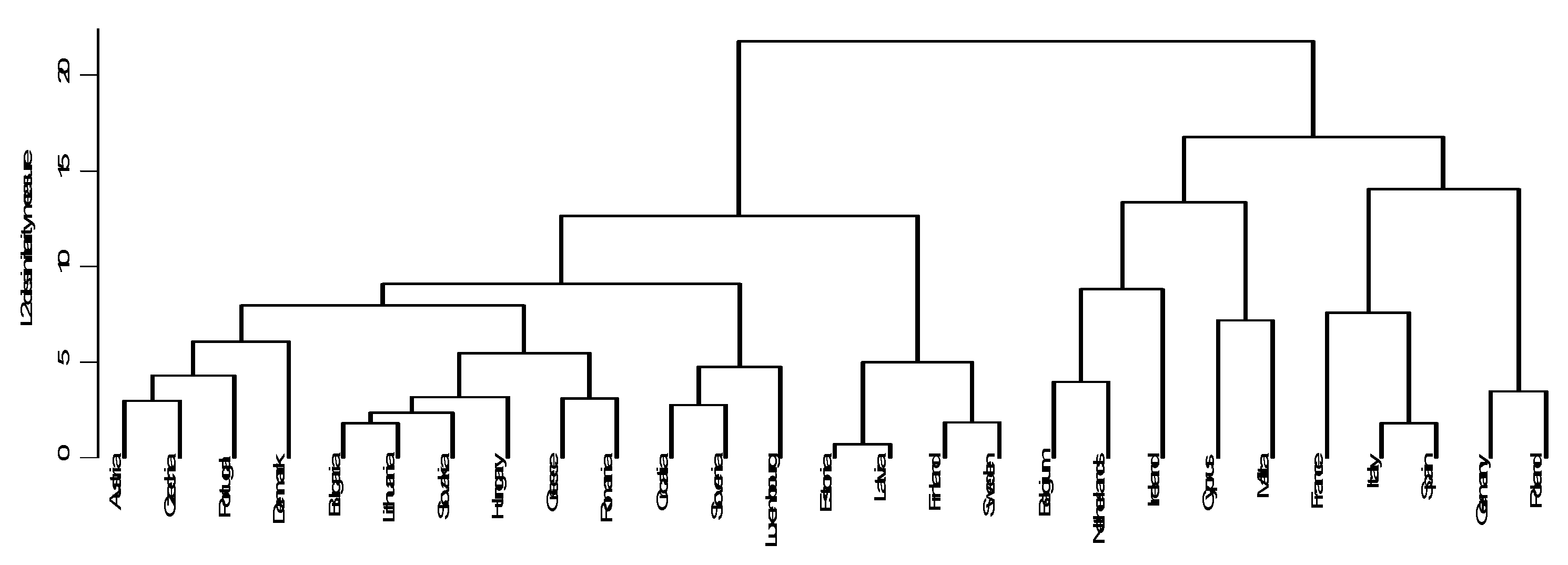
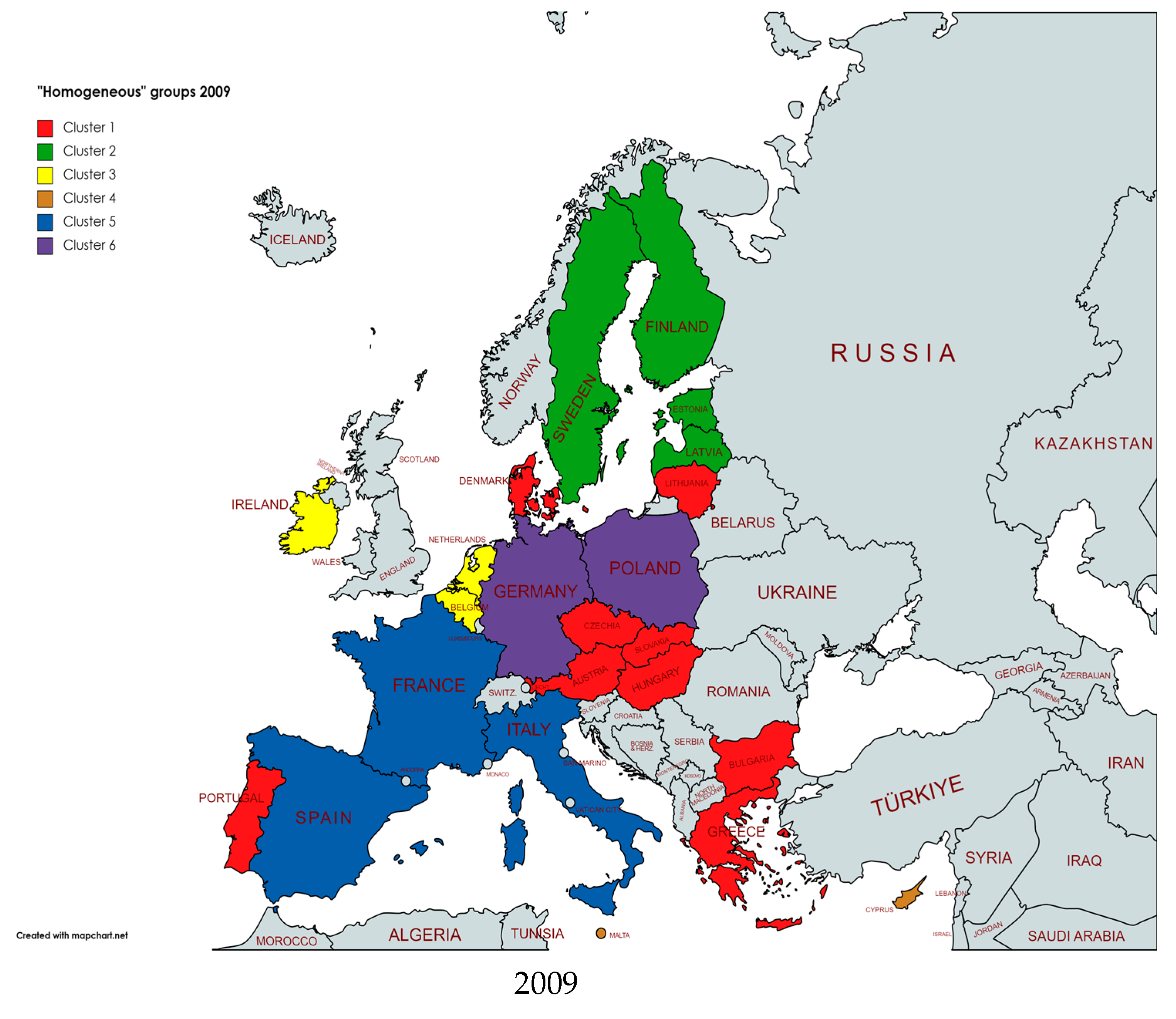
Furthermore, the statistical analysis carried out on the main PCs of the 2009 and 2019 agricultural systems allowed the 27 Member States to be grouped into 6 significant clusters or “homogeneous” groups.
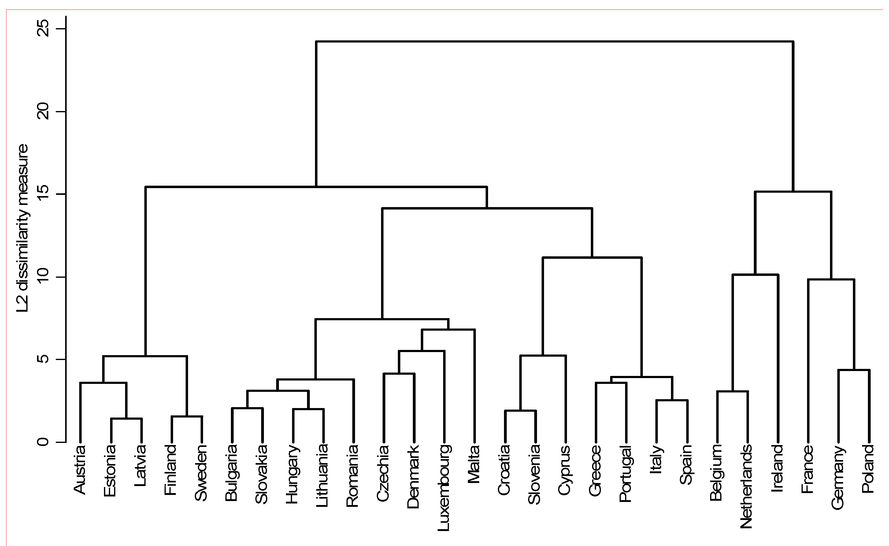
For 2009, the division into clusters (
Figure 2 and
Figure 3), using the complete linkage method, is as follows:
Cluster 1 includes 13 countries (which represent 48% of the total), located in northern and central Europe. The main characteristic of this first and largest group is the high reduction in the emission of CO2 from forestland. Slovenia and Slovakia show the highest reduction, −11,895.5 and −8863.15 kilotonnes, respectively.
Cluster 2 consists of four countries, showing a dynamic in the use of pollutants. On average, the countries of this group, especially Finland and Sweden, highlight a high emission of CCO2 from croplands. On average, the countries of this group, especially Finland and Sweden, highlight a high emission of CCO2 from croplands.
Cluster 3 includes the countries that show the highest average use per area of cropland (kg/ha) of all pollutants and pesticides, especially the use of K2O. On average, the countries of this group, in particular Ireland, show a high share of land under permanent crops in relation to the total land area. Furthermore, the countries of this group show a high incidence of cattle units per agricultural land area (LSU/ha). As is well documented, the latter are the main source of CH4 emissions compared to other ruminants, such as sheep.
In Cluster 4, there are only two countries: Cyprus and Malta. For this group, almost all the variables considered have below EU average values. Thus, this group is characterized by an absence of emissions from crops and from grasslands.
Cluster 5 groups together three countries (France, Italy and Spain) and is characterized, with respect to other clusters, by the low use of pollutants, especially N, and for high emissions of manure, measured in kilotonnes.
Cluster 6 consists, like Group 4, of only two countries (Germany and Poland) that, on average, in respect to the other five clusters, highlight the lowest use of pesticides per area of cropland (236 kg for ha).
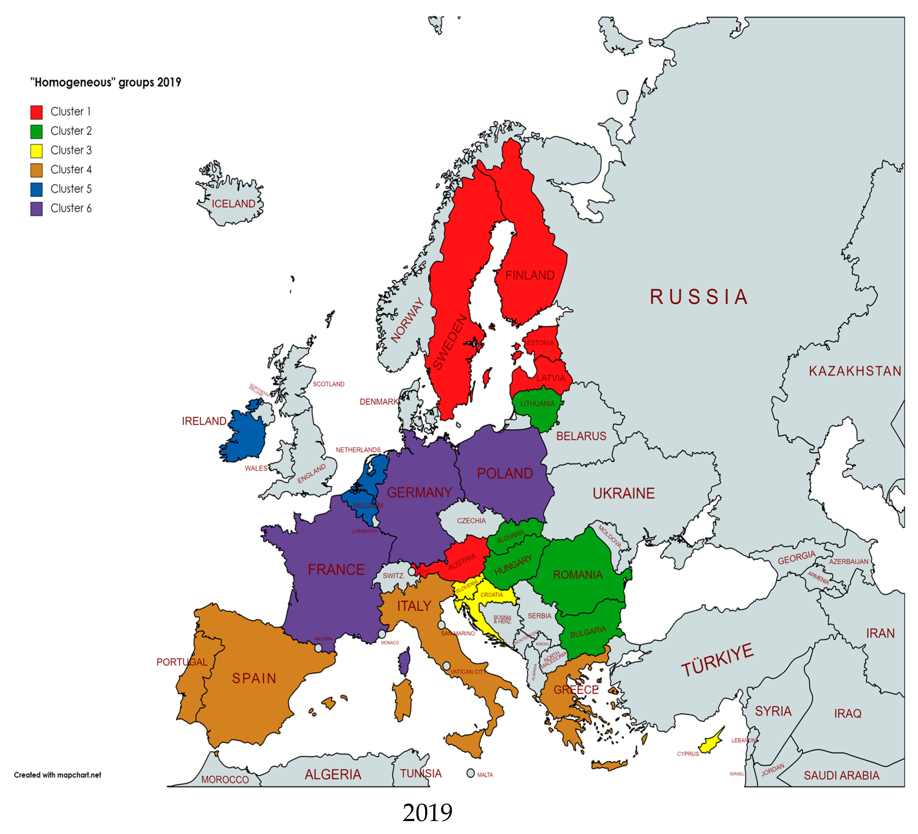
The 2019 cluster analysis conducted on the main PCs also generated six “homogeneous” groups of countries (
Figure 3 and
Figure 4).
Cluster 1 includes five countries (Austria, Estonia, Finland, Latvia, and Sweden) that, on average, show the highest incidence of forest land in the land area (60% vs. circa 35% of the global mean) and the highest incidence of organic agriculture in an agricultural area (19.27% vs. 9.33 of the global mean).
Cluster 2 is the largest, with nine countries (33% of the total EU countries), that, on average, present the highest share of agricultural land, arable land, and cropland in relation to the total land area.
Cluster 3 includes three countries, and is characterized by a high incidence of both the use of nutrient phosphate per area of cropland (38.48 kg/ha vs. 21.85 of the global mean) and of naturally regenerating forest on forest land (91.26 vs. 63.32 of the global mean).
Cluster 4 contains four EU countries with the highest presence of land under permanent meadows and pastures in relation to the total land area (19.22% vs. 5.72 of the global mean). Furthermore, this area has the highest share of sheep in relation to the total livestock area, suggesting a transition of these countries towards an intensification of agricultural activities.
Cluster 5 includes three EU countries with a strong presence of intensive agricultural activities, especially in terms of the use of both N per area of cropland (kg/ha) and pesticides, and in the presence of cattle.
Cluster 6, like Cluster 5, has only three EU countries that are the most responsible for crop, grassland, and livestock emissions with respect to the other five groups.
3.3. Discussion of Results from Non-Parametric Convergence Analysis
The values assumed by the indices
α and
β (
Table 5) can be accepted as weak convergence (or divergence) indices, as this is a convergence/divergence process conditioned by country choice and agricultural system variables.
Table 5 also shows that the value of α 1 (α 1, 2019–α 1, 2009) decreased mainly for the following agricultural systems variables: the share of the arable land; for the kg of N used per area of cropland; and the naturally regenerating forest (NRF). The standard deviation values α 1, 2009 and α 1, 2019 show an increase in the dispersion of variables examined around the mean quadratic average values over time, with a tendency towards divergence among countries with a high percentage of arable and agricultural land and those characterized by high livestock intensity.
Conversely, the synthetic index β highlights a divergence process for most variables and for all countries but shows a greater tendency for eco-friendlier countries to move away from those that continue to have IFSs. In accordance with Giller et al. [
58], this process was also influenced by the need to reform “conventional” agriculture according to the principles of agroecology, organic agriculture, and (increasingly) regenerative agriculture.
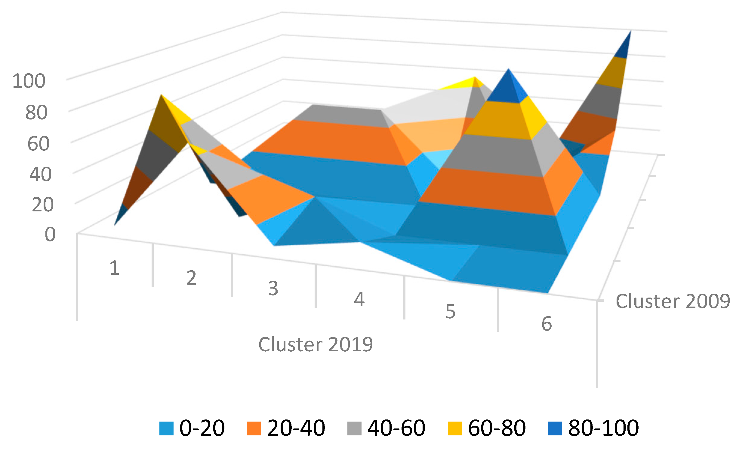
Table 6 shows that most EU countries have not remained in the same groups. The percentage value that appears in the transition Markoviana matrix [
43] indicates the number of times a country that belonged to one of the initial groups in 2009 passed into the same group in 2019. The most obvious element with reference to the transition matrix (TM) is that many countries have moved from their original group. Indeed, in the first row of the TM, for example, only Austria (A) of the twelve EU countries that in 2009 were in Cluster 1 remained in the same cluster in 2019. Seventy-five percent (Bulgaria, Czech Republic, Denmark, Hungary, Lithuania, Luxemburg, Malta, Romania and Slovakia) passed to Cluster 2, and just two countries (Croatia and Greece) passed to Clusters 3 and 4, respectively. The second line shows that 80% (Estonia, Finland, Latvia and Sweden) of the five countries that in 2009 belonged to Group 2 migrated to Group 1; the remaining 20% (Slovenia) moved to Group 3. The figures in the third line indicate that the three countries (Belgium, Ireland and the Netherlands) that belonged to Group 1 in 2009 had moved to Group 3 by 2019. The fourth line shows that the two countries (Cyprus and Malta) that in 2009 were in Cluster 4 passed to Clusters 2 and 3, respectively. The fifth line shows that the three countries (France, Italy and Spain) that belonged in 2009 to Group 5 had moved to Group 4 (Italy and Spain) and 6 (France), respectively. Lastly, the sixth line shows that the two countries (Germany and Poland) that belonged to Group 6 in 2009 had remained in Group 6 by 2019. A process of divergence has therefore occurred. The TM allowed a three-dimensional graph to be drawn (
Figure 5).
The main conclusion from this part of the analysis, in line with the literature on growth and convergence [
59], confirms that, from 2009 to 2019, the β convergence hypothesis interested, above all, countries with initially high levels of IFSs (Belgium, Hungary, Luxemburg, Romania). These countries tend to differ over time from those that have recently adopted an intensive agricultural system with high GHG emissions (Estonia, Finland, Latvia, and Sweden). These results can be verified by simply observing the data on the trends in EU countries’ FSs (
Table 3). It is possible, in accordance with Schmalensee et al. [
60], that high-income countries have continued to reduce their CHG emissions over the 2009–2019 period. Conversely, others in the same area, such as Sweden and Finland, have increased these emissions in the same period. Moreover, some Eastern European countries, such as Bulgaria, Czechia, Hungary, Poland, and Slovakia, have reduced GHG emissions even more than the richest EU countries.


