Article

UAV Monitoring Topsoil Moisture in an Alpine Meadow on the Qinghai–Tibet Plateau

1
State Key Laboratory of Herbage Improvement and Grassland Agro-Ecosystems, Key Laboratory of Grassland Livestock Industry Innovation Ministry of Agriculture, Northwest Degraded Grassland Ecological Restoration and Utilization Engineering Technology Research Center, National Forestry and Grassland Administration, College of Pastoral Agriculture Science and Technology, Lanzhou University, Lanzhou 730020, China
2
School of Geographical Sciences, Nantong University, Nantong 226007, China
*
Author to whom correspondence should be addressed.
Agronomy 2023, 13(9), 2193; https://doi.org/10.3390/agronomy13092193
Submission received: 26 July 2023 / Revised: 15 August 2023 / Accepted: 19 August 2023 / Published: 22 August 2023
(This article belongs to the Section Grassland and Pasture Science)

Abstract

:
Soil moisture is one of the most critical soil components for sustained plant growth and grassland management. Unmanned aerial vehicles (UAVs) are gradually replacing manual labor in various aspects of grassland management. However, their potential for monitoring soil moisture in grasslands remains largely unexplored. High vegetation coverage and frequent rainfall in the Tibetan Plateau pose a challenge for personnel working in alpine meadows. To explore the potential of UAV technology for soil moisture detection in these areas, we conducted a rainfall reduction experiment in Maqu County, China to understand the relationships among soil moisture, vegetation coverage, and visible-light images captured using UAVs. The findings indicated a significant correlation between topsoil moisture and the brightness values in visible-light images acquired by UAVs (p < 0.0001). These results demonstrated that visible-light brightness, vegetation coverage, rainfall reduction, and aboveground biomass can be utilized for estimating the topsoil moisture using these images (y = −0.2676 × Brightness + 0.2808 × Vegetation coverage −0.1862 × Rainfall reduction + 0.1357 × Aboveground biomass + 37.77). The model validation worked well (E = 0.8291, RS = −3.58%, RMA = 10.38%, RMSE = 3.5878, Pearson’s r = 0.9631, PSI = 0.0125). This study further addresses the problem of topsoil moisture measurement in flat areas of mesoscale moist alpine meadows and is expected to facilitate the widespread adoption of UAV use in grassland ecology research.

1. Introduction

The global grassland area is 5.25 billion hectares, which accounts for 40.5% of the global land area [1]. Globally, the relationship between precipitation and temperature determines the distribution, structure, and function of grasslands [2]. Most grasslands are located in harsh and remote areas that are characterized by severe cold or high temperatures, high altitudes, drought, or soil salinization [3]. Soil moisture (SM) is one of the key soil properties that plays an important role in maintaining grassland plant classification, productivity, biodiversity, structure, and function [4]. The SM of grasslands is mainly dependent on precipitation at large spatial scales and is influenced by human activities, including grazing, irrigation, mowing, and cultivation [5]. The interaction between vegetation and water is one of the important ecological processes in the ecosystem [6]. The SM directly affects grassland vegetation coverage [7]. As the main driving factor of plant diversity and biomass change, water affects plant growth [8]. At present, the methods for SM measurement, such as the traditional drying method, specific gravity method, and time domain reflection method (TDR), are simple to operate, but require manpower and other material resources [9]. Moreover, the drying method and the specific gravity method destroy the soil layer, which is not conducive to the sustainable development of the grassland ecosystem [10,11]. These protocols are suitable for the determination of the SM at the point scale [11,12,13]. There are several limitations in the determination of the SM such as in harsh climates, when considering the presence of aggressive wild animals, and when examining large- and medium-sized spatial-scale grasslands [14].
Satellite remote sensing technology provides a new method for SM measurement, with the advantages of low cost, high efficiency, and high spatial and temporal resolution [15,16]. However, the remote sensing image has only three visible light bands of R (red band), G (green band), and B (blue band), and the quantitative analysis has the limitation of collinearity [17,18]. Therefore, the HSB (hue, saturation, and brightness) transform must be performed on the R, G, and B visible-light images, and the correlation between the three channels of the HSB must be significantly lower than the correlation between the three bands of R, G, and B, which can better reflect the vegetation information [19]. The RGB images and artificial neural networks estimated the soil moisture in the different tropical regions of Brazil in 2015 [20]. Different linear models using the RGB values, the HSV (hue, saturation, and value) values, and the digital numbers of a panchromatic image were used to estimate six types of SM in the Federal University database in 2016 [21]. The intensity index, the TGI index, and the ExGreen index of aerial visible images (red, green, and blue bands) could be carried out to determine trends of soil moisture in agricultural land, where the TGI index has a higher coefficient of determination [22]. The visible-light technology of a UAV was used to establish the estimation method of species composition, and the visible light (B) of a UAV was used to establish the monitoring method of multiscale plant species diversity (PSD) of a large alpine grassland community [23,24]. In the field of UAV visible-light image processing, the average pixel brightness value calculated by the computer is usually used to reflect the brightness of the image [25]. The value of the parameter (brightness) is the pixel value of the RGB color image given by the remote sensing processing software [26,27]. Brightness is also closely related to plant greenness, vegetation coverage, and plant growth [28]. Plant brightness also reflects the changes in the plant and soil water content over a certain period of time [29]. Low-altitude multirotor unmanned aerial vehicles (UAVs) have the characteristics of small size, flexible flight, and short take-off distance. They have been widely used to study vegetation coverage, biomass prediction, land patches, mounds, vegetation species diversity estimation and livestock feeding behavior through the tracking of various grassland types [30]. We assumed that the visible-light brightness of UAV images combined with related indicators can be used for the SM prediction of different grassland types at different spatial and temporal scales.
The Qinghai–Tibet Plateau (QTP) is the largest and most continuous grazing land in the world, with alpine meadows being the main vegetation type [31]. The soil and vegetation are sensitive to water due to high altitude and a large variability in precipitation [32]. Based on the UAV visible-light brightness technology, we established a monitoring method for measuring the soil moisture of the typical steppe through precipitation addition to establish a soil moisture gradient in the areas with an annual precipitation < 400 mm in northern China [33]. However, it has not been verified in alpine meadows with an annual precipitation > 550 mm. To test this hypothesis, we conducted a field study in the QTP. A prediction model between the SM and visible-light reflectance was obtained by using the visible-light brightness of a UAV as the key factor for soil moisture prediction. It provides a new method for the ecological and environmental monitoring of the QTP and a method for rapid soil moisture determination for precision agriculture and formula fertilization. The research aims were as follows: (1) to evaluate the direct relationship between the vegetation coverage and UAV visible-light brightness. (2) to establish a prediction model between the SM and visible light under different water gradients, and (3) to calibrate and verify model parameters at different time scales.

2. Materials and Methods
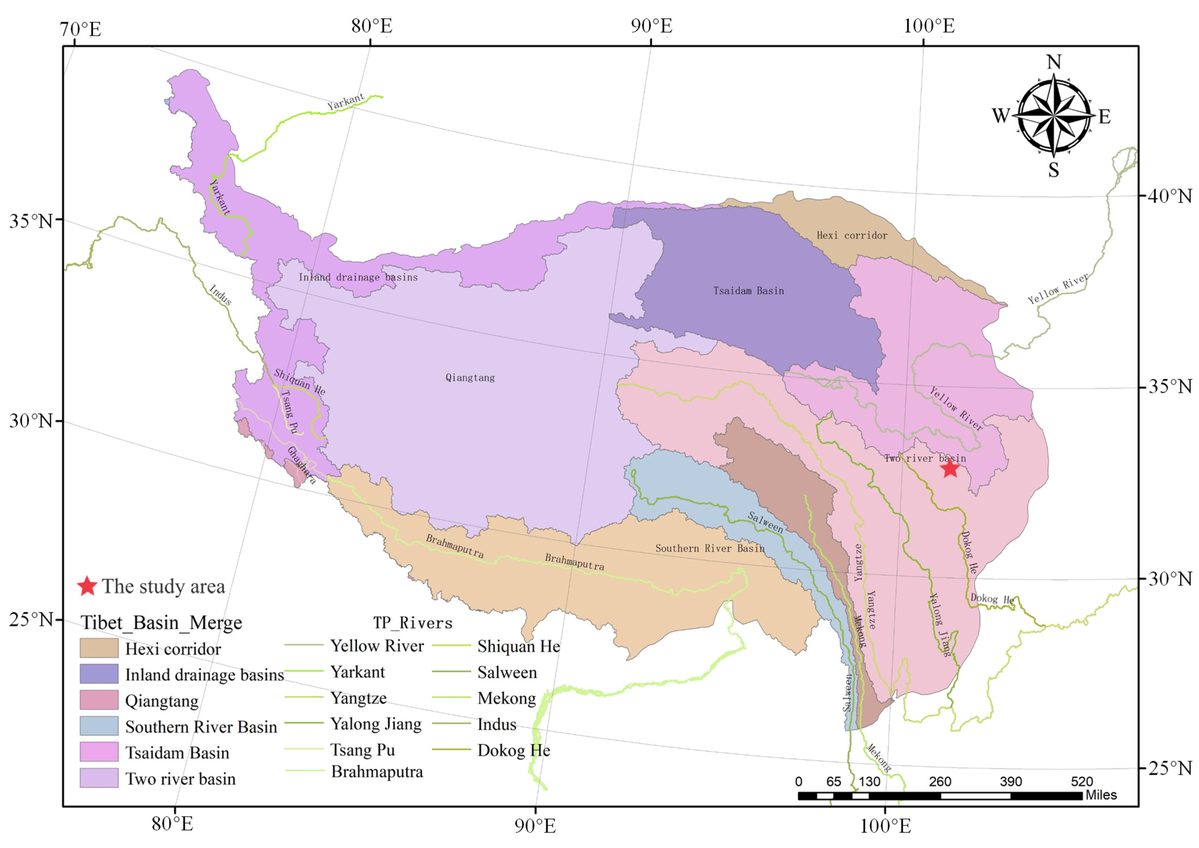
2.1. Study Area

The study was conducted at Maqu Grassland Agricultural Research Station of Lanzhou University (33°41′ N, 101°51′ E; elevation 3455 m), Maqu County, Gansu Province, China, located in the northeast of the Qinghai–Tibet Plateau. Grazing experiment of Tibetan sheep and yaks has been conducted since 2010 (Figure 1). It has a plateau continental climate. From 2019 to 2020, the mean annual temperature was 2.8 °C, with a maximum of 11.7 °C in the middle of August. The annual precipitation was 724.1 mm, which was mainly concentrated from June to August, which accounted for 59% of the annual total precipitation (Figure 2). Annual sunshine was approximately 2580 h, there was an annual frost period of approximately 270 days, and there was no absolute frost-free period. The grassland is classified as an alpine meadow, and soil is classified as subalpine meadow soil [34]. The main plant species are Elymus nutans, Koeleria cristata, Kobresia graminifolia, Kobresia capillifolia, and Kobresia pygmaea [35,36].

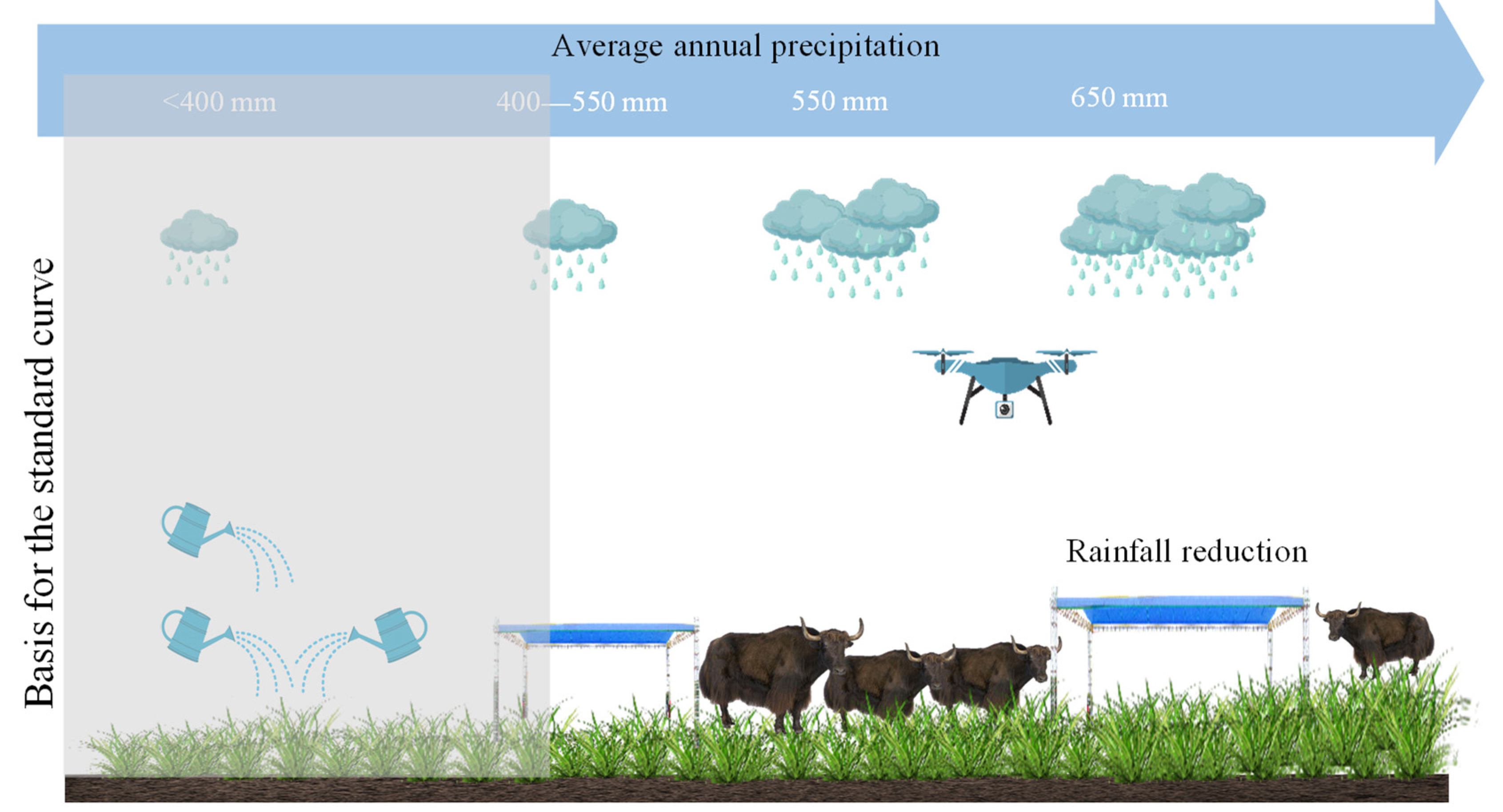
2.2. Experimental Design

2.2.1. Sample Plot Setup

Since 2019, grazing has been carried out in the four-season rotational grazing area of Maqu Grassland Agricultural Research Station of Lanzhou University in Gansu Province from June to August. The grazing area in each season was 1.5 ha, and 80 yaks with similar body conditions graze evenly for 21 days from 06:30 to 16:30 in all seasons, free grazing outside the four-seasonal grazing area.
To fit the curve of annual precipitation due to the high variability, the theoretical maximum SM was estimated by different methods using natural evapotranspiration to create a moisture gradient. In the areas with low annual precipitation (<400 mm), irrigation was used to establish a gradient [33]. The QTP has a large annual rainfall (>550 mm), and the phenomenon of night rain is a typical climate characteristic of the QTP, with an average night rain rate of 80% [8]. The total precipitation from June to August accounts for about 59% of the annual precipitation, which is the most sensitive period of vegetation to precipitation. Therefore, we chose to employ rainfall reduction at night and open sites during the day from June to August, which does not affect plant photosynthesis and growth (Figure 3). Ten sampling sites (2 m × 2 m) were selected from the representative free-grazing areas with flat terrain and uniform vegetation; five were used as rainfall reduction samples and five as control samples. The rainfall reduction samples were fixed and the control samples were not fixed. Transparent plastic sheets were placed on top of the sheltered wooden frames with a base area of 3 m × 3 m and a height of 1.5 m to block rainfall during precipitation events and were removed after the rainfall stopped. We estimated the vegetation coverage in the sample box of 0.25 m2, counted the number of plant species, put them into envelope bags, and weighed their fresh weight, followed by blanching at 105 °C for 30 min, drying at 65 °C for 72 h, and determination of the dry weight. Species richness was obtained as the sum of all species present in the plots. In the case of the rainfall reduction samples, the separation of the deep soil from the topsoil moisture was the same as that of the irrigated samples. The soil moisture content was measured every 2–3 days at midday in the local area owing to the slow change in soil moisture content. Since vegetation is more dependent on the soil moisture from 0 to 10 cm, a TZS-5X-G soil moisture tester was used to measure the soil moisture from 0 to 10 cm. Two 0–10 cm soil samples were collected using a 50 mm diameter stainless steel soil auger and transported back to the laboratory in self-sealing bags. The soil samples from each plot were mixed, impurities such as plant tissues and apoplasts were removed with a 2 mm sieve, samples were dried indoors in the shade, and soil moisture was determined by the drying method.

2.2.2. Research Route

A rainfall reduction test was conducted in the free-grazing area to explore the use of UAV technology to assess the soil moisture content of grasslands. Results were then used to develop a conceptual model and an actual estimation model, followed by a rotational grazing test performed in the enclosed rotational grazing area to verify the practicality of the estimation model (Figure 4).

2.3. Acquisition of UAV Image Data

2.3.1. Set UAV Parameters

The brightness value of the image is influenced by light intensity, UAV flight speed, and visible-light camera parameters (i.e., model, lens angle, ISO, aperture, and shutter speed). Among these factors, the UAV flight speed and visible-light camera parameters are controllable, and, therefore, the most suitable settings were selected for these parameters (Table 1).

2.3.2. Image Acquisition

The light intensity is an uncontrollable influence factor affected by both the solar altitude angle and atmospheric transparency. To unify the solar altitude angle among aerial photography dates, the local midday period (12:00–13:00) was selected for photography, and the errors caused by the differences in atmospheric transparency and midday solar altitude angle between seasons were subsequently corrected. Moreover, to match the soil moisture content, aerial photography was synchronized with the determination of soil moisture content from 0–10 cm, and aerial photography was postponed in the case of midday rainy weather.
The automatic flight of the UAV (DJI Mavic Air 2) was made every 2–3 days to photograph the rainfall reduction and the control samples during the rainfall reduction test in the free-grazing land. The flight mode settings were an airspeed of 3 m/s, altitude of 3 m, vertical image capture, and coverage of more than 2 × 2 m grasslands in a single image. The plant visible-light images collected by the UAV only analyzed the images within sample plots of 0.25 m2. For the validation sample of the four-season rotational grazing land, aerial photography from the UAV was conducted in the same modes and at the same time as used for the soil moisture content measurements.

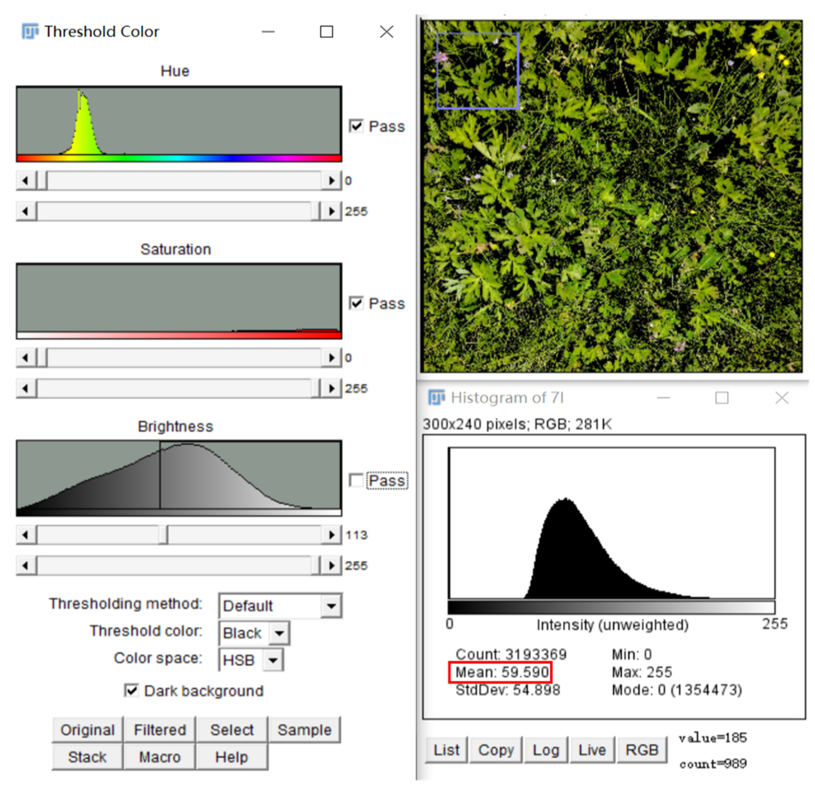
2.3.3. Image Acquisition of Vegetation Coverage

ImageJ software was used to divide a UAV visible image into vegetation coverage and soil coverage based on the appropriate hue, saturation, and brightness (HSB) settings. The HSB settinga used in this study are shown in Figure 5: (a) Specifically, the “threshold color” option of ImageJ was selected, and the HSB was set to the optimal values to select the vegetation coverage portion. (b) The vegetation coverage portion was adjusted. (c) The final selected portion was preserved, and the vegetation coverage area was output by the software.

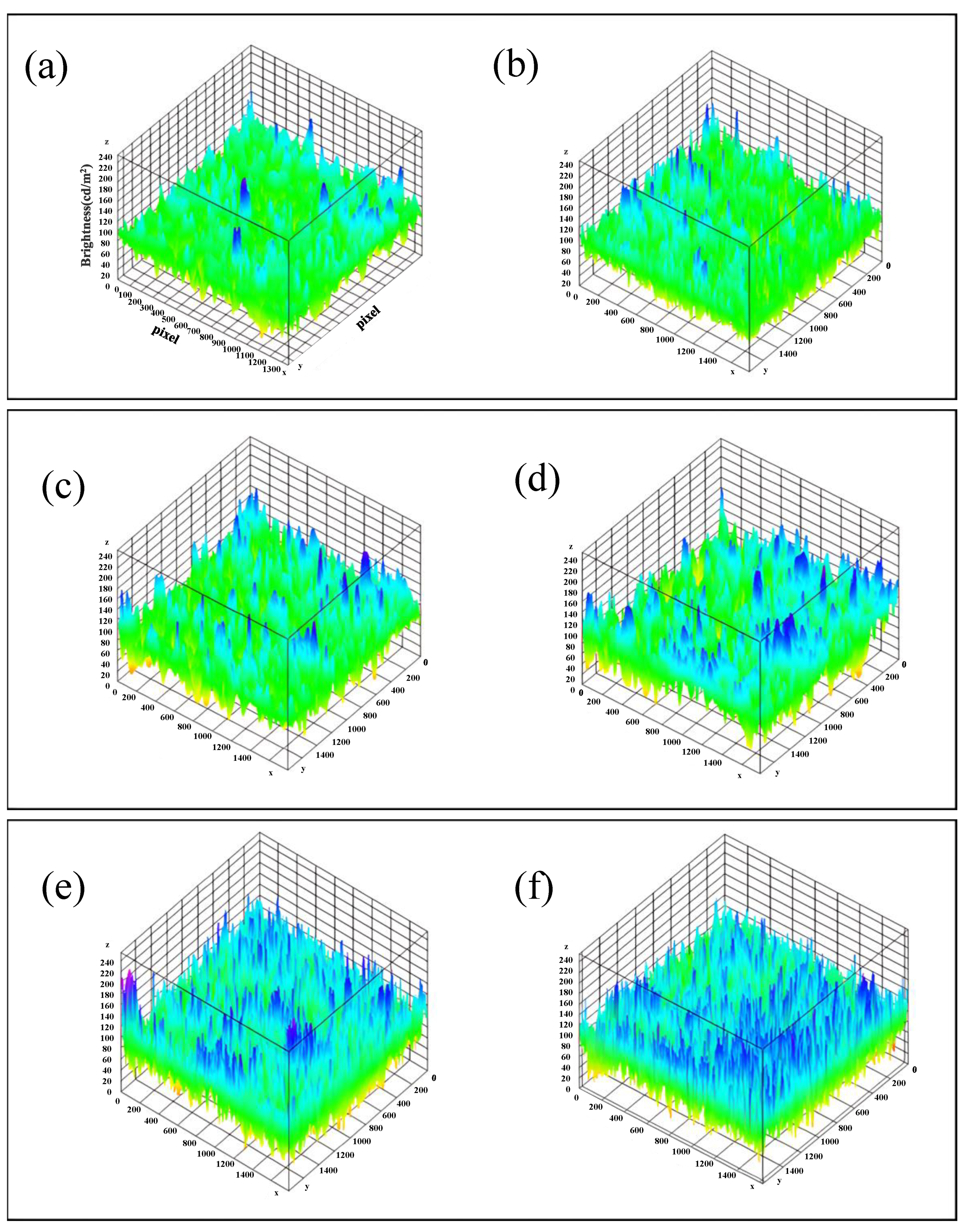
2.3.4. Acquisition of Brightness Value of Visible Light Image

Since the visible-light images captured by UAVs were RGB color images, the “pixel-averaged brightness value” was introduced (hereinafter referred as the “brightness value”). The value of this parameter is the pixel value assigned to the RGB (The RGB range is 0 to 255) color image by the ImageJ, thus reflecting the difference in brightness of the color image obtained through the formula 0.30 × R + 0.59 × G + 0.11 × B, where R, G, and B represent the red, green, and blue channels of the color image, respectively [26,27]. The brightness value of RGB color images reflect the surface reflection of visible electromagnetic radiation to some extent [37]. The luminance value of visible-light images was influenced by the light intensity, and since the study area on the QTP has typically cloudy and rainy weather, and the surface was almost completely covered by vegetation, the change in soil moisture content can only be reflected by the vegetation, which will produce color changes due to the influence on soil moisture. Therefore, for the visible-light images of the vegetation, we first selected the vegetation portion of the image using the color threshold function of ImageJ software and then adjusted the color threshold according to the unified HSB standard, thereby obtaining the average brightness value from the histogram function (Figure 6).

2.3.5. Influence Factor Control and Error Calibration of Visible-Light Images

The variation in the greenness, as a research indicator of UAV visible-light images, belongs to the variation of hue, which is the primary feature of color and is the most accurate variation for distinguishing different colors [38]. The greenness in the study area depends on the increase or decrease of the green portion of the image and is affected by the solar altitude angle; a higher solar altitude angle will result in more solar radiation per unit area. As the temperature changes, part of the light will produce color changes, thereby affecting the hue of visible-light images [39]. To prevent the brightness values of visible-light images from potentially interfering with the hue, a local date with low midday cloudiness was selected for UAV visible-light image capture so that the brightness values remained at similar levels. The camera lens of the DJI Mavic Air 2 UAV has an automatic white balance setting, which corrects the hue difference caused by the solar altitude angle (color temperature).

2.4. Statistical Analysis

Microsoft Office Excel 2019 was used for data entry and organization, and SPSS was used for statistical analysis. Origin (OriginLab, Northampton, MA, USA) software was used for constructing charts. ImageJ was utilized to draw the histograms, grayscale images, and three-dimensional (3D) surface maps of the UAV visible-light images. Structural equation model analysis was performed using IBM SPSS Amos 21.0.
The brightness data from the visible-light images captured by the UAV, which contained areas of different 0–10 cm soil moisture contents, were analyzed. From left to right in June, the observed 0–10 cm soil moisture values were 43.52%, 39.04%, and 36.97%, respectively (Figure 7a).
The UAV visible-light images were divided into three parts based on soil moisture, which were then input into ImageJ for processing. First, the visible image was converted to an 8-bit grayscale image. A grayscale image has 256 brightness levels, with 0 at the darkest end of the scale and 255 at the brightest end. A spectral filter was added to the grayscale images via the “lookup table” mode in ImageJ to significantly stratify the brightness of the grayscale images. Thus, we roughly divided the grayscale image with 256 levels of brightness into seven colors: red, orange, yellow, green, cyan, blue, and violet (from dark to light). The luminance gradually increased from the left figure to the right figure (Figure 7b).
Second, to visually compare the brightness differences, a 3D surface map was used to convert the brightness-to-height information and to translate the concept of dark-to-light to measures of low-to-high (Figure 7c).
Finally, histograms were output. In these histograms, the “mean” refers to brightness. As shown in Figure 7d, 43.52%, 39.04%, and 36.97% of the soil moisture from 0 to 10 cm correspond to luminance values of 88.396 cd/m2, 93.497 cd/m2, and 95.503 cd/m2, respectively. The difference in soil moisture from 0–10 cm is thus reflected in the brightness of the visible-light images of the UAV (Figure 7d).

2.5. Model Establishment for UAV Technology Assessment of the 0–10 cm Soil Moisture in an Alpine Meadow

In alpine meadows on the QTP, the conceptual model for UAV assessment of the 0–10 cm soil moisture in grasslands relies on the surface hue condition (which depends on greenness changes) during the process of feedback to vegetation, as revealed by the feature factor of UAV visible-light images. In this study, vegetation changes in alpine meadows on the QTP with different levels of 0–10 cm soil moisture were detected by the UAV visible-light camera.

2.6. Validation of the Practicality of the Estimation Model

The coefficient of determination (R2) and model efficiency (E) were used to evaluate the predictive ability of the 0–10 cm soil moisture estimation model. The absolute value of the total relative error (RS), average relative error (RMA), root mean square error (RMSE), and Pearson product–moment correlation coefficient (r) was used to verify the fit of the measured and estimated values from the validation sample analysis [40]. In general, better model accuracy is demonstrated the closer R2 and E are to 1, the closer RMSE is to 0, with a Pearson’s r tending to 1 or −1, with the absolute value of RS < 20%, with the absolute value of RMA < 30%, and with a PSI < 0.1, which meets the accuracy requirement. The calculation formulas are as follows:
E = 1 i = 1 n M i S i 2 i = 1 n M i M ¯ 2
R S = M i S i S i × 100 %
R M A = 1 n × i = 1 n M i S i S i × 100 %
R M S E = i = 1 n M i S i 2 n
P e a r s o n s   r = i = 1 n M i M ¯ S i S ¯ Σ = 1 n M i M ¯ 2 Σ = 1 n S i S ¯ 2
P S I = i = 1 n ( ( A c t u a l   p r o p o r t i o n E x p e c t e d   p r o p o r t i o n )   l n A c t u a l   p r o p o r t i o n E x p e c t e d   p r o p o r t i o n )
where Mi is the measured value of the sample, Si is the estimated value of the sample, and n is the number of validation samples; M ¯ is the average of M. S ¯ is the average of S.

3. Results

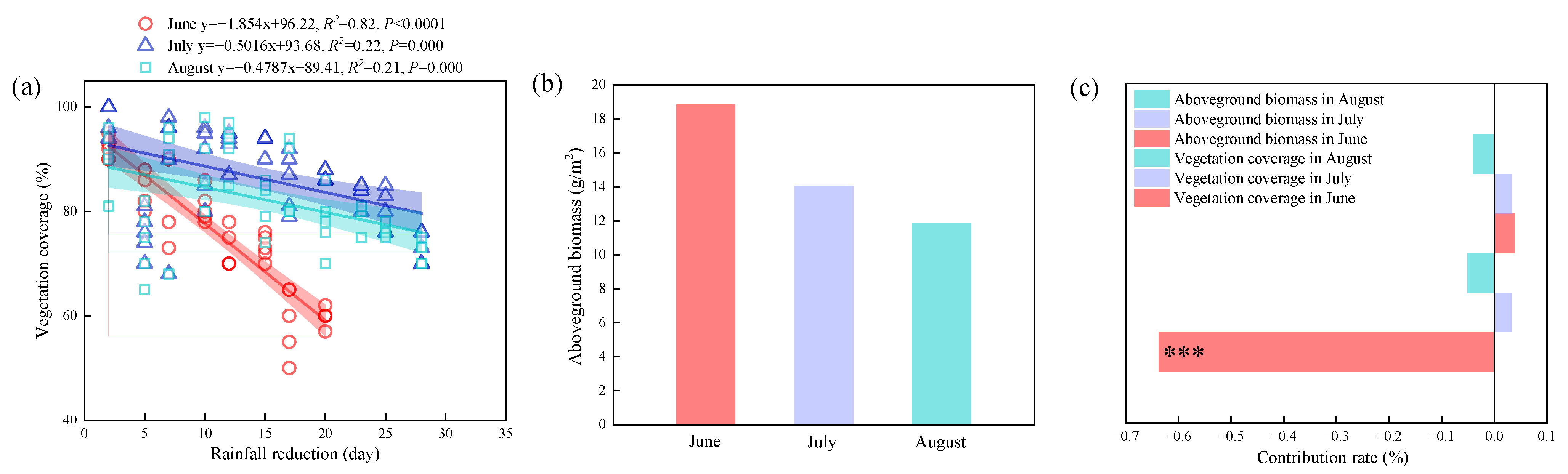
3.1. Effects of Rainfall Reduction on Vegetation Coverage and Aboveground Biomass

Vegetation coverage was negatively correlated with the duration of night rainfall reduction in June, July, and August (p < 0.001, Figure 8a). The aboveground biomass gradually decreased with the increase in rainfall reduction (Figure 8b). The contribution rate of the vegetation coverage in June to the rainfall reduction was the largest (Figure 8c).

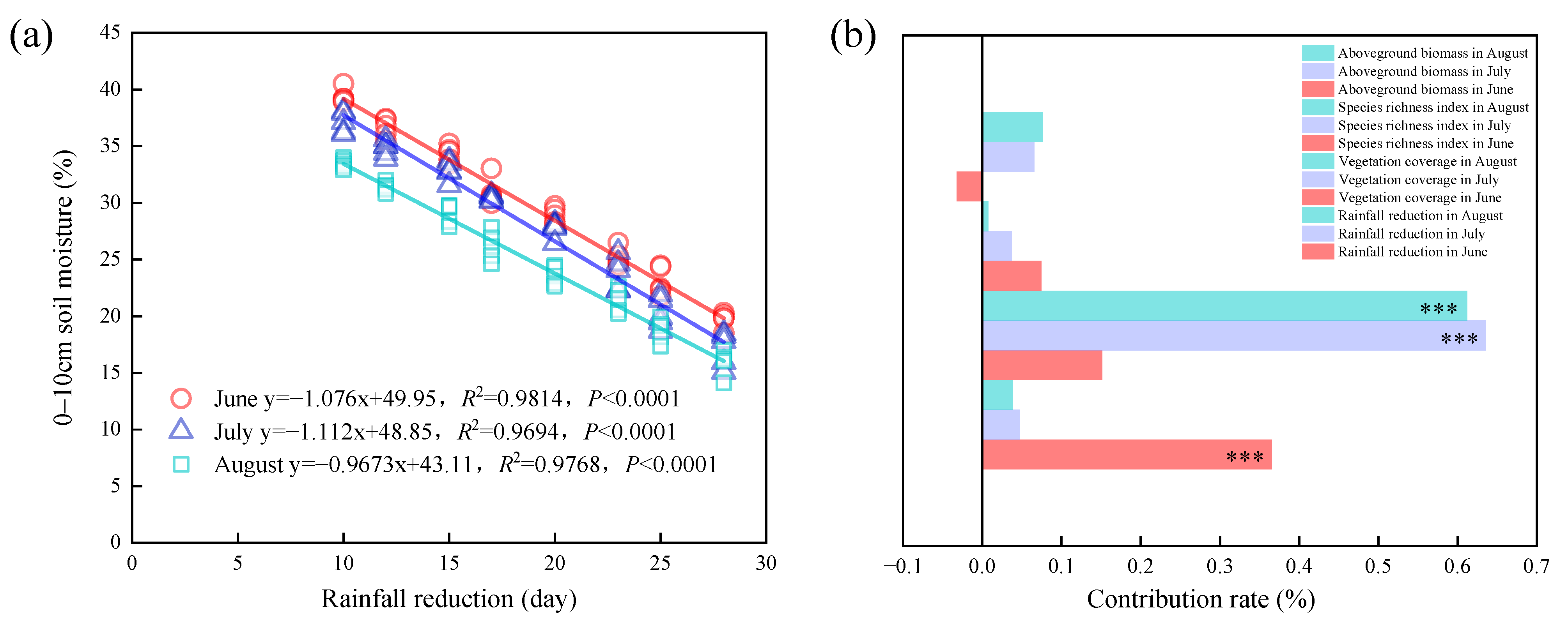
3.2. Effect of Rainfall Reduction on Topsoil Moisture

Night rainfall reduction was negatively correlated with topsoil moisture in different months (p < 0.0001, Figure 9a). The contribution rate of the vegetation coverage to the soil moisture was the largest in July, followed by the vegetation coverage in August and the rainfall reduction in June, while the contribution rate of species richness to the soil moisture was the smallest in August (Figure 9b).

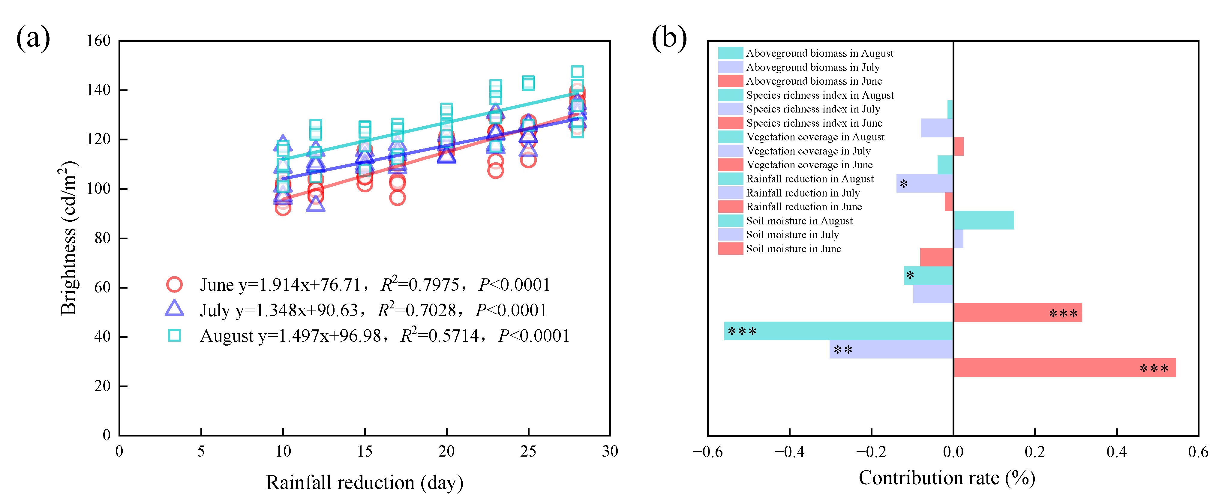
3.3. The Effect of Rainfall Reduction on Brightness

In alpine meadows of the QTP, the decline of the 0–10 cm soil moisture content accelerated the yellowing of the vegetation. The UAV visible-light images of a set of highland rainfall reduction samples were converted into a 3D surface plot using ImageJ software to compare the initial and later stages of the rainfall reduction. The images after rainfall reduction were darker in early June, early July, and early August and were brighter after the rainfall reduction (Figure 10).
The rainfall reduction was positively correlated with visible-light brightness values in different months (p < 0.0001, Figure 11a). The soil moisture in August contributed the most to the brightness, followed by the soil moisture and the night rainfall reduction in June (Figure 11b).

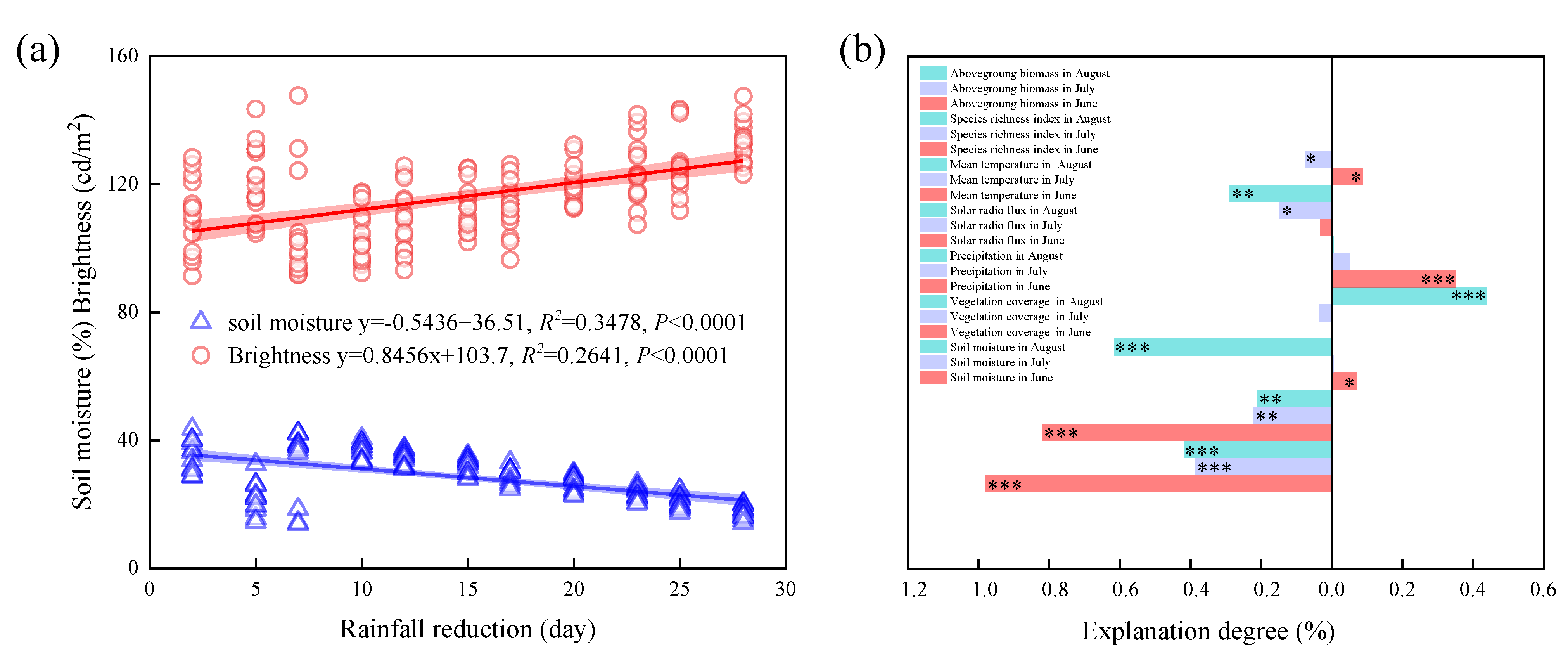
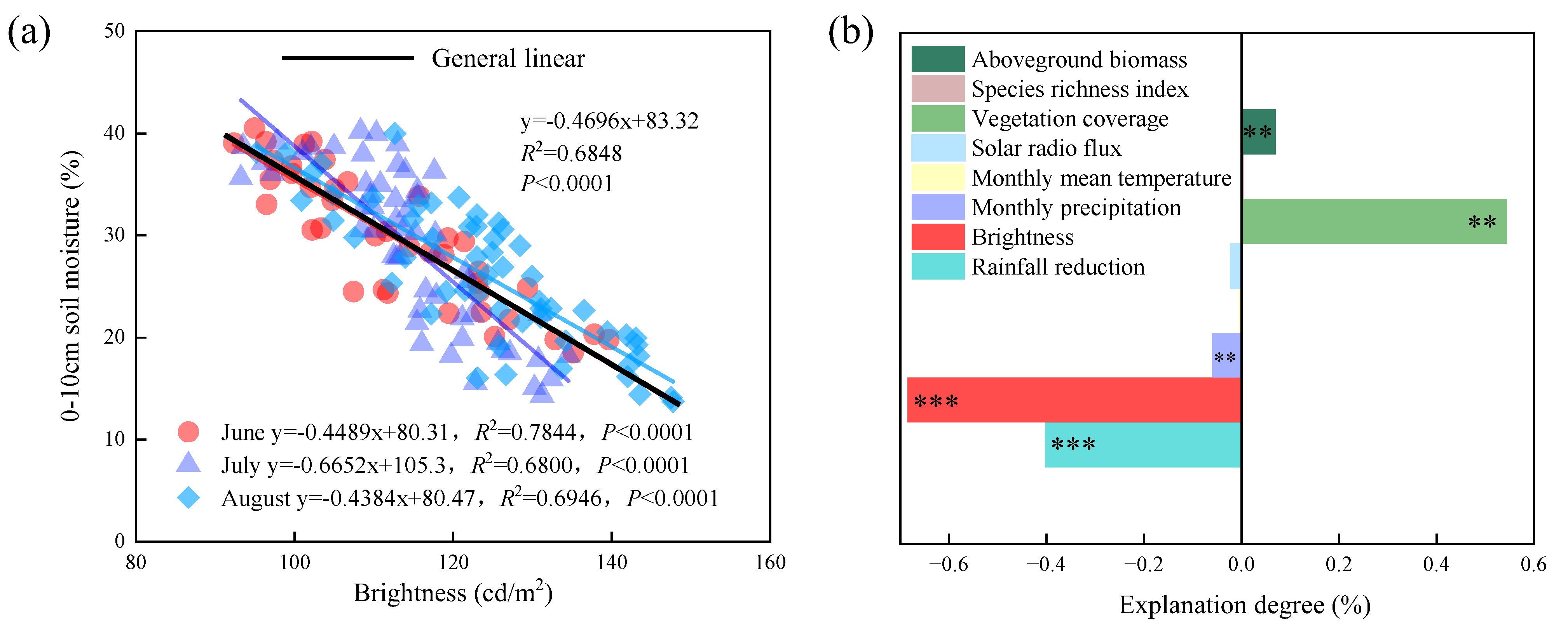
3.4. Effect of Rainfall Reduction on Soil Moisture-Brightness Relationship

The rainfall reduction was positively correlated with brightness and negatively correlated with soil moisture (p < 0.0001, Figure 12a). The explanation degree of the soil moisture to the nighttime rainfall reduction in June was the highest (98%), followed by the vegetation coverage in June (82%). The explanation degree of the aboveground biomass to the nighttime rainfall reduction in August was the smallest at only 0.2% (Figure 12b).

3.5. Model and Calibration of UAV Monitoring Soil Moisture

3.5.1. A General Linear Model for Predicting Soil Moisture According to Visible-Light Brightness

Using 2/3 of the data for June, July, and August as predictive models, the soil moisture and brightness were negatively correlated to obtain a general linear model y = −0.4696x + 83.82 (p < 0.0001, Figure 13a). The explanation degree of the brightness to the soil moisture was the largest, which was 68%, followed by the vegetation coverage and rainfall reduction, which were 54% and 41%, respectively (Figure 13b).

3.5.2. Calibration of General Linear Models

The multiple linear regression analysis showed that the brightness positively predicted surface soil moisture (p < 0.0001). The brightness and vegetation coverage were taken as the factors to explain the change in the SM, and the model effect was better (p < 0.0001). The best model predicted the soil moisture content according to the visible-light brightness, vegetation coverage, rainfall reduction, and aboveground biomass (y = −0.2676 × Brightness + 0.2808 × Vegetation coverage −0.1862 × Rainfall reduction + 0.1357 × Aboveground biomass + 37.77, R2 = 0.8610, p < 0.01, PSI = 0.0125) (Table 2).

3.5.3. Verification of Mixed Linear Model

The structural equation model (SEM) was constructed to analyze the accuracy of the soil moisture prediction model. The brightness, vegetation coverage, rainfall reduction, and aboveground biomass explained 55%, 34%, 19%, and 12% of the soil moisture, respectively. The brightness and vegetation coverage directly affected the SM, and the rainfall reduction had a significant indirect effect on the SM. The model works well (Figure 14).

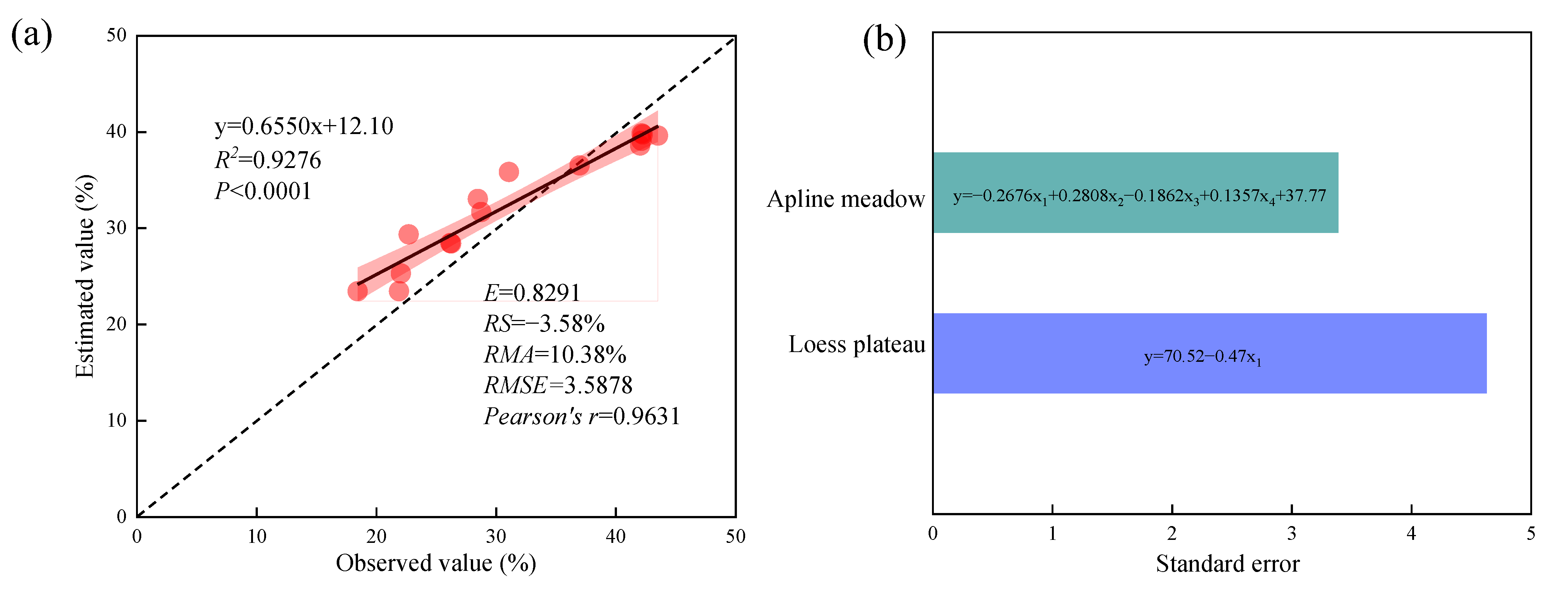
3.5.4. Model Application

The observed and estimated values of the remaining 1/3 of the 0–10 cm soil moisture data in June, July, and August were compared, and the correction coefficient was 0.9276. Among them, E = 0.8291, RS = −3.58%, RMA = 10.38%, RMSE = 3.5878, Pearson’s r = 0.9631, and PSI = 0.0125 through model validation. The multivariate linear model could predict the 0–10 cm soil moisture (y = −0.2676 × Brightness + 0.2808 × Vegetation coverage − 0.1862 × Rainfall reduction + 0.1357 × Aboveground biomass + 37.77). The standard error of the alpine meadow was small, the accuracy of prediction data was high, and it could be corrected (Figure 15).

4. Discussion

4.1. Effect of Rainfall Reduction on Vegetation-Soil Moisture and Visible Light Brightness

Soil moisture determines vegetation types and coverage to a great extent, and changes in the SM can be reflected by changes in the vegetation [41]. Vegetation will show color changes under the influence of soil moisture [42]. Changes in the soil moisture also directly affect the aboveground biomass [43]. In this experiment, there was a significant negative correlation between the rainfall reduction and the vegetation coverage in June, July, and August (Figure 8a). With the increase in rainfall reduction days, the aboveground biomass gradually decreased in June, July, and August (Figure 8b). The contribution rate values of the vegetation coverage to the rainfall reduction were the highest (Figure 8c). The coupling of temperature, precipitation, and soil properties leads to variation in the SM at different spatial and temporal scales [44]. This may be due to the influence of the temperature, ice, and snow thawing, thereby resulting in alpine meadow plants obtaining water to promote growth and development. Moreover, the plants absorb nutrients that change the SM levels [45,46]. There was a negative correlation between the SM and the rainfall reduction (p < 0.0001). The contribution rate of the rainfall reduction and the vegetation coverage to the SM was large (Figure 9). The main reason is that the precipitation intensity and intermittency of the rainfall reduction play an important role in the dynamics of vegetation cover and SM [47]. This might be due to the reason that the growth rate of the plants was higher at the beginning, which exceeded the supporting capacity of SM. The rapid growth of vegetation coverage may lead to insufficient SM content [48]. Previous research results showed that the infiltration rate of alpine grassland with high vegetation coverage was 125%, which was higher than that of grassland with low vegetation coverage [49]. Strong solar radio flux in high-altitude areas causes dramatic changes in the surface temperature [50]. Vegetation effectively reduces the near-surface radiation through photosynthesis and leaf shielding, thereby reducing the range of surface temperature changes, which is very important for soil–vegetation coupling [51,52].
In the field of UAV visible-light image processing, the “average pixel brightness value” calculated by the computer is used to reflect the brightness of the image, which is generally used for image color adjustment and photographic exposure correction [25]. In this study, we chose to reflect the change in the SM from the perspective of the visible-light brightness under unified correction. We used irrigation methods to establish a standard UAV visible-light brightness curve and a SM curve in arid areas (annual precipitation < 400 mm). The calibration coefficient reached 0.82, which accurately predicted the SM content of a typical steppe in the Loess Plateau [33]. The night rain phenomenon in the Tibetan Plateau is a typical climatic feature, with an average night rain rate of up to 80% [8]. Therefore, we used UAV visible-light technology in the alpine meadow to establish a series of standard curves for the visible-light brightness and SM through rainfall reduction at night experiments to build the adaptive SM prediction model for large-scale ecological areas. The results showed that the brightness increased significantly in the early and late stages of rainfall reduction. (Figure 10). The brightness value of the visible-light image is affected by many factors, such as rainfall reduction, vegetation coverage, species richness, and aboveground biomass (Figure 11). This may be due to the decrease in water content before and after rainfall reduction that accelerates the yellowing of plant leaves and increases the brightness value of the visible light [53]. There was a significant negative correlation between the SM and the brightness, and the brightness and vegetation coverage had the greatest contribution to the SM (p < 0.0001, Figure 13). Surface reflectance refers to the ratio between the surface reflection of the solar radiation and the total solar radiation [54]. In previous QTP studies, “surface reflectance” was used as a feature of visible light images. Water is necessary for plant growth, and the visible light layer of plants has a significant correlation with the reflection of the SM [55]. Surface reflectance usually strongly correlates with the SM, and each band has a corresponding surface reflectance [56]. The brightness of the rough surface band is higher than that of the smooth surface band. The reflectivity of the wet soil is lower than that of the dry soil [57,58]. The fluctuation of the SM makes the visible light reflectivity of the leaves change to a certain extent [59]. Water-deficient plants tend to collapse, thereby reducing the roughness of the horizontal plane of the visible light image to a certain extent and resulting in a significant increase in the brightness value [60]. When the soil moisture content suddenly increases, the plants usually grow well, thereby making the vegetation more upright and resulting in a rougher image captured by the drone from above. Compared with water-deficient plants, plants with sufficient water uptake exhibit a more erect shape, and the visible-light images before and after the shading of the 3D topographic maps become rougher [61,62]. Therefore, the greater the SM content, the less visible light that eventually reaches the UAV visible light camera, thereby resulting in a smaller average pixel brightness value of the visible-light image (Figure 13).

4.2. Applicability of Soil Moisture Model at Different Time Scales

In this study, the effect of brightness on the SM at 0–10 cm depths was assessed by the relationship between SM and the brightness of UAV visible images at different time scales (Figure 4). There are many reasons for the variation in brightness, such as rainfall reduction, vegetation cover, aboveground biomass, and species richness (Figure. 11). We first used the brightness of visible light to predict the SM and establish a general linear model (Figure 13). Secondly, the general linear model was corrected to obtain a multiple linear regression model with good results (Table 2). We performed an SEM validation test on the multiple linear regression model (Figure 14). The results showed that the combined effects of brightness, rainfall reduction, vegetation coverage, and aboveground biomass characterized the change in the surface SM, and the model effect was best with these variables (p < 0.01, R2 = 0.8610, PSI = 0.0125). Although we confirmed the superiority of the model in predicting the 0–10 cm depth SM, special attention was paid to the areas sampled in August, because summer grazing occurred from June–August and was largely over by late August. The overall SM was greater in June than in August (Figure 9a), and the overall brightness values were significantly greater in August than in June (Figure 11a). The SM dropped sharply in mid-July, and, according to the observations of local weather stations, high temperatures persisted during that period, thus indicating that the 0–10 cm depth of the SM was strongly influenced by the temperature. The maximum brightness values were in August, while the minimum values were in June (Figure 11a). This could be because the vegetation cover reached a relative maximum in June, while in August the vegetation started to turn yellow, and the cover started to decrease, thereby affecting the brightness values. This could also be due to livestock feeding and trampling reducing the cover of the edible pasture, thus increasing evaporation of the SM as the ground temperature rose, increasing soil compaction, and reducing water infiltration [63,64]. Thus, grazing intensity may significantly affect the SM content in 0–10 cm soil profile. Due to frequent livestock feeding, the free-grazing land was trampled to varying degrees, and the overall growth was lower than that of the seasonally grazed land [65,66]. As a result, the overall predicted values were skewed toward the upper left corner of the curve; i.e., the predicted values were generally higher than the measured values (Figure 15).

5. Conclusions

UAVs using visible-light technology can be applied in alpine meadows to assess the 0–10 cm soil moisture content. Specifically, the pixel-averaged brightness values of UAV visible-light images can serve as a characteristic factor to assess the 0–10 cm soil moisture content. Given this correlation, we established a conceptual and estimation model of the 0–10 cm soil moisture content based on the brightness value of UAV visible-light images. This model consists of a mixed linear relationship between the soil moisture (y) according to visible light brightness, vegetation coverage, rainfall reduction, and aboveground biomass: y = −0.2676 × Brightness + 0.2808 × Vegetation coverage − 0.1862 × Rainfall reduction + 0.1357 × Aboveground biomass + 37.77 (p < 0.01). The remaining third of the data were evaluated by the regression model (E = 0.8291, RS = −3.58%, RMA = 10.38%, RMSE = 3.5878, Pearson’s r = 0.9631, and PSI = 0.0125), and the R2 for the measured and estimated values was 0.9276, for which the model accuracy was perfect. Therefore, UAV visible-light technology can be used to assess the 0–10 cm soil moisture in alpine meadows, provided that the influencing factors are controlled and errors can be corrected. The application of this technology can provide basic data reference for the Qinghai–Tibet Plateau ecosystem, and has important reference value for disaster warning and soil erosion in the region.

Author Contributions

Conceptualization, methodology, F.H.; Software, writing—original draft preparation, validation, visualization, formal analysis, writing—review and editing, Y.S. (Yazhuan Sang), S.Y., F.L. and Y.S. (Yi Sun); Supervision, F.H.; Data acquisition, Y.S. (Yazhuan Sang), S.Y., F.L.; S.W. and L.A.; Supervision, project administration, funding acquisition, F.H. All authors have read and agreed to the published version of the manuscript.

Funding

This study was supported by the National Key R&D Program (2021YFD1300504), the Gansu Province Grassland Ecological Management and Restoration Science and Technology Support Project (20210691), the Program for Innovative Research through the Team of Ministry of Education (IRT17R50), and the Lanzhou City’s Scientific Research Funding Subsidy to Lanzhou University.

Data Availability Statement

The original contributions presented in the study are included in the article Material, further inquiries can be directed to the corresponding authors at Fujiang Hou; [email protected].

Acknowledgments

We would like to thank You Yang, Jin Youshun, and Ge Rizetan (station manager of Aziz station) for their help in this research.

Conflicts of Interest

The authors declare that they have no known competing financial interests or personal relationships that could have appeared to influence the work reported in this paper.

References

  1. Bai, Y.; Zhao, Y.; Wang, Y.; Zhou, K. Assessment of Ecosystem Services and Ecological Regionalization of Grasslands Support Establishment of Ecological Security Barriers in Northern China. BCAS 2020, 35, 3. [Google Scholar] [CrossRef]
  2. White, S.R.; Carlyle, C.N.; Fraser, L.H.; Cahill, J.F. Climate change experiments in temperate grasslands: Synthesis and future directions. Biol. Lett. 2012, 8, 484–487. [Google Scholar] [CrossRef] [PubMed]
  3. Yang, W.; Liu, Y.; Zhao, J.; Chang, X.; Martin, W.D.; Sun, J.; Manuel, L.V.; Roberto, G.R.; Jose, A.G.; Zhou, H.; et al. SOC changes were more sensitive in alpine grasslands than in temperate grasslands during grassland transformation in China: A meta-analysis. J. Clean. Prod. 2021, 308, 127430. [Google Scholar] [CrossRef]
  4. Hayashi, M.; Jackson, J.; Xu, L. Application of the Versatile Soil Moisture Budget Model to Estimate Evaporation from Prairie Grassland. Can. Water Resour. J. 2010, 35, 187–208. [Google Scholar] [CrossRef]
  5. Xiao, X.; Song, N.; Xie, T.; Wang, X.; Yang, M. Spatial and temporal characteristics of soil moisture in different land use types in desert grassland areas. J. Ecol. Rural Environ. 2013, 29, 478–482. [Google Scholar] [CrossRef]
  6. Bradford, J.B.; Schlaepfer, D.R.; Lauenroth, W.K.; Burke, I.C. Shifts in plant functional types have time-dependent and regionally variable impacts on dryland ecosystem water balance. J. Ecol. 2014, 102, 1408–1418. [Google Scholar] [CrossRef]
  7. Lu, F.; Ade, L.; Chang, Y.; Hou, F. Relationship between soil moisture and vegetation cover in Qilian Mountain alpine steppe. Acta Prataculturae Sin. 2020, 29, 23–32. [Google Scholar] [CrossRef]
  8. Ueno, K.; Takano, S.; Kusaka, H. Nighttime Precipitation Induced by a Synoptic-scale Convergence in the Central Tibetan Plateau. J. Meteorol. Soc. Jpn. 2009, 87, 459–472. [Google Scholar] [CrossRef]
  9. Rasheed, M.W.; Tang, J.; Sarwar, A.; Shah, S.; Saddique, N.; Khan, M.U.; Khan, M.I.; Nawaz, S.; Shamshiri, R.R.; Aziz, M.; et al. Soil Moisture Measuring Techniques and Factors Affecting the Moisture Dynamics: A Comprehensive Review. Sustainability 2022, 14, 11538. [Google Scholar] [CrossRef]
  10. Zhao, Y.; Wang, L.; Zhang, X.; Yu, Y.; Jin, Z.; Lin, H.; Chen, Y.; Zhou, W.; An, Z. Exploring the role of land restoration in the spatial patterns of deep soil water at watershed scales. Catena 2019, 172, 387–396. [Google Scholar] [CrossRef]
  11. He, M.; Wang, Y.; Tong, Y.; Zhao, Y.; Qiang, X.; Song, Y.; Wang, L.; Song, Y.; Wang, G.; He, C. Evaluation of the environmental effects of intensive land consolidation: A field-based case study of the Chinese Loess Plateau. Land Use Policy 2020, 97, 104523. [Google Scholar] [CrossRef]
  12. Dobriyal, P.; Qureshi, A.; Badola, R.; Hussain, S.A. A review of the methods available for estimating soil moisture and its implications for water resource management. J. Hydrol. 2021, 458–459, 110–117. [Google Scholar] [CrossRef]
  13. Chung, C.; Lin, C.; Yang, S.; Lin, J.; Lin, C. Investigation of non-unique relationship between soil electrical conductivity and water content due to drying-wetting rate using TDR. Eng. Geol. 2019, 252, 54–64. [Google Scholar] [CrossRef]
  14. Hottenstein, J.D.; Ponce-Campos, G.E.; Moguel-Yanes, J.; Moran, M.S. Impact of Varying Storm Intensity and Consecutive Dry Days on Grassland Soil Moisture. J. Hydrometeorol. 2015, 16, 106–117. [Google Scholar] [CrossRef]
  15. Rahimzadeh-Bajgiran, P.; Berg, A.A.; Champagne, C.; Omasa, K. Estimation of soil moisture using optical/thermal infrared remote sensing in the Canadian Prairies. ISPRS J. Photogramm. Remote Sens. 2013, 83, 94–103. [Google Scholar] [CrossRef]
  16. McGuirk, S.L.; Cairns, I.H. Soil moisture prediction with multispectral visible and NIR remote sensing. ISPRS Ann. Photogramm. Remote Sens. Spat. Inf. Sci. 2022, V-3-2022, 447–453. [Google Scholar] [CrossRef]
  17. Wang, X.; Wang, M.; Wang, S.; Wu, Y. Extraction of vegetation information from visible unmanned aerial vehicle images. Trans. Chin. Soc. Agric. Eng. 2015, 31, 152–158. [Google Scholar] [CrossRef]
  18. Deng, J.; Ren, G.; Lan, Y.; Huang, H.; Zhang, Y. Low altitude unmanned aerial vehicle remote sensing image processing based on visible band. J. South China Agric. Univ. 2016, 37, 16–22. [Google Scholar] [CrossRef]
  19. Mao, Z.; Deng, L.; He, Y.; Hao, X.; Yan, Y. Vegetation index for visible-light true-color image using hue and lightness color channels. J. Image Graph. 2017, 22, 1602–1610. [Google Scholar]
  20. Zanetti, S.S.; Cecilio, R.A.; Alves, E.G.; Silva, V.H.; Sousa, E.F. Estimation of the moisture content of tropical soils using color images and artificial neural networks. Catena 2015, 135, 100–106. [Google Scholar] [CrossRef]
  21. Dos Santos, J.F.C.; Silva, H.R.F.; Pinto, F.A.C.; de Assis, I.R. Use of digital images to estimate soil moisture. Rev. Bras. Eng. Agric. Ambient. 2016, 20, 1051–1056. [Google Scholar] [CrossRef]
  22. Putra, A.N.; Nita, I. Reliability of using high-resolution aerial photography (red, green and blue bands) for detecting available soil water in agricultural land. J. Degrad. Min. Lands Manag. 2020, 7, 2221–2232. [Google Scholar] [CrossRef]
  23. Sun, Y.; Yi, S.; Hou, F. Unmanned aerial vehicle methods makes species composition monitoring easier in grasslands. Ecol. Indic. 2018, 95, 825–830. [Google Scholar] [CrossRef]
  24. Sun, Y.; Yuan, Y.; Luo, Y.; Ji, W.; Bian, Q.; Zhu, Z.; Wang, J.; Qin, Y.; He, X.; Li, M.; et al. An Improved Method for Monitoring Multiscale Plant Species Diversity of Alpine Grassland Using UAV: A Case Study in the Source Region of the Yellow River, China. Front. Plant Sci. 2022, 13, 905715. [Google Scholar] [CrossRef]
  25. Pang, G.; Chen, D.; Wang, X.; Lai, H. Spatiotemporal variations of land surface albedo and associated influencing factors on the Tibetan Plateau. Sci. Total Environ. 2022, 804, 150100. [Google Scholar] [CrossRef] [PubMed]
  26. Saravanan, C. Color Image to Grayscale Image Conversion. In Proceedings of the 2010 Second International Conference on Computer Engineering and Applications (ICCEA), Bali, Indonesia, 19–21 March 2010; pp. 196–199. [Google Scholar] [CrossRef]
  27. Xiao, X.; Li, D.; An, Y.; Ma, Z.; Wu, Z.; Peng, Z.; Hou, F. Plant community characteristics of grazing grassland in a deer farm in summer. Pratacultural Sci. 2019, 36, 1693–1705. [Google Scholar]
  28. Piao, S.; Wang, X.; Park, T.; Chen, C.; Lian, X.; He, Y.; Bjerke, J.; Chen, A.; Ciais, P.; Tommervik, H.; et al. Characteristics, drivers and feedbacks of global greening. Nat. Rev. Earth Environ. 2020, 1, 14–27. [Google Scholar] [CrossRef]
  29. Feldman, A.F.; Gianotti, D.J.S.; Trigo, I.F.; Salvucci, G.D.; Entekhabi, D. Land-Atmosphere Drivers of Landscape-Scale Plant Water Content Loss. Geophys. Res. Lett. 2020, 47, e2020GL090331. [Google Scholar] [CrossRef]
  30. Lyu, X.; Li, X.; Dang, D.; Dou, H.; Wang, K.; Lou, A. Unmanned Aerial Vehicle (UAV) Remote Sensing in Grassland Ecosystem Monitoring: A Systematic Review. Remote Sens. 2022, 14, 1096. [Google Scholar] [CrossRef]
  31. Wang, Z.; Wang, Q.; Zhao, L.; Wu, X.; Yue, G.; Zou, D.; Nan, Z.; Liu, G.; Pang, Q.; Fang, H.; et al. Mapping the vegetation distribution of the permafrost zone on the Qinghai-Tibet Plateau. J. Mt. Sci. 2016, 13, 1035–1046. [Google Scholar] [CrossRef]
  32. Okin, G.S.; Sala, O.E.; Vivoni, E.R.; Zhang, J.; Bhattachan, A. The Interactive Role of Wind and Water in Functioning of Drylands: What Does the Future Hold? Bioscience 2018, 68, 670–677. [Google Scholar] [CrossRef]
  33. Lu, F.; Sun, Y.; Hou, F. Using UAV Visible Images to Estimate the Soil Moisture of Steppe. Water 2020, 12, 2334. [Google Scholar] [CrossRef]
  34. Kang, B.T.; Bowatte, S.; Hou, F. Soil microbial communities and their relationships to soil properties at different depths in an alpine meadow and desert grassland in the Qilian mountain range of China. J. Arid Environ. 2020, 184, 104316. [Google Scholar] [CrossRef]
  35. Guo, N.; Wang, A.; Degen, A.A.; Deng, B.; Shang, Z.; Ding, L.; Long, R. Grazing exclusion increases soil CO2 emission during the growing season in alpine meadows on the Tibetan Plateau. Atmos. Environ. 2018, 174, 92–98. [Google Scholar] [CrossRef]
  36. Ma, Z.; Li, L.; Zhou, Q.; Hou, F. Litter manipulation enhances plant community heterogeneity via distinct mechanisms: The role of distribution patterns of plant functional composition and niche breadth variability. J. Environ. Manag. 2022, 320, 115877. [Google Scholar] [CrossRef] [PubMed]
  37. Quinaia, T.L.S.; Valle, R.F.; Coelho, V.P.M.; Cunha, R.C.; Valera, C.A.; Fernandes, L.F.S.; Pacheco, F.A.L. Application of an improved vegetation index based on the visible spectrum in the diagnosis of degraded pastures: Implications for development. Land Degrad. Dev. 2021, 32, 4693–4707. [Google Scholar] [CrossRef]
  38. Zhou, G.; Liu, S. Estimating ground fractional vegetation cover using the double- exposure method. Int. J. Remote Sens. 2015, 36, 6085–6100. [Google Scholar] [CrossRef]
  39. Gianelle, D.; Vescovo, L. Determination of green herbage ratio in grasslands using spectral reflectance. Methods and ground measurements. Int. J. Remote Sens. 2007, 28, 931–942. [Google Scholar] [CrossRef]
  40. Qiu, Y.; Fu, B.; Wang, J.; Chen, L.; Meng, Q.; Zhang, Y. Spatial prediction of soil moisture content using multiple linear regressions in a gully catchment of the Loess Plateau, China. J. Arid Environ. 2010, 74, 208–220. [Google Scholar] [CrossRef]
  41. Griffiths, R.P.; Gray, A.N.; Spies, T.A. Soil Properties in Old-growth Douglas-Fir Forest Gaps in the Western Cascade Mountains of Oregon. Northwest Sci. 2010, 84, 33–45. [Google Scholar] [CrossRef]
  42. Fu, Y.; Taneja, P.; Lin, S.; Ji, W.; Adamchuk, V.; Daggupati, P.; Biswas, A. Predicting soil organic matter from cellular phone images under varying soil moisture. Geoderma 2020, 361, 114020. [Google Scholar] [CrossRef]
  43. Abudureheman, B.; Liu, H.L.; Zhang, D.Y.; Guan, K.Y.; Zhang, Y.K. The Responses of the Quantitative Characteristics of a Ramet Population of the Ephemeroid Rhizomatous Sedge Carex physodes to the Moisture Content of the Soil in Various Locations on Sand Dunes. Sci. World J. 2014, 2014, 120186. [Google Scholar] [CrossRef] [PubMed]
  44. Bai, W.; Chen, X.; Tang, Y.; He, Y.; Zheng, Y. Temporal and spatial changes of soil moisture and its response to temperature and precipitation over the Tibetan Plateau. Hydrol. Sci. J. 2019, 64, 1370–1384. [Google Scholar] [CrossRef]
  45. Wang, G.; Li, S.; Hu, H.; Li, Y. Water regime shifts in the active soil layer of the Qinghai-Tibet Plateau permafrost region, under different levels of vegetation. Geoderma 2009, 149, 280–289. [Google Scholar] [CrossRef]
  46. El Sharnouby, M.E.; Azab, E.; Alotaibi, S.S.; Saleh, D. Influence of air temperature and soil moisture on growth and chemical composition of geranium plants. Pak. J. Bot. 2019, 51, 97–102. [Google Scholar] [CrossRef]
  47. Zhang, D.; Li, X.; Zhang, F.; Zhang, Z.; Chen, Y. Effects of rainfall intensity and intermittency on woody vegetation cover and deep soil moisture in dryland ecosystems. J. Hydrol. 2016, 543, 270–282. [Google Scholar] [CrossRef]
  48. Youn, W.B.; Hernandez, J.O.; Park, B.B. Effects of Shade and Planting Methods on the Growth of Heracleum moellendorffii and Adenophora divaricata in Different Soil Moisture and Nutrient Conditions. Plants 2021, 10, 2203. [Google Scholar] [CrossRef]
  49. Dai, L.; Fu, R.; Guo, X.; Du, Y.; Zhang, F.; Cao, G. Soil Moisture Variations in Response to Precipitation Across Different Vegetation Types on the Northeastern Qinghai-Tibet Plateau. Front. Plant Sci. 2022, 13, 854152. [Google Scholar] [CrossRef]
  50. Schwarz, M.; Folini, D.; Yang, S.; Allan, R.P.; Wild, M. Changes in atmospheric shortwave absorption as important driver of dimming and brightening. Nat. Geosci. 2020, 13, 110–115. [Google Scholar] [CrossRef]
  51. Wang, X.; Yi, S.; Wu, Q.; Yang, K.; Ding, Y. The role of permafrost and soil water in distribution of alpine grassland and its NDVI dynamics on the Qinghai-Tibetan Plateau. Glob. Planet. Change 2016, 147, 40–53. [Google Scholar] [CrossRef]
  52. Fedoro, A.N.; Konstantinov, P.Y.; Vasilyev, N.F.; Shestakova, A.A. The influence of boreal forest dynamics on the current state of permafrost in Central Yakutia. Polar Sci. 2019, 22, 100483. [Google Scholar] [CrossRef]
  53. Sahay, A.; Chen, M. Leaf Analysis for Plant Recognition. In Proceedings of the 2016 7th IEEE International Conference on Software Engineering and Service Science (ICSESS), Beijing, China, 26–28 August 2016; pp. 914–917. [Google Scholar] [CrossRef]
  54. Fan, L.; Ketzer, B.; Liu, H.; Bernhofer, C. Grazing effects on seasonal dynamics and interannual variabilities of spectral reflectance in semi-arid grassland in Inner Mongolia. Plant Soil 2011, 340, 169–180. [Google Scholar] [CrossRef]
  55. Thompson, D.R.; Guanter, L.; Berk, A.; Gao, B.C.; Richter, R.; Schlapfer, D.; Thome, K.J. Retrieval of Atmospheric Parameters and Surface Reflectance from Visible and Shortwave Infrared Imaging Spectroscopy Data. Surv. Geophys. 2019, 40, 333–360. [Google Scholar] [CrossRef]
  56. Wang, S.; Zhang, Y.; Lyu, S.; Shang, L.; Su, Y.; Zhu, H. Radiation balance and the response of albedo to environmental factors above two alpine ecosystems in the eastern Tibetan Plateau. Sci. Cold Arid Reg. 2017, 9, 142–150. [Google Scholar]
  57. Liou, Y.A.; Chen, K.; Wu, T. Reanalysis of L-band brightness predicted by the LSP/R model for prairie grassland: Incorporation of rough surface scattering. IEEE Trans. Geosci. Remote Sens. 2001, 39, 129–135. [Google Scholar] [CrossRef]
  58. Liu, Z.; Shao, Q.; Tao, J.; Chi, W. Intra-annual variability of satellite observed surface albedo associated with typical land cover types in China. J. Geogr. Sci. 2015, 25, 35–44. [Google Scholar] [CrossRef]
  59. Bayat, B.; van der Tol, C.; Verhoef, W. Remote Sensing of Grass Response to Drought Stress Using Spectroscopic Techniques and Canopy Reflectance Model Inversion. Remote Sens. 2016, 8, 557. [Google Scholar] [CrossRef]
  60. Fawcett, D.; Panigada, C.; Tagliabue, G.; Boschetti, M.; Celesti, M.; Evdokimov, A.; Biriukova, K.; Colombo, R.; Miglietta, F.; Rascher, U.; et al. Multi-Scale Evaluation of Drone-Based Multispectral Surface Reflectance and Vegetation Indices in Operational Conditions. Remote Sens. 2020, 12, 514. [Google Scholar] [CrossRef]
  61. Alexandra, B.; Luigi, M.; Brunella, M.; Luca, C.G.; Stefano, P.; Giulia, M.D.; Gerardo, L. High Levels of Shading as a Sustainable Application for Mitigating Drought, in Modern Apple Production. Agronomy 2021, 11, 422. [Google Scholar] [CrossRef]
  62. Henke, M.; Gladilin, E. Virtual Laser Scanning Approach to Assessing Impact of Geometric Inaccuracy on 3D Plant Traits. Remote Sens. 2022, 14, 4727. [Google Scholar] [CrossRef]
  63. Chai, J.; Yu, X.; Xu, C.; Xiao, H.; Zhang, J.; Yang, H.; Pan, T. Effects of yak and Tibetan sheep trampling on soil properties in the northeastern Qinghai-Tibetan Plateau. Appl. Soil Ecol. 2019, 144, 147–154. [Google Scholar] [CrossRef]
  64. Bell, L.W.; Kirkegaard, J.A.; Swan, A.; Hunt, J.R.; Huth, N.I.; Fettell, N.A. Impacts of soil damage by grazing livestock on crop productivity. Soil Tillage Res. 2011, 113, 19–29. [Google Scholar] [CrossRef]
  65. Dai, L.; Fu, R.; Guo, X.; Ke, X.; Du, Y.; Zhang, F.; Cao, G. Effect of grazing management strategies on alpine grassland on the northeastern Qinghai-Tibet Plateau. Ecol. Eng. 2021, 173, 106418. [Google Scholar] [CrossRef]
  66. Doepper, V.; Rocha, A.D.; Berger, K.; Graenzig, T.; Verrelst, J.; Kleinschmit, B.; Foerster, M. Estimating soil moisture content under grassland with hyperspectral data using radiative transfer modelling and machine learning. Int. J. Appl. Earth Obs. Geoinf. 2022, 110, 102817. [Google Scholar] [CrossRef] [PubMed]
Figure 1. Overhead view of the study area.
Agronomy 13 02193 g001
Figure 2. Climate characteristics of the study area. (a) Monthly mean temperature. (b) Monthly precipitation. (c) Monthly solar radiation.
Agronomy 13 02193 g002aAgronomy 13 02193 g002b
Figure 3. Protocol mechanism diagram.
Agronomy 13 02193 g003
Figure 4. Technical roadmap of a UAV measuring soil moisture in an alpine meadow.
Agronomy 13 02193 g004
Figure 5. The HSB (hue, saturation, and brightness) setting of obtaining vegetation coverage. (a) Original UAV visible image. (b) Final selected portion. (c) Result of the vegetation coverage area.
Agronomy 13 02193 g005
Figure 6. Obtaining the corrected brightness values of the visible-light images from HSB settings.
Agronomy 13 02193 g006
Figure 7. Processing of visible-light images. (a) UAV visible-light image. (b) 8-bit grayscale image with spectral filter. (c) 3D surface plot. (d) Histogram.
Agronomy 13 02193 g007
Figure 8. Effects of rainfall reduction on vegetation coverage and aboveground biomass. (a) Relationship between rainfall reduction and vegetation coverage. (b) Changes in aboveground biomass in different months. (c) The contribution rate of each factor to rainfall reduction. Note: Shaded areas represent 95% confidence intervals. Significance level: *** p < 0.001, The following are the same.
Agronomy 13 02193 g008
Figure 9. Effects of rainfall reduction on 0–10 cm soil moisture. (a) Relationship between rainfall reduction and soil moisture. (b) The contribution rate of each factor to soil moisture. Significance level: *** p < 0.001, The following are the same.
Agronomy 13 02193 g009
Figure 10. Effects of the rainfall reduction on visible-light images in the alpine meadow by the 3D surface plot. (a) Early June. (b) Late June. (c) Early July. (d) Late July. (e) Early August. (f) Late August.
Agronomy 13 02193 g010
Figure 11. Relationship between rainfall reduction and brightness. (a) The relationship between rainfall reduction and brightness. (b) The contribution rate of each factor to brightness. Significance level: ** p < 0.01, * p < 0.05, *** p < 0.001. The following are the same.
Agronomy 13 02193 g011
Figure 12. Effects of rainfall reduction on brightness and soil moisture. (a) The relationship between rainfall reduction and brightness and soil moisture. (b) The explanation degree of each factor to rainfall reduction. Significance level: ** p < 0.01, * p < 0.05, *** p < 0.001. The following are the same.
Agronomy 13 02193 g012
Figure 13. Relationship between topsoil moisture and brightness. (a) Relationship between 0–10 cm soil moisture and brightness. (b) The explanation degree of each factor to soil moisture. Significance level: ** p < 0.01, *** p < 0.001. The following are the same.
Agronomy 13 02193 g013
Figure 14. SEM structural equation model analysis. Note: Purple represents environmental factors; green represents plant factors; blue represents brightness; red represents soil moisture. The solid line indicates a positive correlation; the dashed line represents a negative correlation; the thicker the line, the stronger the significance of the difference; CMIN, DF, P, and RMSEA represent the model fitness, degree of freedom, significance level, and root mean square of the approximation error, respectively. Significance level: *** p < 0.001.
Agronomy 13 02193 g014
Figure 15. Analysis of observed values and estimated values. (a) Comparison of observed and estimated soil moisture at 0–10 cm in the alpine meadow. (b) The standard error between the observed and estimated values of soil moisture in the alpine meadow and Loess Plateau. Note: E: Model efficiency. RS: Total relative error. RMA: Mean relative error. RMSE: Root mean square error.
Agronomy 13 02193 g015
Table 1. DJI Mavic Air 2 camera specifications.
Camera SpecificationParameter ValueCamera SpecificationParameter Value
Image sensor1/2-inch CMOSAperturef/2.8
Lens perspectiveFOV 84°ISO500
Photo size8000 × 6000 pixelsShutters1/320 s
Image formatJPEGEquivalent focal length24 mm
Table 2. Prediction model of topsoil moisture content.
FactorsPrediction ModelR2PPSI
Brightness(x1)y = −0.4696x1 + 83.320.6848<0.00010.0234
Brightness(x1) × Vegetation coverage(x2)y = −0.3424x1 + 0.2794x2 + 45.450.7930<0.00010.0064
Brightness(x1) × Vegetation coverage(x2) × Rainfall reduction(x3)y = −0.3207x1 + 0.2134x2 − 0.1858x3 + 51.280.8181<0.00010.0135
Brightness(x1) × Vegetation coverage(x2) × Rainfall reduction(x3) × Aboveground biomass(x4)y = −0.2676x1 + 0.2808x2 − 0.1862x3 + 0.1357x4 + 37.770.8610<0.010.0125
Brightness(x1) × Vegetation coverage(x2) × rainfall reduction(x3) × Aboveground biomass(x4) ×Monthly precipitation(x5)y = −0.2721x1 + 0.3070x2 − 0.1570x3 + 0.1400x4 + 0.0131x5 + 33.710.8657
Brightness(x1) × Vegetation coverage(x2) × Rainfall reduction(x3) × Aboveground biomass(x4) ×Monthly precipitation(x5) × Monthly mean temperature(x6)y = −0.2726x1 + 0.3037x2 − 0.1616x3 + 0.1407x4 + 0.0125x5 + 0.0703x6 + 33.360.8659
Brightness(x1) × Vegetation coverage(x2) × Rainfall reduction(x3) × Aboveground biomass(x4) × Monthly precipitation(x5) × Monthly mean temperature(x6) × Solar radio flux(x7)y = −0.2735x1 + 0.3147x2 − 0.1635x3 + 0.1361x4 + 0.0140x5 + 0.0557x6 + 0.0552x7 − 5.1740.8672
Brightness(x1) × Vegetation coverage(x2) × Rainfall reduction(x3) × Aboveground biomass(x4) × Monthly precipitation(x5) × Monthly mean temperature(x6) × Solar radio flux(x7) × Species richness index(x8)y = −0.2131x1 + 0.4277x2 − 0.1311x3 + 0.0646x4 + 0.0003x5 + 0.0642x6 − 0.0289x7 − 0.03x8 + 35.510.8762
Disclaimer/Publisher’s Note: The statements, opinions and data contained in all publications are solely those of the individual author(s) and contributor(s) and not of MDPI and/or the editor(s). MDPI and/or the editor(s) disclaim responsibility for any injury to people or property resulting from any ideas, methods, instructions or products referred to in the content.

