A Method for Tomato Plant Stem and Leaf Segmentation and Phenotypic Extraction Based on Skeleton Extraction and Supervoxel Clustering

Abstract

To address the current problem of the difficulty of extracting the phenotypic parameters of tomato plants in a non-destructive and accurate way, we proposed a method of stem and leaf segmentation and phenotypic extraction of tomato plants based on skeleton extraction and supervoxel clustering. To carry out growth and cultivation experiments on tomato plants in a solar greenhouse, we obtained multi-view image sequences of the tomato plants to construct three-dimensional models of the plant. We used Laplace’s skeleton extraction algorithm to extract the skeleton of the point cloud after removing the noise points using a multi-filtering algorithm, and, based on the plant skeleton, searched for the highest point path, height constraints, and radius constraints to separate the stem from the leaf. At the same time, a supervoxel segmentation method based on Euclidean distance was used to segment each leaf. We extracted a total of six phenotypic parameters of the plant: height, stem diameter, leaf angle, leaf length, leaf width and leaf area, using the segmented organs, which are important for the phenotype. The results showed that the average accuracy, average recall and average F1 scores of the stem and leaf segmentation were 0.88, 0.80 and 0.84, and the segmentation indexes were better than the other four segmentation algorithms; the coefficients of determination between the measurement values of the phenotypic parameters and the real values were 0.97, 0.84, 0.88, 0.94, 0.92 and 0.93; and the root-mean-square errors were 2.17 cm, 0.346 cm, 5.65°, 3.18 cm, 2.99 cm and 8.79 cm². The measurement values of the proposed method had a strong correlation with the actual values, which could satisfy the requirements of daily production and provide technical support for the extraction of high-throughput phenotypic parameters of tomato plants in solar greenhouses.

1. Introduction

Tomato is widely cultivated all over the world due to its high nutritional and economic values [1]. Phenotyping can assist tomato breeding and improve tomato yield and quality [2]. Traditional manual measurement methods are inefficient and subjective, while causing damage to the morphological structure of the crop [3]. Therefore, the development of accurate and non-destructive methods for measuring phenotypic parameters is essential for improving the efficiency of tomato phenotypic measurements and promoting breeding.

Although methods based on two-dimensional image processing have been pioneered for the extraction of plant phenotypic parameters, due to its lower equipment requirements and faster processing speeds [4,5], in crop images taken from a single viewpoint, when confronted with a situation where the canopies are adhered to each other and occluded, the occluded portion of the canopies is completely missing, making it difficult to obtain complete canopy information and affecting the final measurement results [6].

With the popularization of 3D sensors such as 3D laser scanners [7], LIDAR [8] and TOF cameras [9], 3D reconstruction techniques have been widely used for crop growth monitoring [10] and phenotypic parameter extraction [11,12,13]. Although the point clouds generated by the above sensors are highly accurate and effective, the above equipment is relatively expensive, which greatly limits the popularity of its use [14]. The reconstruction method based on Structure from Motion (SFM) [15] only requires only one or more RGB cameras to capture data for reconstruction, and estimates the 3D structure of the object based on a series of 2D images captured at different points around the scene, with low reconstruction cost and little influence from the surrounding environment, and has been widely used for crop reconstruction and phenotype acquisition, while it has also been demonstrated that extracting plant phenotypic parameters through 3D modeling has high robustness and accuracy [16,17,18,19].

With the increasing standard of accuracy for plant phenotypic measurements, accurate phenotyping needs to reach the plant organ level, and, in order to extract more accurate phenotypic parameters, plants need to be segmented into individual organs [20]. Currently, common segmentation methods include clustering-based methods, model fitting-based methods and deep learning-based methods. Clustering-based methods generally perform clustering by finding the normal vector difference between point clouds and the density between point clouds as a clustering criterion. Li et al. [21] used the differential normal difference method to segment the stems and leaves of potted plants, and the segmentation accuracy could reach 96.7%. Elnashef et al. [22] utilized density clustering to achieve the separation of maize leaves and stems, and the segmentation accuracy could reach 96.43%. However, this type of method requires that the plants contain obvious differential characteristics, and the segmentation effect is not ideal for the case of severe adhesion. Segmentation methods based on model fitting refer to segmenting the point cloud according to the given model. Yang et al. [23] extracted cotton stalks by cylindrical fitting and accomplished the separation of stalks and leaves. Zhu et al. [24] recognized kumquats on a tree by fitting a sphere, with a recognition accuracy of 85.91%. This type of method is more effective in fitting targets with regular shapes, but for plants with severe canopy shading, the fitting effect is then greatly affected. With the rapid development of artificial intelligence, deep learning techniques are also gradually being applied to the organ segmentation of plant point clouds. Li et al. [25] developed a deep learning network named PlantNet, which accomplished the stem and leaf segmentation of seedling plants of maize, sorghum, tomato and tobacco. Guo et al. [26] developed a network architecture named FF-Net, which was tested for the segmentation of maize and tomato, and the segmentation accuracies were 96.21 and 96.21% for corn and tomato, respectively. Although the method has a high segmentation accuracy, this type of method has only been studied for seedling crops, and no tests have been conducted on large plants. Also, the training dataset requires a lot of manual labeling by hand, which is extremely time-consuming, and requires a high level of computer configuration.

A lot of research has been carried out on crops, but there is a lack of research on tomato. Wang et al. [27] extracted 17 phenotyping parameters based on the organ scale of tomato plants, but segmentation of the organs relied on a lot of manual handwork, which could not satisfy high-throughput phenotyping. The segmentation of organs relies on a large number of manual operations, which cannot meet the requirements of high-throughput phenotyping. To address the difficulty of automatic segmentation of tomato organs, Peng et al. [28] segmented petioles and main stems by extracting the point cloud skeleton of tomato plants to search for stem connection points, but, due to the serious adhesion of tomato leaves, skeleton closure occurs when extracting the skeleton, which is prone to under-segmentation of leaves. Although the skeleton extraction method can effectively segment tomato stems and leaves, the segmentation accuracy is still greatly affected when facing sticky leaves.

To address the above problems, this study realized stem and leaf segmentation based on a dense point cloud of a single tomato plant by skeleton extraction, finding the highest point path, height constraints, radius constraints and supervoxel clustering based on Euclidean distances, overcoming the inaccuracy of stem and leaf segmentation due to the error of plant skeleton closure, and extracting six phenotypic traits of plant height, stem thickness, leaf inclination, leaf length, leaf width and leaf area, which provided technical support for the reconstruction of a three-dimensional model of the tomato plant and the extraction of high-throughput phenotypes.

2. Materials and Methods

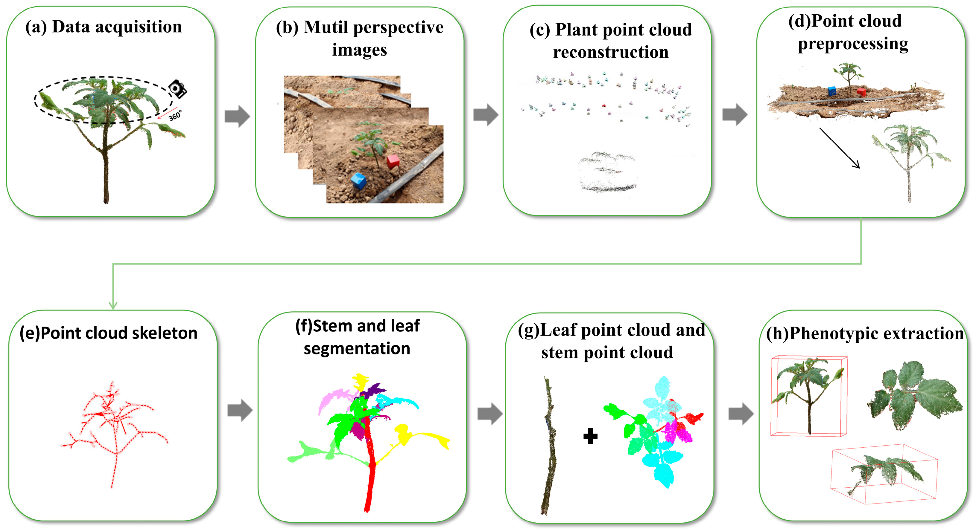
2.1. The Process of the Experiment

The proposed method in this study is illustrated in Figure 1. Firstly, an RGB camera (EOS70D, Canon Corporation, Tokyo, Japan) is used to capture multi-view image data of tomato plants at different growth stages. Secondly, the point cloud of the plant is constructed using OpenMVG + OpenMVS (Version 2.0). Thirdly, the skeleton is extracted from the point cloud after removing noise points. The segmentation of the stem and leaves is achieved by searching for the path of the highest point of the skeleton in the direction of plant growth, combining height and radius constraints, and employing supervoxel clustering based on Euclidean distance. Finally, six phenotypic parameters, namely plant height, stem thickness, leaf inclination, leaf length, leaf width and leaf area, were obtained.

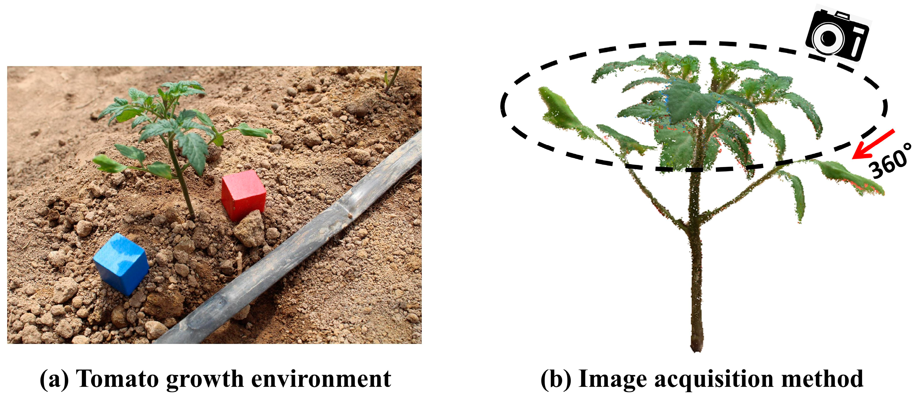
2.2. Image Data Acquisition

The experimental site was the Tomato Industry Research Institute of Shanxi Agricultural University (113°9′34″ E, 40°40′54″ N), and the tomato variety tested was Yuzui 8850. The tomato plants were planted in a solar greenhouse with an area of approximately 1100 m². The greenhouse was equipped with various facilities and equipment for daily management, including wind vents, quilts, water and fertilizer integrated machines, drip irrigation and weather sensors. The spacing between rows was about 50 cm, while the plant spacing was about 40 cm. The tomato seedlings were planted on 15 May 2023. For data collection, a total of 12 tomato plants with uniform light exposure and similar growth in the greenhouse were selected. Point cloud collection experiments were conducted on the 7th, 14th, 21st, 30th, 45th and 60th days after planting. To obtain the scaling factor of the plant point cloud, red and blue calibration blocks with a side length of 3 cm were placed around the tomato (Figure 2a). An RGB camera (EOS70D, Canon Corporation, Tokyo, Japan) was used to capture image data by encircling the tomato plant 360°, as shown in the direction of the red arrow in Figure 2.

For seedling tomatoes, a top-down angle of 45° and lens distance of 30–50 cm from the plant is commonly used to capture images. The shooting angle should be adjusted to ensure that the entire plant is in the frame. As the plant grows, the distance between the lens and the plant should be adjusted accordingly, and the shooting angle should be modified to ensure that the entire plant remains within the frame. As the plant continues to grow, the lower part of the plant may become obstructed. In such cases, it is recommended to take photographs of the upper and lower layers of the plant in 360°. During this process, it is important to ensure overlap between the two parts of the image. This will facilitate the extraction of feature points for subsequent reconstruction and analysis. For tomato plants of different sizes, about 30–100 images are taken to form a multi-view image sequence, and the overlap between two neighboring images should reach 70%. Tomato plants grow very rapidly in the seedling stage and images were taken every 7 days for reconstruction, while, when the growth rate of tomato plants decreased in the later stages, images were taken every 15 days for reconstruction. By adjusting the frequency of image capture according to the growth stage, we can strike a balance between capturing essential data for analysis and monitoring plant development, while optimizing efficiency in the reconstruction process.

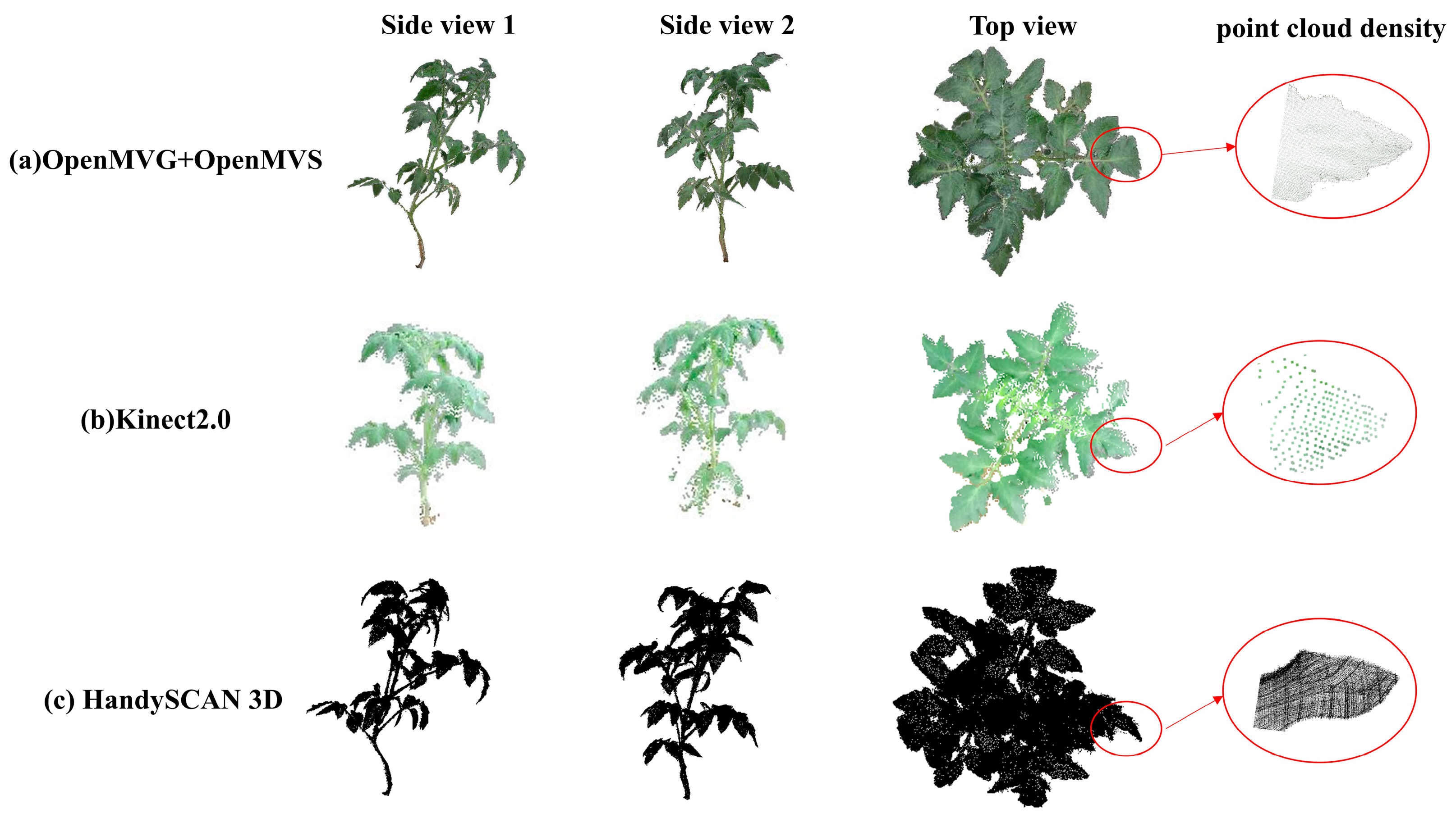
2.3. Point Cloud Reconstruction and Preprocessing

Based on the acquired multi-view image sequence of tomato plants (Figure 3a), the OpenMVG + OpenMVS (Version 2.0) reconstruction method [29] was employed to generate a dense point cloud of the tomato plants (Figure 3b). Finally, a PLY file with color information was generated as the output. However, the reconstructed dense point cloud often contains a significant number of ambient and noise points, which can adversely affect subsequent processing speed and accuracy. Therefore, this study utilized a combination of multiple filtering methods [30] to remove these noise points.

To begin with, the point cloud is traversed to extract the color component of each point. The ultra green component value (EXG) of each point is then calculated using Equation (1). Points having an EXG value below 30 are considered environmental points that need to be filtered out.

$$\mathrm{E}\mathrm{X}\mathrm{G}=2\mathrm{G}-\mathrm{R}-\mathrm{B}$$

(1)

where EXG denotes the value of super green component, and R, G and B denote the red, green and blue color components.

After removing the environmental point cloud, there are still a large number of outlier noise points between the leaf and stem, which are then removed using statistical filtering. The number of neighborhood points n and the standard deviation coefficient α in the statistical filtering are the key parameters of the filtering and, by comparing the filtering results of the combinations of multiple sets of n and α parameters, the discrete and noisy points in the tomato plants can be effectively removed when n = 30 and α = 2.0, and the leaf tips, edges and stems are preserved details (Figure 3c); at the same time, in order to save time in algorithm calculation, voxel filtering was finally adopted to streamline the point cloud data and to improve the efficiency of algorithm calculation, and, when the voxel filtering parameter voxel size was set to 0.03, the streamlining of the point cloud was accomplished without affecting the overall morphology and structure (Figure 3d). The continuous reconstruction of the tomato plants is shown in Figure 3e.

2.4. Stem and Leaf Segmentation Methods

Tomato plants branch in a symbiotic manner, starting at the beginning of flowering when they grow more lateral shoots and branches on the main branch. As the tomato plant grows, the number of stems and leaves within the canopy increases, leading to more significant variability in the morphological performance of different individuals at the same growth stage [31], which makes it difficult to segment by fixed means (e.g., clustering, model fitting, etc.). Thus, this study extracts a stem and leaf segmentation method based on skeleton extraction and supersomal clustering.

According to the tomato morphological structure, tomato organs can be divided into stem point cloud and leaf point cloud. The stem and leaf segmentation method proposed in this study takes the plant point cloud as an input to extract the point cloud skeleton, separates the stem from the leaf through the point cloud skeleton, and finally segments the single leaf through the Euclidean distance-based hyperhomology clustering method.

2.4.1. Skeleton Extraction

A Laplacian contraction-based method [32] was used to extract the tomato plant skeleton. Firstly, Delaunay neighborhood estimation is performed on the input tomato point cloud, and the skeleton point set C is obtained by contracting the Delaunay neighborhood of the original point cloud for several iterations based on the Laplacian operator (Figure 4a); the final undirected graphic point cloud skeleton T is obtained by connecting any two neighboring vertices into an edge through the topological connection method (Figure 4b).

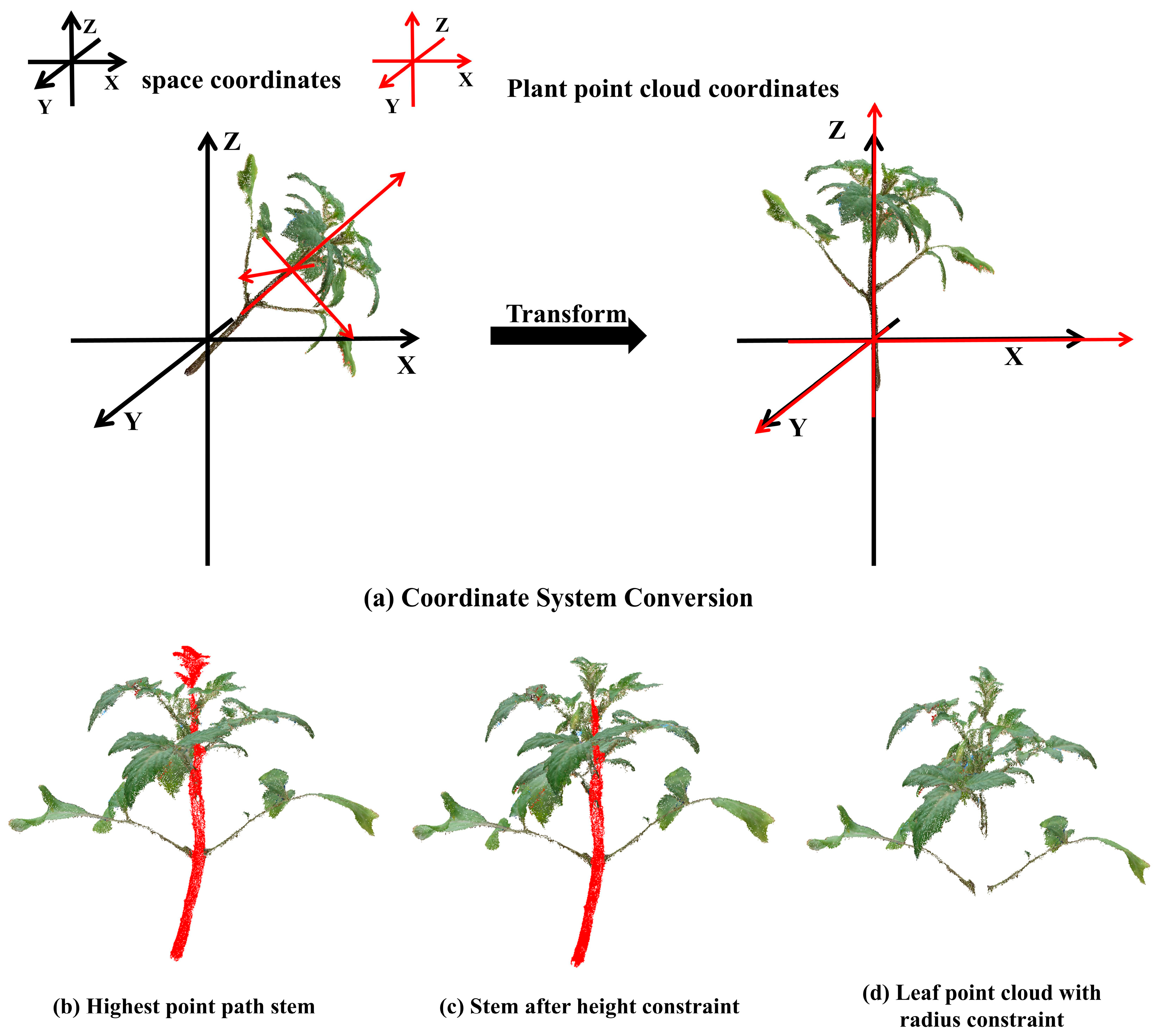
2.4.2. Skeleton Based Stem Extraction

Stem extraction consists of a total of four steps: plant coordinate system correction, finding the path to the highest point of the skeleton, height constraints and radius constraints.

Plant Coordinate System Correction

The relationship between the coordinate system where the reconstructed plant point cloud is located and the spatial coordinate system is random, which is not conducive to subsequent processing. Using principal components analysis (PCA) [33], the coordinate system where the plant skeleton was located was transformed to the spatial coordinate system, and the growth direction of the transformed plant was consistent with the direction pointed by the Z-axis of the point cloud in the spatial coordinate system (Figure 5a).

Finding the Path to the Highest Point of the Skeleton

Firstly, the KdTree search mechanism is used to traverse the entire skeleton point cloud to find the root vertex of the stalks. Subsequently, the Dijkstra algorithm [34] is utilized to find the Minimum Spanning Tree (MST) path [35] from the root vertex of the stalks to the highest connecting point along the growth direction. The path represents the path of the stalk and is fitted to the corresponding point cloud to obtain the stalk point cloud (Figure 5b).

Height Constraint

When searching the path by finding the highest point path, the topmost leaf will be misclassified as a stalk. Due to this problem, the top leaf is removed by the method of height constraint. In the stalk skeleton, we find and arrange the connecting vertices of the stalk skeleton sequentially, traverse these points in reverse to find the connecting vertices between the topmost leaf skeleton and the stalk skeleton, and use the Z-coordinate value of the connecting vertices as the threshold value to remove points larger than the threshold value to obtain the constrained stalk point cloud (Figure 5c).

Radius Constraint

The radius constraint refers to using points larger than the minimum radius of the fitted stalk as leaf points. We treat the stem as a cylinder by default and fit it using the random consistent sampling method (RANSAC) [36], starting from the bottom of the stem and gradually traversing upward through all the stem points to obtain the minimum radius of the fitted cylinder, and presenting the points larger than the minimum radius to obtain a point cloud that is the leaf point cloud (Figure 5d).

2.4.3. Supervoxel Clustering Based on Euclidean Distance

We first segmented the leaves after removing the stalks using the Euclidean distance-based segmentation method [37], and the output cluster of different colors is a single leaf (Figure 6a). However, when the leaves overlap and adhere to each other, there is a situation where two different leaves are grouped together (Figure 6b). By observing that there are more obvious concave and convex mutations between overlapping and adhering leaves, a segmentation method based on supervoxel clustering [38] is used for further segmentation. The point cloud to be segmented is first subjected to supervoxel processing to obtain a supervoxel neighborhood map (Figure 6c). Then, the common edges of the supervoxel neighborhood graph are judged for concavity and convexity using the locally convex connected patches [39] (LCCP) algorithm, as shown in Equations (2) and (3). When C ≥ 0, it is judged as a convex property; otherwise, it is a concave property. The hyperboloid point cloud is reclustered according to the concavity and convexity to realize the segmentation between the adherent blades (Figure 6d).

$$C=n_{1}d-n_{2}d$$

(2)

$$d=\frac{x_1-x_2}{{\Vert x_1-x_2\Vert }_2}$$

(3)

where $n_1$ and $n_2$ are the normal vectors of the two neighboring voxel blocks, and $x_1$ and $x_2$ are the center of mass vectors of the neighboring voxel blocks.

2.5. Phenotype Extraction Method for Tomato Plants

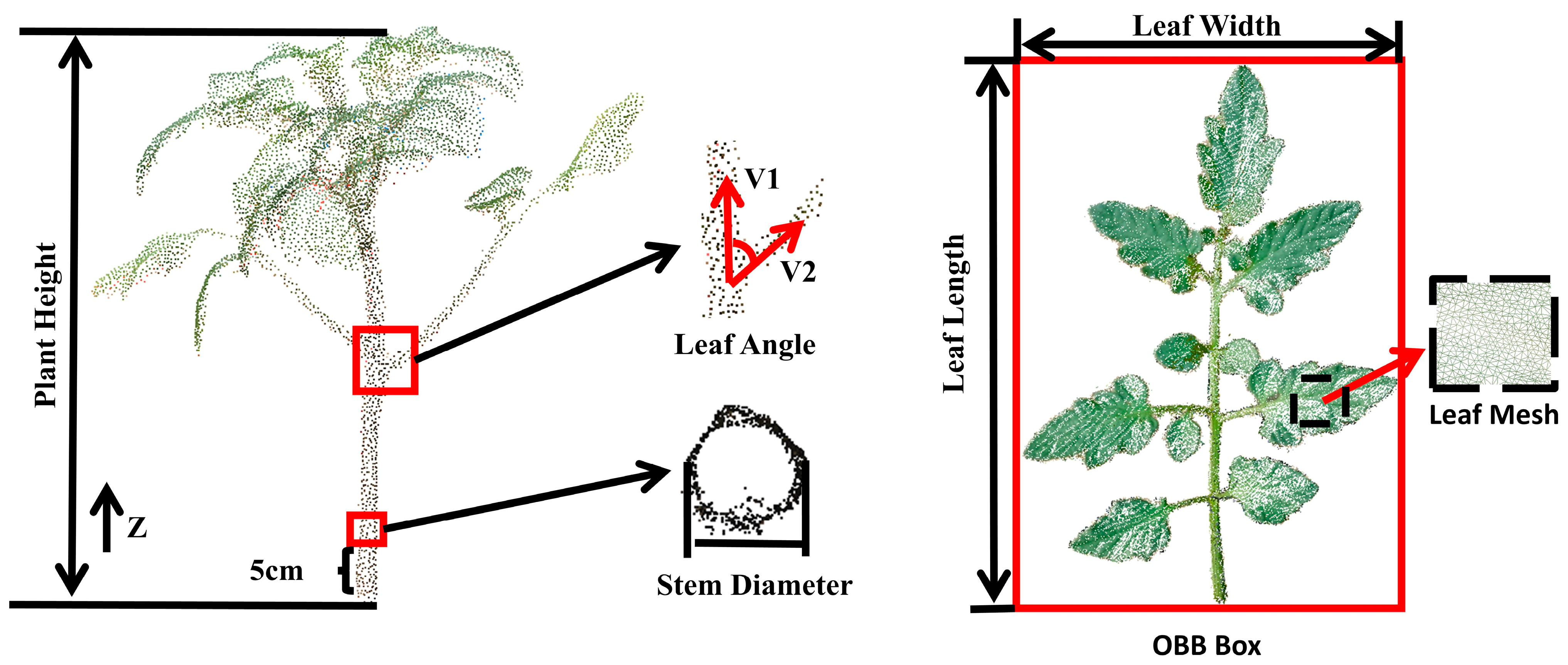
2.5.1. Phenotypic Parameter Extraction Method Based on Point Cloud

A total of six parameters such as plant height, stem diameter, leaf angle, leaf length, leaf width and leaf area were extracted in this study, and the schematic diagram of the extraction is shown in Figure 7.

Plant height and leaf width were obtained by constructing an Oriented Bounding Box (OBB) [40] of the plant, which was determined by the difference between the maximum and minimum coordinate values of the Z-component and X-component directions of the bounding box, respectively.

Leaf length was extracted using an extraction method based on the K-nearest neighbor algorithm (KNN) [41], which finds the two points with the farthest spatial distance as the start and end points, and searches for neighboring points to fit the midvein of the leaf by setting the K-value, and extracts the shortest curve that approximates the midvein on the point cloud of the leaf, i.e., the leaf length.

Stem diameter was determined by unifying the point cloud of the stem at 5 cm above the ground as the location of stem thickness measurement, fitting a circle to the intercepted stem, and the diameter of the fitted circle was the stem thickness.

Leaf angle is the angle between the petiole and the stem; the vector V1 of the stem and the vector V2 of the petiole were extracted, respectively, and the angle between V1 and V2 was calculated as the leaf inclination angle.

Leaf area was obtained by meshing the leaf blade through a greedy projection triangulation algorithm [42] to obtain a number of spatial triangular surface pieces. The total area of the spatial triangular facets was calculated by the Helen’s formula, and the total area obtained was used as the leaf area parameter, which is shown in Equation (4), where $P_i$ denotes one-half of the perimeter of the faceted triangles; a_i, b_i, and c_i denote the lengths of each side of the triangles; $n$ is the total number of triangular facets; and S_leaf denotes the leaf area.

$$S_{\mathrm{leaf}}={\displaystyle \sum _{i=0}^n\sqrt{P_i\left(P_i-a_i\right)\left(P_i-b_i\right)\left(P_i-c_i\right)}}$$

(4)

Since there is a scaling relationship between the 3D model of tomato plant and the actual tomato size, a coordinate scale correction is needed to obtain the scaling coefficient to convert the measured value to the real value. As shown in Equation (5), r is the scaling factor, H_real is the real edge length of the calibration block, and H_{reconstructed} is the edge length of the calibration block point cloud.

$$r=\frac{H_{\mathrm{real}}}{H_{\mathrm{reconstructed}}}$$

(5)

2.5.2. Phenotypic Parameter Real Value Acquisition

The real data measurement of phenotypic parameters involved in this paper was mainly carried out in the following ways, and the manual hand-measured metrics were all repeated three times for the purpose of minimizing errors in the measurements:

• Measurement of real data on plant height: using a tape measure, the distance from the ground part to the highest point of plant growth was measured as the plant height real value;
• Measurement of real data stem diameter: the stem at 5 cm above ground was uniformly selected, vernier calipers were used to measure the longitudinal and transverse distances of the stem using the crossover method, and, finally, the average of the two distances as the real value of the stem diameter was taken;
• Measurement of real data leaf angle: the angle between the leaf ventral surface and plant growth direction was measured with a protractor as the true value of the leaf angle;
• Measurement of real data leaf length: a tape measure was used to measure the distance from the petiole to the tip of the leaf as the true value of the leaf length;
• Measurement of real data leaf width: a tape measure was used to measure the distance of the maximum width of the middle part of the leaf as the true value of the leaf width;
• Measurement of real data leaf area: destructive sampling of the leaf was performed by placing the leaf on a black curtain containing a calibration block, using image processing techniques to extract the contours of the leaf and the calibration block, respectively, solving for their respective pixel points, and performing a pixel conversion to obtain the true leaf area of the leaf (Figure 8).

2.6. Evaluation of Stem and Leaf Segmentation and Phenotype Extraction

Stem and leaf segmentation segments the number of leaf point clouds to evaluate its segmentation effect; the number of organs belonging to leaf point clouds that were segmented correctly is denoted by TP, the number of organs belonging to leaf point clouds that were not segmented successfully is denoted by FN, and the number of non-leaf point cloud organs that were segmented as leaf point clouds is denoted by FP. Based on the above three parameters, we calculated the accuracy rate (Precision, P), recall rate (Recall, $R$) and F1-score (F1-score, $F_1$). The calculations are shown in Equations (6)–(8).

$$P=\frac{TP}{TP+FP}$$

(6)

$$R=\frac{TP}{TP+FN}$$

(7)

$$F_1=\frac{2\times P\times R}{P+R}$$

(8)

The phenotype extraction parameters were acquired using the linear regression method for evaluation, and the coefficient of determination (R²) between the measured and actual values of the point cloud and the root mean square error (RMSE) were calculated to assess the error and accuracy of each parameter, which were calculated as in Equations (9) and (10).

$$R^2=\frac{{\sum }_{i=1}^n\left(X_i-\overline{X}\right)\left(Y_i-\overline{Y}\right)}{\begin{array}{cc}\sqrt{{\sum }_{i=1}^n{\left(Y_i-\overline{Y}\right)}^2}& \sqrt{{\sum }_{i=1}^n{\left(X_i-\overline{X}\right)}^2}\end{array}}$$

(9)

$$RMSE=\sqrt{\frac{1}{n}{\displaystyle \sum _{\mathrm{i}=1}^n{\left(X_i-Y_i\right)}^2}}$$

(10)

where X_i and Y_i are the ith real and calculated values, respectively, and are the average of the real and calculated values, respectively, and n is the total number of real or calculated values.

3. Results

3.1. Effectiveness and Evaluation of Different Stages of Stem and Leaf Division

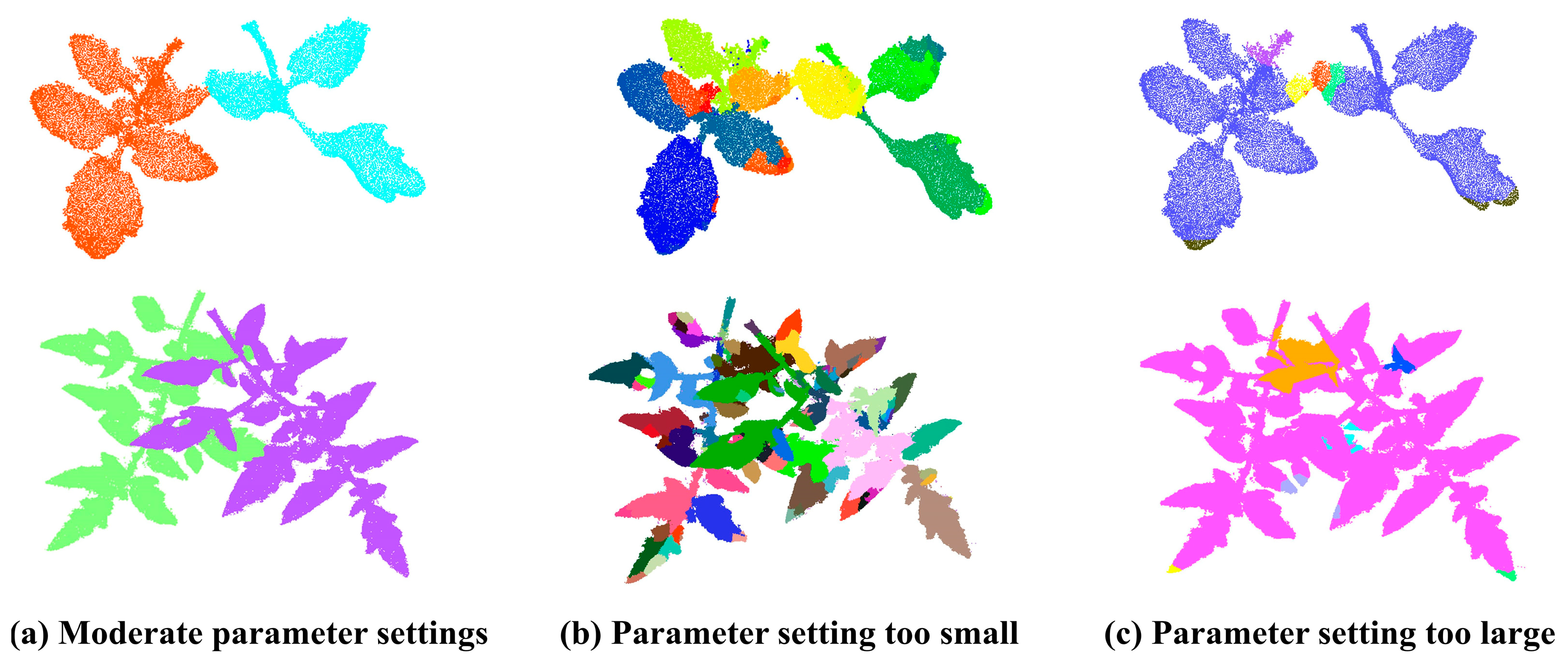
3.1.1. Effect of Algorithm Parameters on Blade Segmentation Accuracy

The parameters affecting the effect of leaf segmentation are seed resolution Rseed, voxel resolution Rvoxel and minimum segmentation size Smin. It was found that Rseed determines the size of the voxel region, and the larger the value of Rseed, the fewer the voxels, resulting in smaller differences between neighboring pixels; however, the smaller the value of Rseed, the more the voxels, which results in a decrease in the efficiency of the algorithm. Rvoxel mainly determines the resolution of voxel generation; when Rvoxel is too small, the resolution is too large to generate a complete voxel neighbor map; when Rvoxel is too large, the resolution will be reduced, resulting in missing features. The main parameter affecting the accuracy of supervoxel segmentation is Smin; if set too small, it will cause the blade to be over-segmented into multiple parts, and, if set too large, it will lead to a lack of segmentation, which cannot meet the actual segmentation requirements.

By comparing the results of several tests, the parameter value with optimal segmentation effect is selected. For the case that there is a small part of adhesion between two blades, the parameters are set as Rseed = 0.15, Rvoxel = 0.05 and Smin = 0.2, which can achieve a better segmentation effect. For the case where there is a large part of overlap between two leaves, the point cloud is denser due to the larger adhesion area and the value of the parameter should be increased appropriately according to the size of the adhesion area, and a better segmentation effect can be achieved when the parameter is set to Rseed = 0.35, Rvoxel = 0.1 and Smin = 0.35 (Figure 9a). When the parameters are set too small (Rseed = 0.05, Rvoxel = 0.01, Smin = 0.1 and Rseed = 0.25, Rvoxel = 0.05, and Smin = 0.3), it leads to the generation of too many supervoxel blocks, which requires more concavity and convexity judgments, resulting in a longer algorithmic computation time, and also results in the over-segmentation of the blades (Figure 9b). With too-large parameter settings (at Rseed = 0.25, Rvoxel = 0.1, Smin = 0.3 and Rseed = 0.45, Rvoxel = 0.15, and Smin = 0.4), the number of supervoxels decreases, and the number of concavity and convexity features between neighboring voxel blocks decreases, which does not allow the judgment of enough features for segmentation, and tends to result in the under-segmentation of the leaf (Figure 9c).

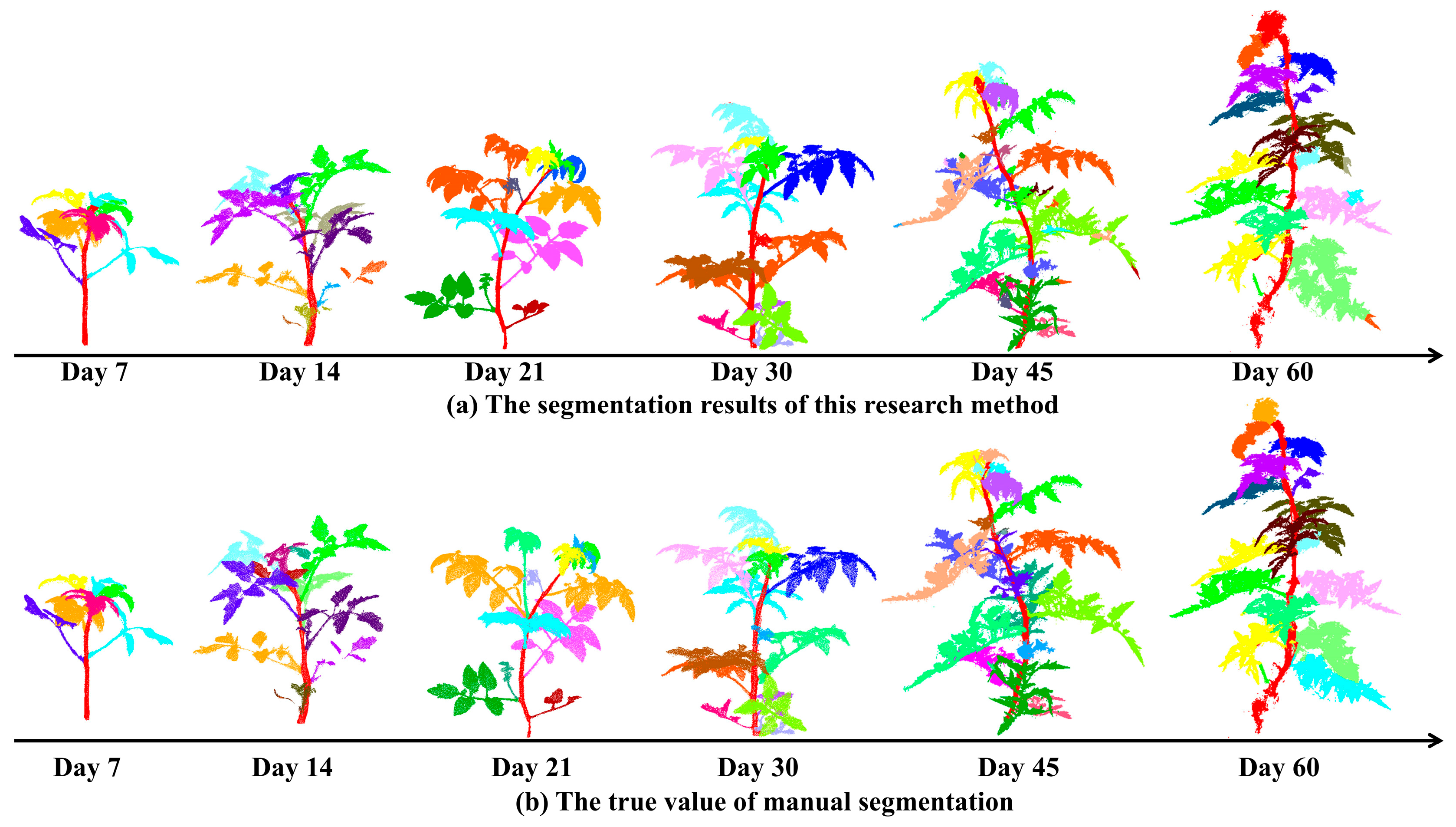
3.1.2. Stem and Leaf Segmentation Effect

In this study, stem and leaf segmentation of 12 tomato plants each at 7, 14, 21, 30, 45 and 60 days after planting was used to evaluate the segmentation results of the present study method, and the visualization results for different growth days are shown in Figure 10a. Meanwhile, the real values of stem and leaf segmentation of tomato plants were obtained by manual segmentation by Cloud compare software (Version 2.10.1; GPL) [43]. The effect of manual segmentation is shown in Figure 10b, which was used to compare the differences between the segmentation results of the algorithm of this study and the real values. Through comparison, we found that the overall segmentation of tomato plants using the algorithm of this study is more effective, but the following situations will cause segmentation failure:

(1)

As the plant grows, side shoots grow between the leaves and the stem, and our algorithm does not effectively segment them from the leaves, causing the side shoots and leaves to be grouped together, resulting in under-segmentation;

(2)

When there is a break between the leaves, our algorithm will split that leaf into multiple parts, obtaining many incomplete leaves, resulting in over-segmentation;

(3)

When there are mostly adhesions and occlusions between the blades, it is not possible to perform a complete segmentation by adjusting the parameters of the supervoxel, and, due to the large differences in the normal vectors between such leaves, it is unavoidable that the segmentation of a leaf into multiple parts occurs, resulting in an increase in the final number of leaves.

The accuracy of leaf segmentation in tomato plants with different days of growth is shown in

Table 1. Precision of stem and leaf segmentation in tomato plants on different growth days.

Growth Days/d	$\mathit{P}$	$\mathit{R}$	${\mathit{F}}_1$
7	0.88	0.80	0.84
14	0.91	0.84	0.87
21	0.92	0.85	0.88
30	0.88	0.82	0.85
45	0.86	0.77	0.81
60	0.84	0.74	0.79
Average	0.88	0.80	0.84

. The accuracy and recall of leaf segmentation on the 7th, 14th and 21st days after planting were 0.88, 0.91 and 0.92, and 0.80, 0.84 and 0.85, respectively, and both the accuracy and recall increased gradually with plant growth. The increase in accuracy was due to the dense growth of the apical structure of tomato in the seedling stage, and the occurrence of mistaken classification of the top leaf centers or incompletely unfolded leaflets as leaves, which led to lower accuracy. This resulted in a lower accuracy rate, which was alleviated as the top compactness decreased with growth; the recall rate was somewhat affected by the segmentation of some leaves due to their sagging and cross-growth. However, with the increasing leaf spacing, the crossing situation was reduced, which was more favorable for the segmentation of extracted leaves.

However, the segmentation accuracy and recall on the 30th, 45th and 60th days after planting began to decrease, which were 0.88, 0.86 and 0.84, and 0.82, 0.77 and 0.74, respectively, which indicated that with the growth of the plant, on the one hand, the lateral buds produced at the petiole were mistakenly treated as leaves and segmented at the same time, resulting in mis-segmentation, and, on the other hand, due to the oversized leaf morphology, segmentation of leaves by the concavity algorithm will result in single leaf over-segmentation, and the over-segmented part will be categorized as a new leaf, which leads to a decrease in the accuracy; meanwhile, the decrease in the recall rate indicates that, with the growth of the plant, the plant shape is too large, and the overlap of the leaves is significant, which makes it difficult to segment them.

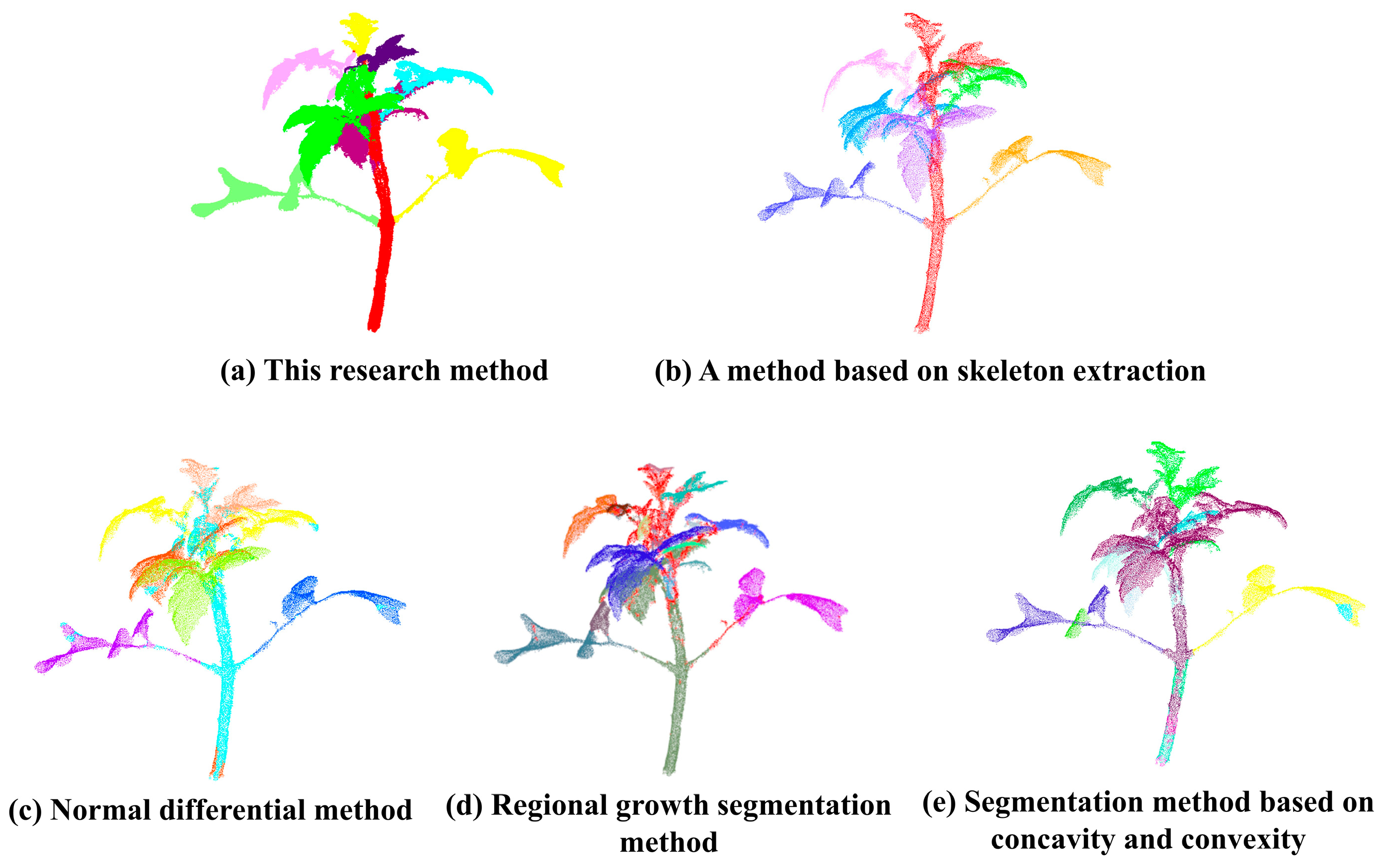
3.1.3. Comparison of Different Segmentation Methods

In order to verify the accuracy of the segmentation algorithm in this study, we compared the segmentation effect of the stem and leaf segmentation algorithm proposed in this study with four commonly used segmentation algorithms, including the skeleton extraction-based segmentation method [28], the normal differential difference method [20], the region growing method [22] and the concavity-based segmentation method [39], and the segmentation results of different algorithms are shown in Figure 11.

The method based on skeleton extraction has a better segmentation effect on leaves without adhesion occlusion, but has a poorer segmentation effect on leaves at the tip of stalks, which categorizes the apical leaves with stalks; at the same time, due to the phenomenon of skeleton offset that occurs when extracting the skeleton, some of the petiole of the leaf blade is classified as stalk, which results in the part of the leaf blade being missing, affecting the results of the subsequent measurements. The normal differential difference method, regional growth segmentation method and concavity-based segmentation method only use parameters such as curvature threshold, distance threshold and normal information as the basis of segmentation, which are more effective for segmentation of a single blade and a part with obvious concave and convex features, but when facing the situation where the distance between the leaf blade and the stem is close, the leaf blade and part of the stem will be divided together, which results in the leaf blade and the stem not being able to be completely segmented, and there is a phenomenon of excessive segmentation and an under-segmentation phenomenon.

The comparison results of the stem and leaf segmentation accuracy of the five methods are shown in

Table 2. Comparison of stem and leaf segmentation accuracy among five methods.

Methods	Average of Precision	Average of Recall Rates	Average of F1
This research method	0.88	0.80	0.84
Segmentation method based on skeleton extraction	0.77	0.63	0.76
Normal differential method	0.64	0.59	0.57
Regional growth segmentation method	0.58	0.53	0.59
Segmentation method based on concavity and convexity	0.54	0.57	0.62

; the proposed method of stem and leaf segmentation has the best segmentation effect, and all the indexes are higher than the other four methods. Compared with the other methods, the average segmentation accuracy of this method is improved by 11, 24, 30 and 34 percentage points, respectively, which indicates that the stem and leaf segmentation method constructed in this study is more suitable for the point cloud segmentation of tomato plants.

3.2. The Present Study on the Effectiveness of Stem and Leaf Division Methods for Division in Different Crops

In order to prove the generalization ability of the stem and leaf segmentation method of this study, a total of five greenhouse crops, namely maize, eggplant, cucumber, pepper and squash, were selected as test objects in this study and six plants of each crop were selected for the test. The effect of stem and leaf segmentation of the different crops is shown in Figure 12, which shows that effective segmentation can be carried out for different crops as well.

The average segmentation values for each crop are shown in

Table 3. Average segmentation results of different greenhouse crops.

Crop Name	Average of Precision	Average of Recall Rates	$\mathbf{Average} \mathbf{of} {\mathit{F}}_1$-Score
Maize	0.98	0.96	0.94
Eggplant	0.97	0.95	0.96
Cucumber	0.97	0.94	0.97
Pepper	0.95	0.93	0.92
Squash	0.92	0.89	0.92

, and the average accuracies for the five crops are 0.98, 0.97, 0.97, 0.95 and 0.92, with segmentation accuracies above 90%, indicating that the stem and leaf segmentation method of the present study has a certain degree of generalization, and it can be effectively applied to stem and leaf segmentation work for other crops.

3.3. Phenotypic Parameter Measurement Results

The results of the assessment of the measured values of each phenotypic parameter in comparison with the measured values are shown in Figure 13.

The evaluation results showed that there was a high correlation between the plant height extracted by the method of this study and the manual measurements, with an R² and $RMSE$ of 0.97 and 2.17 cm, respectively, reflecting that the measurements of the method of this study were very close to the manual measurements, and the plant height could be accurately measured using the method of this study.

The results of leaf length, leaf width and leaf area measured by the present study method showed a strong correlation and small error between the results and the manual measurements, and the R² and $RMSE$ of leaf length, leaf width and leaf area were 0.94, 0.92, 0.93 and 3.18 cm, and 2.99 cm and 8.79 cm², respectively, which indicated that the present study method could also accurately measure the leaf-related parameters with good robustness.

The $R^2$ and $RMSE$ between stem diameter and leaf angle extracted by the method of this study and the manual measurements were 0.84, 0.346 cm and 0.88, and 5.65°, respectively, and the correlation coefficients of both traits were lower than 90%, and the measurement errors were high relative to the other phenotypic parameters, which suggests that there is still a lot of room for subsequent improvement.

3.4. Algorithm Efficiency Evaluation

In this study, we used a consumer-grade RGB camera to capture image data of tomato plants, and a total of 30–100 images were captured for tomato plants with different numbers of growth days. The captured images were fed into the OpenMVG + OpenMVS algorithm for reconstruction, followed by preprocessing, stem and leaf segmentation, and phenotype extraction steps. All the algorithms used in this study were on a server with an environment configuration of 13th Gen Intel (R) Core (TM) i7-13700KF 3.40 GHz, 64 G RAM, and NVIDIA GeForce RTX 4080 24 GB GPU for graphics. In order to evaluate the efficiency of the algorithm in this study, the time spent on point cloud reconstruction, stem and leaf segmentation (including preprocessing), and phenotype extraction was recorded for a total of 60 tomato plants with different growth days, and the average processing time was calculated to facilitate the evaluation of the algorithm efficiency, and the statistics of the average time spent on the algorithm operation are shown in

Table 4. Algorithm efficiency statistics.

Processing Stage	Point Cloud Reconstruction/min	Stem and Leaf Segmentation/min	Phenotypic Extraction/min	Total Time/min
Minimum processing time	7.37	3.26	1.72	12.35
Maximum processing time	26.44	7.26	3.59	37.29
Average processing time	17.89	5.25	2.97	26.11

.

When the plants were in the seedling stage, a total of about 30 images were taken, and it took about 7 min to reconstruct them; as the tomato plants grew, it took about half an hour to reconstruct them, and the average reconstruction time for the 60 tomato plants was 20.89 min. The average processing time for the stem and leaf segmentation was 6.25 min, of which 80% of the time was spent in the pre-processing and skeleton extraction, which took a minimum of 2.61 min and a maximum of 5.8 min, depending on the plant size. The minimum processing time was 2.61 min, while the maximum processing time was 5.8 min, and the processing speed of this part was very closely related to the size of the strain. In the phenotypic parameter extraction part, the average time was 2.97 min, and the number and size of leaves were more related to the processing time, the more the number of leaves and the larger the leaves, the larger the calculation volume of the algorithm, resulting in a corresponding increase in the calculation time. Therefore, the time consumed to complete the reconstruction, stem and leaf segmentation, and phenotype extraction of a tomato plant was at least 12.35 min, at most 37.29 min, and the average time was 30.11 min. Among all the processes, plant reconstruction took the most time, which accounted for about 70% of the total time spent. This was mainly due to the complex structure of tomato plants with severe branch and leaf occlusion; the lack of plant point cloud details can be further compensated for by increasing the number of images, and more advanced computer configurations can be used subsequently to further improve the reconstruction efficiency. The tomato plant reconstruction and phenotype extraction method proposed in this study takes about 62.5% less time and is more computationally efficient compared to the method used in the literature [27].

4. Discussion

4.1. Comparison of Three-Dimensional Weighting Methods

According to the existing conditions, this study chooses three ways to reconstruct the plants, the method used in this study, reconstruction using an RGB-D camera (Kinect 2.0) and reconstruction using a structured light scanner (HandySCAN 3D), to compare the accuracy of the point cloud reconstruction, the cost, the efficiency of the data collection and the scene of the data collection, respectively. The point clouds reconstructed by the three methods are shown in Figure 14.

The Kinect 2.0 camera is widely used in indoor and outdoor agricultural production due to its relatively low price and efficient imaging method [9,31,42]. In this study, a three-view point cloud of the plant was acquired using a Kinect 2.0 camera and reconstructed using the point cloud alignment method, and the reconstructed point cloud is shown in Figure 14b. The accuracy of the reconstructed point cloud is poor compared to the method in this study, and there are a large number of discrete points in the periphery, and the point cloud is scattered, which greatly increases the difficulty of subsequent processing. At the same time, the camera is greatly affected by light, and strong light exposure will cause a serious lack of plant point cloud, affecting the results of the subsequent strategic measurements.

The point cloud generated by the structured light scanner is shown in Figure 14c, which has a higher accuracy and more uniform local density of the point cloud, reducing the difficulty of post-processing and realizing high-throughput data acquisition [10,11]. However, the disadvantages are that the point cloud reconstructed by this scanner has no color information and cannot be processed by color information, and the expensive price of this scanner limits its wide application. Compared with the point cloud reconstructed by the method used in this study, the structured light scanner has better visualization, is more automated and is more costly. When using this method to construct a plant point cloud, the plant needs to be placed on a specific carousel, which places a limitation on the size of the plant and is affected by light, and the point cloud reconstruction must be undertaken indoors in a relatively ideal environment.

Considering the accuracy, cost and processing rate, the method in this study has high reconstruction accuracy and can be processed according to the color information, which greatly improves the processing efficiency; moreover, the cost is low, and the reconstruction can be carried out with only one RGB camera to collect the data, which greatly increases the practicability, and it is more suitable to be used for the three-dimensional reconstruction of the plant and the extraction of the phenotypes.

4.2. Stem and Leaf Segmentation

Tomato has a more complex topology compared with corn, sorghum, soybean and other crops; due to the complexity of the topology, it is difficult to finely separate stalks and leaves by means of clustering [20,21,22], which will result in the adhesion between leaves and stalks, causing too much missegmentation. The methods of model fitting include fitting cylinders [23] and fitting spheres [24], but in the case of tomato, the stalks are not regular columns, and the fitting will misclassify. Some leaves are misclassified as stalks, and it is also impossible to completely separate stalks from leaves; although the segmentation methods based on deep learning [25,26] have achieved better results, the existing research is mainly aimed at seedling crops, and the segmentation effect is still unsatisfactory for later crops with larger plants, and this type of method requires a high computer configuration and a large amount of manual hand labeling, which greatly reduces the work efficiency.

Skeleton information is a simple structural representation of the model, which can reflect the topological structure of the model, as well as the morphological characteristics, and help to realize the growth simulation of crops. In this study, for tomato plants with complex topology, the skeleton extraction method based on the Laplace algorithm is used to extract the plant skeleton, and the stalks are searched by determining the path of the highest point of the skeleton and combined with supersomal clustering to complete the segmentation of a single leaf, which obtains better results. The average accuracy, recall and F1 score of segmentation were 0.88, 0.80 and 0.84, respectively, which improved the average accuracy by 11, 24, 30 and 34 percentage points compared to several methods in Section 3.1.3. Generalizability tests were also conducted for the remaining five seedling crops, and all of them achieved better segmentation results.

However, the method in this study caused a decrease in segmentation accuracy with plant growth, mainly due to the following reasons: on the one hand, the organs of tomato plants gradually mature, and the lateral buds also grow at the intersection of stalk and petiole, which makes the overlap more serious and the spatial structure more complicated; on the other hand, due to the limitation of plant size, the point cloud of the plant has different degrees of error, which leads to the existence of organs sticking together and blurred outlines inside the plant. These problems greatly affect the skeleton extraction, and it is easy to divide the path of the highest point of the stalk skeleton to the direction of leaf extension when searching for the skeleton, forming a closed loop of the skeleton. Through subsequent attempts to improve the skeleton extraction algorithm accordingly by introducing streamline curvature into the skeleton extraction algorithm [44], a structurally complete, continuous, loop-free and reasonably oriented crown skeleton can be extracted.

4.3. Extraction of Phenotypic Parameters

Using the measurement method in this study, the correlation between the measurement results and the manually measured values was high. However, there were still errors due to some unavoidable reasons.

The error in plant height mainly came from the plant’s fall; we could not recognize the highest point of the plant accurately, which caused the measurement error in plant height.

There are two main factors that lead to the measurement error in leaf length, leaf width and leaf area: (1) in the single-leaf segmentation, the use of supervoxel clustering will put some of the leaf tip or the inner leaf point cloud into another category, resulting in the extraction of some measurements that are too large; (2) in the situation where the leaf is heavily shaded, the heavy shade will lead to the reconstruction of the details of the shaded part being incomplete. Segmentation will also result in too small phenotypic measurements due to missing leaves. Both of the above aspects can lead to the situation of missing leaves, resulting in too large or small leaf-related phenotypic parameter measurements.

The reason for the error in stem thickness is that, when measuring, we fit the cross-section of the stem to a circle and take the diameter of the fitted circle as the stem thickness, but, as tomato grows, the cross-section of the stalk may be more similar to an ellipse, and the actual measured distance is closer to the length of the short axis of the ellipse, thus causing an error; when measuring leaf inclination, the overlapping of leaf blades leads to the petiole vector being offset, which produces certain results in the measurement of leaf inclination. The results of the leaf inclination angle measurement will have certain results.

4.4. Future Work

The method of this study has the advantages of non-contact and high accuracy compared with the traditional measurement method, which reduces the error and work intensity of manual measurement and provides technical support for organ segmentation and high-throughput phenotyping of multi-branch crops such as tomato. However, this study also has some limitations:

(1)

First, this study still acquires image data manually, which cannot be fully automated, and we will consider the combination of multiple cameras and mobile devices to realize the automatic acquisition of image data in a later stage;

(2)

Second, for the segmentation failure caused by mutual organ occlusion, the algorithm used will be subsequently improved to further increase the segmentation accuracy;

(3)

Third, the missing leaves seriously affected the phenotypic measurement results, and the point cloud complementation will be considered at a later stage to complement the mutilated leaves to further improve the measurement accuracy of the phenotypic parameters;

(4)

Finally, new methods will be further developed for phenotypic measurements of other organs of the tomato plant, such as fruits, roots, nodes and flowers, to provide a comprehensive picture of tomato growth dynamics. At the same time, according to the pattern of change in phenotypic parameters, there should be work with the water and fertilizer machine, to achieve automatic decision-making and irrigation.

5. Conclusions

The point cloud model of tomato plants at different growing days was constructed, and the method of tomato stem and leaf segmentation and phenotypic parameter measurement was proposed. The following conclusions can be drawn from the analysis of the experimental results:

(1)

Using the stem and leaf segmentation method proposed in this study to test tomato plants with different numbers of growth days, the average accuracy, average recall and average F1 score of stem and leaf segmentation were 0.88, 0.80 and 0.84, respectively, compared with the manual segmentation results; compared with the segmentation methods based on the skeleton, the normal differential difference method, the regional growth method and the segmentation method based on the concavity, the stem and leaf segmentation was successful. The average accuracy rate increased by 11, 24, 30 and 34 percentage points, respectively, indicating that the present research method can segment tomato organs more accurately. Meanwhile, segmentation tests were carried out on five other greenhouse crops, and the average accuracy rates were 0.98, 0.97, 0.97, 0.95 and 0.92, respectively, which had a certain degree of generalization, suggesting that the present research method can be effective in segmenting other crops as well. The method of this study has some reference value in the organ segmentation of multi-branched crops.

(2)

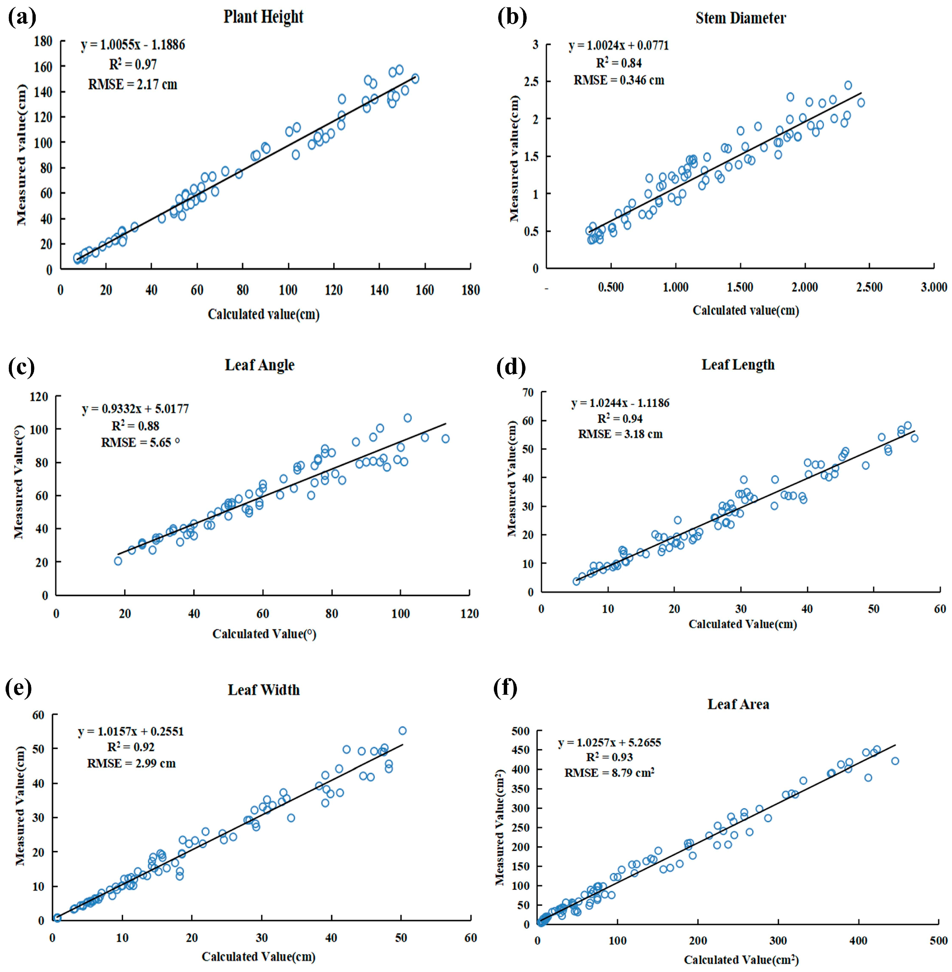
The correlation coefficients (R²) between the phenotype parameters measured using the proposed method and the true values obtained from manual measurements were 0.97 for plant height, 0.84 for stem diameter, 0.88 for leaf angle, 0.94 for leaf length, 0.92 for leaf width and 0.93 for leaf area. The relative errors (RMSE) were 2.17 cm for plant height, 0.346 cm for stem diameter, 5.65 degrees for leaf angle, 3.18 cm for leaf length, 2.99 cm for leaf width and 8.79 cm² for leaf area. The algorithm’s measurement results exhibited a high correlation with the true values obtained from manual measurements, meeting the requirements for agricultural production.

(3)

The average elapsed time of the algorithm used in this study was 26.11 min, which can complete the point cloud reconstruction, stem and leaf segmentation, and phenotype extraction work faster, with high timeliness.

The results show that the proposed method can quickly and accurately complete the stem and leaf segmentation and phenotype extraction of tomato plants. Accurate phenotypic parameters can better optimize a water and fertilizer management strategy to make it more refined and efficient, paired with a water and fertilizer machine for real-time and accurate automatic irrigation; technical support is provided for automatic irrigation of water and fertilizer machines in solar greenhouses at a later stage. This may lead to further improvements in fruit yield and quality, as well as productivity and economic benefits for farmers.

References

1. Chitwood-Brown, J.; Vallad, G.E.; Lee, T.G.; Hutton, S.F. Breeding for Resistance to Fusarium Wilt of Tomato: A Review. Genes 2021, 12, 1673. [Google Scholar] [CrossRef] [PubMed]
2. Roohanitaziani, R.; de Maagd, R.A.; Lammers, M.; Molthoff, J.; Meijer-Dekens, F.; van Kaauwen, M.P.; Bovy, A.G. Exploration of a resequenced tomato core collection forphenotypic and genotypic variation in plant growth and fruit quality traits. Genes 2020, 11, 1278. [Google Scholar] [CrossRef]
3. Shakoor, N.; Lee, S.; Mockler, T.C. High throughput phenoty** to accelerate crop breeding and monitoring of diseases in the field. Curr. Opin. Plant Biol. 2017, 38, 184–192. [Google Scholar] [CrossRef]
4. Huichun, Z.; Meng, Z.; Liming, B. Plant chlorophyll content estimation and visualization technology based on YOLO v5. J. Agric. Mach. 2022, 53, 313–321. [Google Scholar]
5. Lu, C.P.; Liaw, J.J.; Wu, T.C.; Hung, T.F. Development of a mushroom growth measurement system applying deep learning for image recognition. Agronomy 2019, 9, 32. [Google Scholar] [CrossRef]
6. Wang, D.; Li, C.; Song, H.; Xiong, H.; Liu, C.; He, D. Deep learning approach for apple edge detection to remotely monitor apple growth in orchards. IEEE Access 2020, 8, 26911–26925. [Google Scholar] [CrossRef]
7. Lu, J.; Yubin, L.; Zhiyun, W. Optimization of Plant 3D Modeling ICP Point Cloud Registration. J. Agric. Eng. 2022, 38, 183–191. [Google Scholar]
8. Yang, J.; Kai, T.; Weiguo, Z.; Xia, Y. Separation of stems and leaves of gramineous plants in mudflat wetlands from ground lidar point cloud data. China Laser 2022, 49, 122–130. [Google Scholar]
9. Haibo, C.; Shengbo, L.; Lele, W.; Chang, Z. Automated 3D reconstruction and validation of single plant crops based on Kinect V3. J. Agric. Eng. 2022, 38, 215–223. [Google Scholar]
10. Liu, X.; Wang, Y.; Kang, F.; Yue, Y.; Zheng, Y. Canopy parameter estimation of Citrus grandis var. Longanyou based on Lidar 3d point clouds. Remote Sens. 2021, 13, 1859. [Google Scholar] [CrossRef]
11. Zhenghe, Y.; Chen, Y.; Huimin, Y.; Xhou, X. Extraction of geometric parameters of greenhouse tomato canopy based on LiDAR. Xinjiang Agric. Sci. 2021, 58, 1909. [Google Scholar]
12. Jinqi, J.; Jingjing, H.; Jingxin, X. Acquisition of citrus canopy structure information based on mobile 3D LiDAR. J. Hunan Agric. Univ. 2022, 48, 109–113. [Google Scholar] [CrossRef]
13. Lin, C.; Hu, F.; Peng, J.; Wang, J.; Zhai, R. Segmentation and stratification methods of field maize terrestrial LiDAR point cloud. Agriculture 2022, 12, 1450. [Google Scholar] [CrossRef]
14. Jin, S.; Su, Y.; Wu, F.; Pang, S.; Gao, S.; Hu, T.; Guo, Q. Stem-Leaf Segmentation and Phenotypic Trait Extraction of Individual Maize Using Terrestrial LiDAR Data. IEEE Trans. Geosci. Remote Sens. 2019, 57, 1336–1346. [Google Scholar] [CrossRef]
15. Yuchao, L. Research on 3D Reconstruction and Phenotypic Measurement of Maize Plants at Seedling Stage Based on Multi Perspective Images; Hebei Agricultural University: Hebei, China, 2022. [Google Scholar]
16. Johann, C.R.; Stefan, P.; Heiner, K. Accuracy Analysis of a Multi-View Stereo Approach for Phenotyping of Tomato Plants at the Organ Level. Sensors 2015, 15, 9651–9665. [Google Scholar]
17. Shaochen, L.; Aiwu, Z.; Xizhen, Z.; Jang, Z.; Li, M. Method for extracting three-dimensional phenotypic information of maize seedlings at leaf scale. Prog. Laser Optoelectron. 2023, 60, 71–79. [Google Scholar]
18. Chai, H.; Shao, K.; Yu, C.; Shao, J.; Wang, R.; Sui, Y.; Bai, K.; Liu, Y.; Ma, W. Extraction of Beet Root Phenotypic Parameters and Root Type Discrimination Based on 3D Point Cloud. J. Agric. Eng. 2020, 36, 181–188. [Google Scholar]
19. Aobo, J.; Tianhao, D.; Yan, Z. Identification of tobacco plant type features in the field based on 3D point clouds and ensemble learning. J. Zhejiang Univ. 2022, 48, 393–402. [Google Scholar]
20. Yitong, X.; Shuai, L.; Chenlian, H.; Liu, Q.; Li, F.; Zhang, W. Organ segmentation and phenotype analysis of soybean plants based on three-dimensional point clouds. China J. Agric. Sci. Technol. 2023, 25, 115–125. [Google Scholar] [CrossRef]
21. Li, D.; Shi, G.; Kong, W.; Wang, S.; Chen, Y. A leaf segmentation and phenotypic feature extraction framework for multiview stereo plant point clouds. IEEE J. Sel. Top. Appl. Earth Obs. Remote Sens. 2020, 13, 2321–2336. [Google Scholar] [CrossRef]
22. Elnashef, B.; Filin, S.; Lati, R.N. Tensor-based classification and segmentation of three-dimensional point clouds for organ-level plant phenoty** and growth analysis. Comput. Electron. Agric. 2019, 156, 51–61. [Google Scholar] [CrossRef]
23. Xu, Y. Research on Crop Phenotypic Parameter Acquisition and Dynamic Quantification Method Based on Multitemporal Point Cloud Data; Huazhong Agricultural University: Wuhan, China, 2019. [Google Scholar] [CrossRef]
24. Qibing, Z.; Li, H.; Chen, Z. Recognition and counting method of potted kumquat fruits based on point cloud alignment. J. Agric. Mach. 2022, 53, 209–216. [Google Scholar]
25. Li, D.; Shi, G.; Li, J.; Zhang, S.; Xiang, S.; Jin, S. PlantNet: A dual-function point cloud segmentation network for multiple plant species. ISPRS J. Photogramm. Remote Sens. 2022, 184, 243–263. [Google Scholar] [CrossRef]
26. Guo, X.; Sun, Y.; Yang, H. FF-Net: Feature-Fusion-Based Network for Semantic Segmentation of 3D Plant Point Cloud. Plants 2023, 12, 1867. [Google Scholar] [CrossRef] [PubMed]
27. Wang, Y.; Hu, S.; Ren, H.; Yang, W.; Zhai, R. 3DPhenoMVS: A Low-Cost 3D Tomato Phenotyping Pipeline Using 3D Reconstruction Point Cloud Based on Multiview Images. Agronomy 2022, 12, 1865. [Google Scholar] [CrossRef]
28. Cheng, P.; Shuai, L.; Yanlong, M. Tomato plant stem and leaf segmentation and phenotypic feature extraction based on 3D point cloud. J. Agric. Eng. 2022, 38, 187–194. [Google Scholar]
29. Baiming, L.; Qian, W.; Jie, W.; Su, H. Optimization of crop 3D point cloud reconstruction strategy based on multi view automatic imaging system. J. Agric. Eng. 2023, 39, 8675. [Google Scholar]
30. Xiuying, L.; Fengran, Z.; Huan, C.; Fan, B.; Li, H. 3D reconstruction and trait extraction of maize plants based on motion recovery structure. J. Agric. Mach. 2020, 51, 209–2019. [Google Scholar]
31. Zhu, T.; Ma, X.; Guan, H.; Wu, X.; Wang, F. A method for detecting tomato canopies’ phenotypic traits based on improved skeleton extraction algorithm. Comput. Electron. Agric. 2023, 214, 108285. [Google Scholar] [CrossRef]
32. Cao, J.; Tagliasacchi, A.; Olson, M.; Zhang, H.; Su, Z. Point cloud skeletons via Laplacian based contraction. In Proceedings of the SMI 2010, Shape Modeling International Conference, Aix en Provence, France, 21–23 June 2010; IEEE: Piscataway, NJ, USA, 2010; Volume 57, pp. 187–197. [Google Scholar]
33. Wang, Y.; Chen, Y.; Zhang, X.; Gong, W. Research on measurement method of leaf length and width based on point cloud. Agriculture 2021, 11, 63. [Google Scholar] [CrossRef]
34. Dijkstra, E.W. A note on two problems in connexion with graphs. Numer. Math. 1959, 1, 269–271. [Google Scholar] [CrossRef]
35. Dongyu, R.; Xiaojuan, L.; Tao, L.; Tang, J. A three-dimensional reconstruction method for fruit tree branches based on Kinect v2 sensor. J. Agric. Mach. 2022, 53, 197–203. [Google Scholar]
36. Wu, Q.; Liu, J.; Gao, C.; Wang, B.; Shen, G. Improved RANSAC point cloud spherical target detection and parameter estimation method based on principal curvature constraint. Sensors 2022, 22, 5850. [Google Scholar] [CrossRef] [PubMed]
37. Yang, Z.S.; Han, Y.X. A Low-Cost 3D Phenotype Measurement Method of Leafy Vegetables Using Video Recordings from Smartphones. Sensors 2020, 20, 6068. [Google Scholar] [CrossRef] [PubMed]
38. Liao, L.; Tang, S.; Liao, J.; Li, X.; Wang, W.; Li, Y.; Guo, R. A supervoxel-based random forest method for robust and effective airborne LiDAR point cloud classification. Remote Sens. 2022, 14, 1516. [Google Scholar] [CrossRef]
39. Zheng, L.; Wang, L.; Wang, M. Automatic 3D point cloud reconstruction of Leaf lettuce based on Kinect camera. Trans. Chin. Soc. Agric. Machinery 2001, 52, 159–168. [Google Scholar]
40. Yibin, L.; Shenglian, L.; Tingting, Q.; Chen, M. Plant 3D point cloud segmentation. J. Appl. Sci. 2021, 39, 660–671. [Google Scholar]
41. Xiao, S.; Liu, S.; Bi, K.; Du, M. A fast and accurate approach to the extraction of leaf midribs from point clouds. Remote Sens. Lett. 2020, 11, 255–264. [Google Scholar] [CrossRef]
42. Zhang, Z.; Ma, X.; Guan, H.; Zhu, K.; Feng, J.; Yu, S. A method for calculating the leaf inclination of soybean canopy based on 3D point clouds. Int. J. Remote Sens. 2021, 42, 5719–5740. [Google Scholar] [CrossRef]
43. Feldman, A.; Wang, H.; Fukano, Y.; Kato, Y.; Ninomiya, S.; Guo, W. EasyDCP: An affordable, high-throughput tool to measure plant phenotypic traits in 3D. Methods Ecol. Evol. 2021, 12, 1679–1686. [Google Scholar] [CrossRef]
44. Zhou, J.; Liu, J.; Zhang, M. Curve skeleton extraction via k-nearest-neighbors based contraction. Int. J. Appl. Math. Comput. Sci. 2020, 30, 123–132. [Google Scholar]
Figure 1. Overall flowchart of tomato plant reconstruction and phenotype extraction. (a) Tomato image data acquisition; (b) multi perspective image sequence; (c) plant point cloud reconstruction; (d) point cloud preprocessing; (e) point cloud skeleton; (f) stem and leaf segmentation; (g) leaf point cloud and stem point cloud; (h) phenotypic extraction.
Agronomy 14 00198 g001
Figure 2. Image acquisition method. (a) Tomato growth environment; (b) image acquisition.
Agronomy 14 00198 g002
Figure 3. Reconstruction and preprocessing of tomato plant point cloud. (a) Multi perspective image sequence; (b) dense point cloud; (c) point cloud denoising; (d) point cloud reduction; (e) continuous reconstruction of tomato plants.
Agronomy 14 00198 g003
Figure 4. Tomato skeleton extraction. (a) Skeleton points after contraction; (b) undirected graph point cloud skeleton.
Agronomy 14 00198 g004
Figure 5. Schematic diagram of stem and leaf segmentation. (a) Plant coordinate system conversion; (b) highest point path stem; (c) stem after height constraint; (d) leaf point cloud.
Agronomy 14 00198 g005
Figure 6. Schematic diagram of single leaf segmentation. (a) Single leaf segmentation based on Euclidean clustering; (b) adhesive leaves; (c) leaf supervoxels; (d) successful segmentation of adhesive leaves.
Agronomy 14 00198 g006
Figure 7. Schematic diagram of phenotype parameter measurement.
Agronomy 14 00198 g007
Figure 8. Real leaf area measurement process. (a) Leaf image; (b) remove background; (c) binarization; (d) extracting contours.
Agronomy 14 00198 g008
Figure 9. Leaf segmentation results with different algorithm parameters. (a) Moderate parameter settings; (b) parameter setting too small; (c) parameter setting too large.
Agronomy 14 00198 g009
Figure 10. Tomato stem and leaf segmentation results at different growth days. (a) The segmentation results of this research method; (b) the true value of manual segmentation.
Agronomy 14 00198 g010
Figure 11. Segmentation effects of different algorithms. (a) This research method; (b) method based on skeleton extraction; (c) normal differential method; (d) regional growth segmentation method; (e) segmentation method based on concavity and convexity.
Agronomy 14 00198 g011
Figure 12. The effect of stem and leaf segmentation on different crops. (a) Maize; (b) eggplant; (c) cucumber; (d) pepper; (e) squash.
Agronomy 14 00198 g012
Figure 13. Phenotypic parameter measurement results. (a) Plant height; (b) stem diameter; (c) leaf angle; (d) leaf length; (e) leaf width; (f) leaf area.
Agronomy 14 00198 g013
Figure 14. Different ways to reconstruct point cloud results. (a) OpenMVG + OpenMVS reconstruction point cloud; (b) Kinect2.0 reconstruction point cloud; (c) HandySCAN 3D reconstruction point cloud.
Agronomy 14 00198 g014