An Overview of Recent Advances in Greenhouse Strawberry Cultivation Using Deep Learning Techniques: A Review for Strawberry Practitioners

Abstract

Strawberry (Fragaria × ananassa Duch.) has been widely accepted as the “Queen of Fruits”. It has been identified as having high levels of vitamin C and antioxidants that are beneficial for maintaining cardiovascular health and maintaining blood sugar levels. The implementation of advanced techniques like precision agriculture (PA) is crucial for enhancing production compared to conventional farming methods. In recent years, the successful application of deep learning models was represented by convolutional neural networks (CNNs) in a variety of disciplines of computer vision (CV). Due to the dearth of a comprehensive and detailed discussion on the application of deep learning to strawberry cultivation, a particular review of recent technologies is needed. This paper provides an overview of recent advancements in strawberry cultivation utilizing Deep Learning (DL) techniques. It provides a comprehensive understanding of the most up-to-date techniques and methodologies used in this field by examining recent research. It also discusses the recent advanced variants of the DL model, along with a fundamental overview of CNN architecture. In addition, techniques for fine-tuning DL models have been covered. Besides, various strawberry-planting-related datasets were examined in the literature, and the limitations of using research models for real-time research have been discussed.

1. Introduction

Strawberry (Fragaria × ananassa Duch.) has been widely accepted as the “Queen of Fruits”. It has been identified as having high levels of vitamin C and antioxidants that are beneficial for maintaining cardiovascular health and maintaining blood sugar levels [1,2]. The popularity of strawberries can be attributed to their beneficial nutritional profile, pleasant taste, moist texture, and reasonable cost. The cultivation of this agricultural product has emerged as a potential source of income for farmers in recent years [3,4,5]. Worldwide strawberry production was valued at USD 14 billion in 2020. China is the largest strawberry producer worldwide, accounting for USD 5 billion, over three times the value of the second-largest producer, the United States of America [6,7]. However, strawberries are very delicate and highly susceptible to infection in the natural environment. Throughout their growth period, strawberry plants are consistently exposed to a range of biotic factors, including pests and pathogens, such as insects, viruses, fungi, and bacteria [8,9,10]. Abiotic factors, including solar insolation, frost, water deficit, soil salinity, and chemical poisoning from mineral fertilizers, have been found to exert an influence on them. By making crop quality as a top priority aspect, it is possible to maximize the economic benefits of strawberry production. It is also crucial to ensure the quality of the end product, including factors such as color, size, and moisture content, to meet consumer expectations [3,8,11].

The implementation of advanced techniques like precision agriculture (PA) is crucial for enhancing production compared to conventional farming methods that rely on natural microclimate conditions [4,12,13]. Human monitoring is limited to identification with the naked eye; as a result, it is expensive and prone to missing important signs when it comes to early disease detection and fruit quality. However, humans can monitor physical parameters, such as plant growth and soil condition, as well as the effects of external stimuli on the plants within the budget [4]. The potential applications of PA are numerous, including but not limited to plant pest identification, weed identification, crop yield production, and the detection of plant diseases. The integration of IoT, AI, and uncrewed aerial vehicles has enabled the agricultural industry to detect plant leaf diseases with greater accuracy. This technology allows for the proper reporting of plant information to the appropriate individuals [13,14,15,16].

Computer vision (CV) is a discipline of artificial intelligence that aims to give machines the ability to see [17,18,19]. In recent years, with the successful application of deep learning models represented by convolutional neural networks (CNNs) in a variety of disciplines of CV, such as traffic detection [20], medical image recognition [21], scenario text detection [22], expression recognition [23], face recognition [24], etc., deep learning models have been able to significantly advance the field. The field of computer vision has presented agriculturally pertinent solutions and applications, providing autonomous and effective methods for cultivating a variety of plants [13,25,26]. Researchers have extensively researched disease control and several applications utilizing computer vision for pest and disease detection, which can be found in the literature [27,28,29,30,31,32,33]. Several applications for the automatic quality control of harvested fruits have been devised [5,34,35,36], as fruit quality control systems have gained ground in the field of artificial intelligence. The detection [37], localization [34], and counting of flowers and crops in the field [14,38] could be used as the primary data for yield prediction. Most proposed agricultural applications that make use of vision systems and are documented in the literature frequently employ neural networks to enhance processes. After proper training, neural network-based systems can detect and classify diseases in real-time. Indeed, numerous diseases can be identified rapidly, allowing the farmer to take prompt action to mitigate or eradicate the problem.

Due to the dearth of a comprehensive and detailed discussion on the application of deep learning to strawberry cultivation, a particular review of recent technologies is needed. For instance, various studies have summarized the applicability of IoT or PA/smart farming, but the information on deep learning methods has not been covered exhaustively. In addition, specific reviews of plant disease detection were provided, but studies covered as many diverse plant species as was feasible. Consequently, this article summarizes how techniques of deep learning are utilized to enhance strawberry farming’s economic endeavors. This study summarizes and examines the pertinent literature from recent times in an effort to help researchers quickly and systematically comprehend the relevant methodologies and technologies in this field.

This research article presents the contributions of the following sections:

• This paper provides an overview of recent advancements in strawberry cultivation utilizing DL techniques.
• Recent advanced variants of the DL model are discussed, along with a fundamental overview of CNN architecture. In addition, techniques for fine-tuning DL models are covered.
• Various strawberry-planting-related datasets are examined in the literature. In addition, the limitations of using research models for real-time research are discussed.

2. Deep Learning Networks

The origins of Deep Learning (DL) can be traced back to a scientific paper published by Hinton et al. [39] in 2006. DL is a type of artificial neural network that has shown significant improvements in performance compared to conventional neural networks. In addition, the utilization of transformations and graph technologies is a common approach in constructing multi-layer learning models in DL. It is a method that utilizes neural networks to analyze data and learn features. This approach involves the extraction of data features through multiple hidden layers, with each layer functioning as a perceptron. The perceptron is responsible for extracting low-level features, which are then combined to obtain abstract high-level features. This process is effective in mitigating the issue of local minimums. The use of deep learning has gained significant attention from researchers due to its ability to overcome the limitations of traditional algorithms, which rely on artificially designed features [4,40,41,42].

The optimization and establishment of conventional computer vision techniques have been extensively researched [25,40,41,42]. These involve feature exploration of an image where an expert-designed feature descriptor is used. Several hand-crafted feature descriptors have been developed for different problem domains, which can offer strong and meaningful representations of the input images. Additionally, a range of visual feature classifiers has been created to complement these descriptors. Even though the classical image processing-based detection methods are well defined, it still has a limitation in proving their robustness [13,41,42]. The image processing system has been widely used in numerous studies. The literature has examined the actual stakes and potential benefits of this technology. The present notes provide a summary of the constraints associated with conventional algorithms that are gathered from previous studies [13,25,41].

Threshold Method

• The potential lack of spatial information in the resulting image may lead to non-contiguous segmented regions.
• The choice of a threshold is important.
• Extremely sensitive to noise.

Clustering method

• Worst-case scenario conduct is bad.
• It necessitates clusters of similar size.

Edge detection method

• Performed poorly for a picture with a lot of edges.
• It is difficult to find the right object edge.

Regional method

• More computation time and memory were required, and the process was sequential.
• User seed selection that is noisy results in faulty segmentation.
• Splitting segments appear square due to the region’s splitting scheme.

On the other hand, DL has the potential to automatically acquire features from extensive datasets without the need for manual intervention. The model is composed of several layers that possess strong autonomous learning capabilities and feature expression abilities. It is capable of automatically extracting image features to facilitate image classification and recognition. Deep learning exhibits the potential to operate effectively across a wide range of application domains, leading to its characterization as a form of universal learning. Typically, deep learning techniques do not necessitate precisely engineered features. Rather than being manually designed, the optimized features are acquired through an automated process that is relevant to the task at hand. Therefore, resilience to typical variations in the input data is achieved. Transfer learning (TL) is a commonly employed approach in which various applications or data types can utilize the same DL technique, as elucidated in the subsequent section [13,25,41,42]. Moreover, this methodology proves advantageous in situations where the available data are inadequate. Furthermore, Deep Learning exhibits a high degree of scalability. Currently, numerous deep neural network models have been developed through the application of deep learning methods. These models include the deep belief network (DBN), deep Boltzmann machine (DBM), stack denoising autoencoder (SDAE), and deep CNN (DCNN), which have gained significant recognition in the field [25,40,41,42,43].

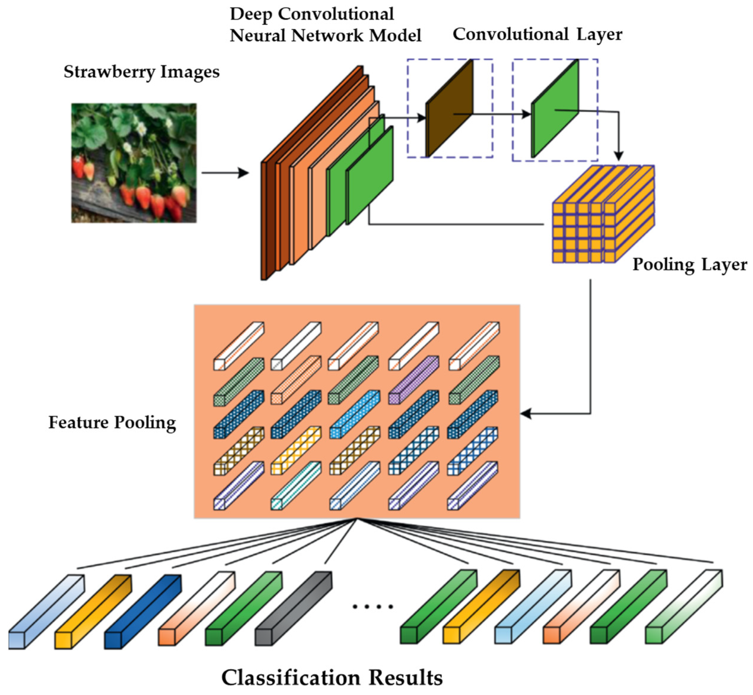
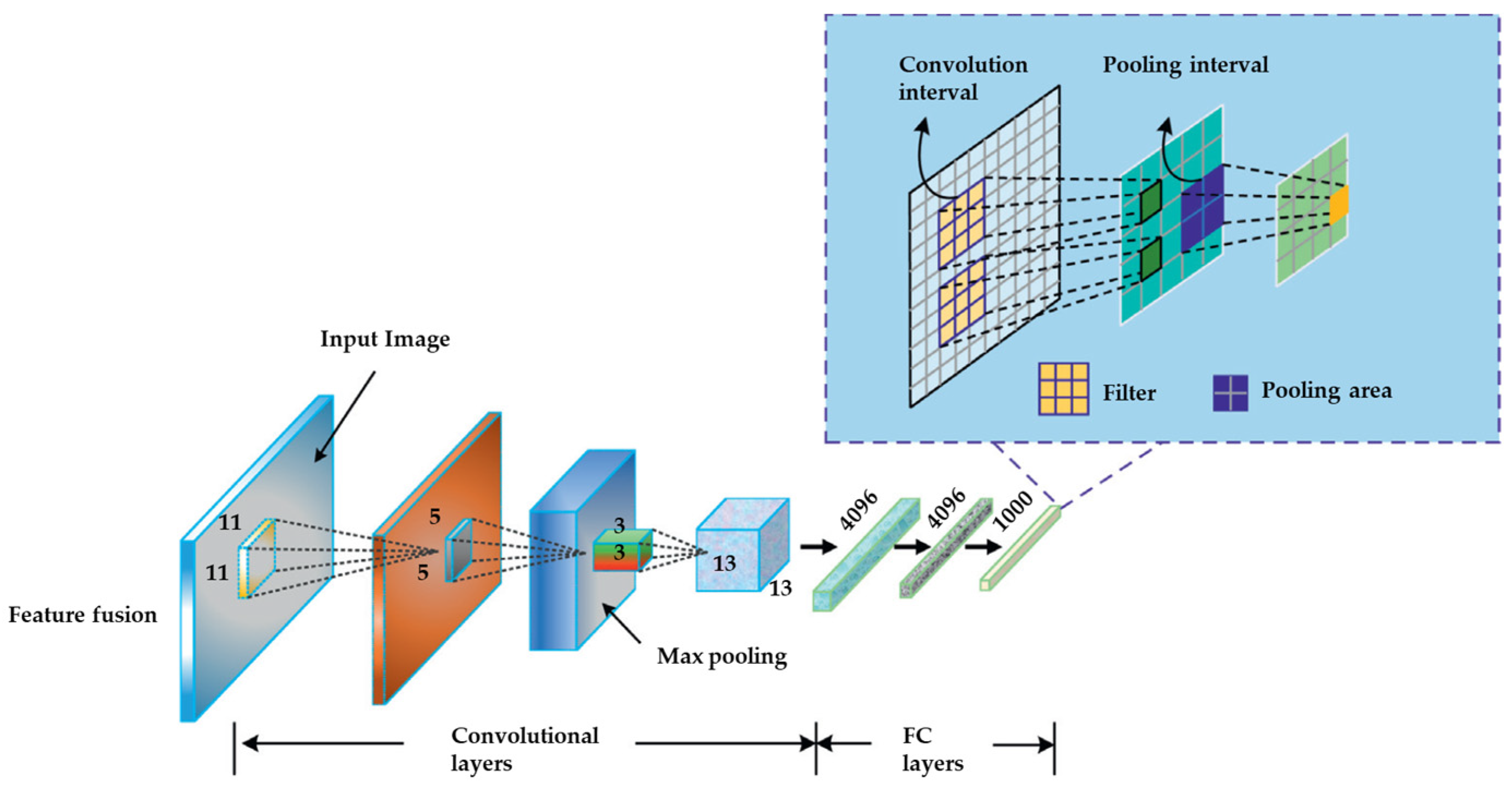
2.1. Convolutional Neural Network (CNN)

CNN is widely recognized as the most prominent and frequently utilized algorithm in the domain of DL. The primary advantage of CNNs over their predecessors lies in their ability to autonomously recognize pertinent features without requiring human oversight. CNNs were developed based on the architecture of neurons in the brains of humans and animals, akin to that of a traditional neural network. To be more precise, within the cat’s brain, a sophisticated arrangement of cells constitutes the visual cortex [25,40,41,42,43].

CNN architecture typically comprises two primary components. The basic architecture of a CNN along with the framework for classification is shown in Figure 1 [44]. The components are illustrated in Figure 2 [44]. The process of feature extraction involves utilizing a convolution tool to isolate and categorize distinct characteristics of an image for analytical purposes. The feature extraction network comprises numerous pairs of convolutional or pooling layers. The fully connected layer employs the output generated by the convolution process to make predictions regarding the image’s class, relying on the feature that was extracted in earlier stages. The objective of this feature extraction CNN model is to decrease the number of features that exist within a given dataset. The process generates novel attributes that encapsulate the pre-existing attributes present in a given feature set. The CNN architecture diagram depicts a multitude of CNN layers (Figure 2).

The input x of a CNN model is structured into three dimensions, namely height, width, and depth. Specifically, the dimensions are denoted as m × m × r, where the height (m) is equivalent to the width. The term “depth” is commonly used interchangeably with “channel number”. As an illustration, in an RGB image, the dimensionality (r) is equivalent to three. The convolutional layer comprises a variety of kernels (filters), represented by the symbol k, each possessing three dimensions (n × n × q), which is analogous to the input image. However, it is imperative that n is smaller than m, while q is either equal to or less than r. Moreover, the kernels serve as the foundation for the regional connections, which possess comparable parameters (namely, bias b^k and weight W^k) to produce k characteristic maps h^k, each with dimensions of (m-n-1). These maps are subsequently convolved with the input, as previously stated. The convolutional layer performs a mathematical operation known as dot product, which involves multiplying its input with the weights, as expressed in Equation (1). Next, by applying the nonlinearity or an activation function to the convolution-layer output, obtain the following [42,43]:

$$h^k=f(W^k\times x+b^k),$$

(1)

After this stage, it is necessary to perform down-sampling on each feature map within the subsampling layers. The aforementioned phenomenon results in a decrease in the network parameters, thereby expediting the training procedure and consequently facilitating the resolution of the overfitting predicament. In the context of feature maps, a pooling function, such as maximum or average, is implemented on a neighboring region of dimensions p × p, where p represents the kernel size. Ultimately, the mid- and low-level features are transmitted to the fully connected (FC) layers, which generate a high-level abstraction akin to the final-stage layers found in a conventional neural network. The scores of classifications are produced by the terminal layer [42,43].

2.1.1. Convolution Layers

The convolution layer is the initial layer that is used to extract numerous image features. This layer performs the mathematical operation of convolution between the input image and a filter of a specific size, M × M. By dragging the filter over the input image, the dot product (M × M) is calculated between the filter and portions of the input image based on the filter’s dimensions. The result is the feature map, which provides information about the image, including its corners and borders. Later, this feature map is transmitted to other layers, so they can learn additional image features. After performing the convolution operation on the input, CNN’s convolution layer passes the result to the next layer. Convolutional layers in CNN are extremely advantageous because they preserve the spatial relationship between pixels [42,43].

2.1.2. Pooling Layers

The pooling layer is a crucial component of convolutional neural networks (CNNs) that aid in identifying the presence and location of features in input images. However, it is important to note that the use of this layer can lead to a reduction in the overall performance of CNNs. This limitation arises from the fact that the pooling layer is primarily concerned with accurately determining the location of features rather than considering their overall significance. The CNN model fails to capture pertinent information [42,43].

The primary function of the pooling layer is to perform subsampling on the feature maps. The generation of these maps is achieved through the implementation of convolutional operations. Stated differently, this methodology involves reducing the dimensions of feature maps of considerable magnitude in order to generate feature maps of smaller sizes. Simultaneously, it preserves the majority of the prominent data (or characteristics) during each phase of the pooling process [42,43]. Similar to the convolutional operation, the pooling operation involves the initial assignment of size to both the stride and the kernel prior to execution. Diverse pooling techniques are at one’s disposal to be employed in different pooling layers. The techniques encompassed in this set comprise tree pooling, gated pooling, average pooling, min pooling, max pooling, global average pooling (GAP), and global max pooling. The most commonly employed pooling techniques are maximum, minimum, and global average pooling [42,43].

2.1.3. Fully Connected Layers

Typically, this layer is situated at the conclusion of every CNN design. In this layer, every neuron is linked to all the neurons of the preceding layer, which is commonly referred to as the fully connected (FC) technique. The neural network architecture comprises synaptic weights and biases, in addition to the interconnected neurons, which facilitate the communication between two distinct layers of the network. Typically, these strata are positioned prior to the output layer and constitute the final layer of a CNN architecture [42,43].

The input image is flattened and subsequently inputted into the FC layer. This process occurs after the preceding layers. Subsequently, the compressed vector is subjected to additional fully connected layers, where mathematical operations are typically performed. At this juncture, the process of classification commences. The rationale behind connecting two layers lies in the fact that the performance of two FC layers surpasses that of a single connected layer. The FC technique in CNN architecture effectively minimizes the need for human supervision [42,43].

This study includes an analysis of two crucial parameters, namely the loss and the activation function, in addition to the three layers previously mentioned. The activation and loss functions are two crucial components in deep learning models that offer significant flexibility and customization options [45,46]. The utilization of functions in problem-solving techniques is comparable to the construction of various sentences through a combination of words. Activation functions are utilized in deep learning tasks to provide neural networks with the capability to express nonlinearity, which enhances the accuracy of the results by enabling better fitting [46,47,48,49,50]. These functions also determine whether information should be transmitted to the next neuron, whereas the loss function is typically utilized to evaluate the precision, resemblance, or adequacy of the predicted output in comparison to the actual value [45,47,48,49,50].

2.1.4. Activation Functions

The fundamental role of activation functions in neural networks of all kinds is to map input values to corresponding output values. The computation of the input value in a neuron involves a weighted summation of the neuron input and its bias, if it exists. The activation function is responsible for determining the firing of a neuron based on a specific input by generating the corresponding output [42,43,47,48,49,50].

In CNN architecture, it is common practice to utilize non-linear activation layers subsequent to all learnable layers, including FC layers and convolutional layers. The non-linear behavior of activation layers in convolutional neural networks (CNNs) results in a non-linear mapping of input to output. This property enables CNNs to learn highly complex features. The capacity to differentiate is a crucial characteristic of the activation function, as it enables the utilization of error back-propagation for network training. The utilization of activation functions is a common practice in CNN and other deep neural networks. The most frequently employed activation functions in these networks are as follows [42,43,47,48,49,50]:

• Sigmoid: This activation function takes real numbers as input and output numbers between zero and one.
• Tanh: It is similar to the sigmoid function in that it accepts real numbers as input, but its output is limited to values between −1 and 1.
• ReLU: In the CNN context, the most widely used function is ReLU. It converts the input’s full values to positive numbers. The key advantage of ReLU over the others is its lower computational load. Occasionally, a few severe difficulties may arise while using ReLU. Consider an error back-propagation algorithm that has a higher gradient running through it. Passing this gradient through the ReLU function will update the weights in such a way that the neuron will never be stimulated again. This is known as the “Dying ReLU” problem. There are some ReLU solutions available to address such difficulties. Instead of ReLU downscaling negative inputs, this activation function ensures they are never ignored. It is used to solve the Dying ReLU issue.
• Noisy ReLU: This function makes ReLU noisy by using a Gaussian distribution.
• Parametric Linear Units: This is similar to Leaky ReLU. The primary distinction is that in this function, the leak factor is updated during the model training process.

2.1.5. Loss Function

The final classification is accomplished by the output layer, which is the final layer of the CNN design. In the CNN model, some loss functions are used in the output layer to determine the expected error created over the training samples. This mistake shows the discrepancy between the actual and projected output. The CNN learning procedure will then be used to optimize it.

The loss function, on the other hand, uses two parameters to determine the error. The first parameter is the CNN estimated output, and the second parameter is the actual output. Diverse loss functions are used in diverse problem categories. Some of the loss function types are explained briefly below [42,43,47,48,49,50].

• Cross-Entropy or Softmax Loss Function: This function is often used to assess the performance of CNN models. It is also known as the log loss function. It returns the probability p ∈ {0,1}. Furthermore, it is commonly used to replace the square error loss function in multi-class classification tasks. It uses softmax activations in the output layer to generate output within a probability distribution.
• Euclidean Loss Function: The Euclidean Loss Function is commonly utilized in regression issues. Furthermore, it is the so-called mean square error.
• Hinge Loss Function: This function is often used in binary classification situations. This issue is related to maximum-margin-based classification. This is especially relevant for SVMs that use the hinge loss function, in which the optimizer strives to maximize the margin around dual objective classes.

2.2. Other Important Variants of CNN

Prior to delving into the next section, it is important to provide an explanation of various CNN variants in order to enhance comprehension of how CNN models generate the desired output based on factors such as data size, complexity, and quality.

2.2.1. AlexNet

The year 2012 marked a significant milestone in the field of computer vision when Alex Krizhevesky and his team introduced a novel CNN model that was deeper and wider than the existing LeNet architecture [33,35,42,51,52]. This new model was put to the test in the ImageNet Large Scale Visual Recognition Challenge (ILSVRC) and emerged victorious, demonstrating its superior ability to recognize visual objects. The AlexNet model demonstrated superior recognition accuracy compared to conventional machine learning and computer vision methods. The discovery marked a notable advancement in the realm of machine learning and computer vision, specifically in the areas of visual recognition and classification tasks. This event also served as a pivotal moment in history, as it sparked a surge of interest in deep learning. The system has the capability to manage several GPUs simultaneously. Subsequent to that year, additional and more complex neural networks, including the notable VGG and GoogleLeNet, were introduced. According to the findings, the official data model exhibits an accuracy rate of 57.1%. Moreover, the top 1–5 results demonstrate an accuracy rate of 80.2%. The performance of conventional machine learning classification algorithms is noteworthy. The AlexNet architecture is a CNN that was specifically developed to process high-resolution RGB images with dimensions of 224 × 224 × 3. The model consists of a total of 62 million trainable parameters [33,35,42,51,52].

2.2.2. Visual Geometry Group (VGG)

VGGNet was a pioneer in investigating how network depth affects CNN performance. The Visual Geometry Group and Google DeepMind, which investigated 16-dimensional architectures, proposed VGGNet [35,53,54,55].

VGG16 increased the network’s size from eight weight layers (AlexNet’s suggested structure) to sixteen weight layers by adding 11 additional convolutional layers. The total number of parameters increased from 61 million to 144 million, but the fully connected layer consumes the majority of them. In ILSVRC2014, the error rate decreased from 29.6 to 25.5 for top-1 val. error (percentage of times the classifier did not provide the correct class with the highest score) and from 10.4 to 8.0 for top-5 val. error (percentage of times the classifier did not include the correct class among its top 5) on the ILSVRC dataset. This suggests that a CNN with a deeper structure can obtain better results than networks with a shallower structure. In addition, they stacked multiple 3 × 3 convolutional layers without an intermediate pooling layer to supplant the convolutional layer with large filter sizes, such as 7 × 7 or 11 × 11. They concluded that this architecture is able to receive the same receptive fields as those with larger filter capacities. Consequently, two stacked 3 × 3 layers are capable of learning features from a 5 × 5 receptive field, albeit with fewer parameters and greater nonlinearity [35,53,54,55].

2.2.3. GoogLeNet

GoogLeNet introduced a network architecture that combines state-of-the-art performance with a lightweight network structure. The concept underpinning an inception network architecture is to keep the network as sparse as possible while taking advantage of the computer’s fast matrix computation capability [15,26,33,53,56,57].

GoogleNet has a much deeper and broader architecture with 22 layers than AlexNet, despite having a significantly smaller number of network parameters (5 million) than AlexNet (60 million). A key component of the GoogleNet architecture is the utilization of the “network in network” architecture in the form of the inception modules. Using parallel 1 × 1, 3 × 3, and 5 × 5 convolutions as well as a parallel max-pooling layer, the inception module can capture a variety of features in parallel. Dimensionality reduction is performed by adding 1 × 1 convolutions before the 3 × 3 and 5 × 5 convolutions (and also after the max-pooling layer) to reduce the quantity of computation required for the implementation to be practical. A filter concatenation layer combines the outputs of these parallel layers. In the version of the GoogleNet architecture that we employ for our experiments, a total of nine inception modules are utilized [15,26,33,53,56,57].

2.2.4. U-Net

U-Net is a typical symmetric encoder-decoder structure. The left half of the encoder is utilized for feature extraction and contains a variety of convolutions and pooling operations. The image is down-sampled, and the correct decoder is used to up-sample, restore the original image’s geometry, and predict each pixel. The encoder and decoder are linked via skip connections in order to incorporate the features of various levels in both the encoder and decoder. U-Net has obtained noteworthy performance on both medical and natural images [29,58,59].

The network has 28 M parameters and is extremely lightweight. Therefore, it has a high potential for use in the segmentation of images of diseased leaves [29,58,59]. In U-Net, an encoder and decoder are connected via a bypass connection. Since the number of convolutional layers in the encoder is comparatively low, the extracted features are at a low level; in contrast, the number of convolutional layers in the decoder is greater, and the corresponding extracted features are at a higher level. There is a substantial semantic difference between the encoder and decoder. Consequently, a semantic disparity may exist between the two combined feature sets, which may have negative effects on the segmentation procedure. UNet only requires a few labelled images for training and has a reasonable training time [29,58,59].

2.2.5. R-CNN

Mask R-CNN is a commonly used reference network in the field of instance segmentation. A novel approach is proposed in this study, wherein a supplementary branch is incorporated into the Faster R-CNN network to facilitate the primary instance segmentation of every detection [14,32,34,60,61,62].

The faster R-CNN network initiates image processing by utilizing a backbone network that exclusively employs convolution layers to extract features from the input image. The generation of detections in Faster R-CNN involves the utilization of a dedicated network known as the Regional Proposal Network (RPN). This network is responsible for processing the features that have been extracted by the backbone. The aim of the research is to determine the likelihood of an object being present and the corresponding offset for each anchor, at every entry position in the RPN. Following the detection phase, a filtering procedure is implemented to identify the most suitable candidates. The elimination of detections beyond the image range and the overlapping of detections are achieved through the utilization of the non-maximum suppression algorithm in this process. The feature regions of the backbone are extracted using final detections. The extracted regions undergo rescaling to a standardized size, achieved through the implementation of RoI-pooling operations in Faster R-CNN and RoI-Align in Mask R-CNN. The input regions are utilized in a neural network to execute a refined adjustment of the initial detection and ascertain its corresponding class. The parallel processing of regions by the neural network in Mask R-CNN is performed concurrently with the primary instance segmentation of detection. The generation of a low-resolution mask from a fixed-size region extracted from the backbone is a characteristic of Mask R-CNN. The methodology employed in this study involves the utilization of a CNN architecture, wherein solely convolutional and transposed convolutional operations are performed. A mask is generated for each class upon detection. Following the classification of detections by the neural network, a mask corresponding to its respective class is allocated to each detection [14,32,34,42,60,61,62].

2.2.6. YOLO

The YOLO algorithm, an abbreviation for “You Only Look Once,” is a one-shot detector that falls under the category of object detection algorithms. The network under consideration is characterized by its impressive processing speed. However, the accuracy of the outcomes may be slightly reduced as a result of the image being passed through the network only once. The implementation of this network architecture can prove to be highly beneficial as a foundation for software systems that involve real-time operations and require the ability to process a significant number of frames [4,40,42,43,61,63].

The utilization of a fixed-size grid that overlays the input image and partitions it into multiple cells is a crucial characteristic of YOLO-based networks. In this study, each cell is assigned an array of predicted values, including x and y coordinates representing the upper left and lower right points of the bounding box or the coordinates of the bounding box center. Additionally, the array includes w and h values indicating the width and height of the bounding box, as well as C, which represents the probability of the detected object belonging to a specific class within the image. The division of the input image into S cells is a crucial step in the neural network’s processing pipeline. This approach enables the network to analyze the image at a more granular level, allowing for more accurate feature extraction and classification. By segmenting the image into smaller units, the network can identify patterns and relationships between adjacent cells, leading to improved performance in tasks such as object detection and image recognition. Each object depicted in the image is associated with a specific cell that is responsible for its prediction. The location of the object’s center within the grid determines this cell. The research involves performing predictions for B bounding boxes and C probabilistic estimates of classes for each cell. The resulting tensor from the terminal output is an S × S × (B × 5 + C)-dimensional tensor [4,40,42,43,61,63].

Upon receiving the input image, the network conducts the requisite procedures to partition it into individual cells. The non-max suppression algorithm is applied in order to eliminate unnecessary predictions during the process.

The following is a list of the elements that make up the dataset that the algorithm uses: This study examines the impact of bounding box values, object probability, and overlap thresholds on the detection of desired objects in images. The output data displays a list of predictions that have undergone a filtering process consisting of a series of specific actions. Initially, an empty list is created and subsequently populated with the prediction that has the highest probability of the object’s presence in the image. Subsequently, the Intersection Over Union (IOU) values are computed for this prediction and all other predictions. When the IOU (Intersection Over Union) values surpass the predetermined overlap threshold, the corresponding anticipated bounding box is eliminated. The final output of the last convolutional layer yields the frame coordinates, including the center coordinates along with the width and height [4,40,42,43,61,63]. The latest version available from the YOLO family is the YOLO V7.

2.2.7. ResNet

The ResNet architecture is a comprehensive neural network that is constructed through the iterative incorporation of residual learning modules. He et al. (2016 [64]) proposed the ResNet model as part of their research at the Microsoft Research Institute. The ResNet model has been found to exhibit high accuracy in various applications and has been observed to possess a high degree of compatibility with other network structures, making it a promising candidate for integration into complex network architectures [8,15,41,53,57,65,66,67,68]. The ResNet architecture incorporates a direct link, also referred to as a highway network, to enable the original input information to be transmitted directly to the subsequent layer. Residual modules have been introduced to address the issue of gradient dispersion and improve the feature learning capacity and recognition accuracy. The input variable x was subjected to convolution with W₁ and W₂ to produce the output variable f (x, W₁, W₂). The ReLU activation function was utilized in the residual module unit, resulting in the final output y being represented by the following Equation (2) [15,57,65,66].

$$y=f\left(x,W_1,W_2\right)+W_{s}x$$

(2)

The weighting parameters W₁ and W₂ are to be learned, while Ws is a square matrix that transforms the input residual module dimension to the output dimension represented by x. The ResNet network structure employs two types of residual modules. The first type consists of two consecutive 3 × 3 convolution networks, while the second type consists of three convolution networks with sizes of 1 × 1, 3 × 3, and 1 × 1. The ResNet architecture is designed to allow for flexibility in the number of network layers, with popular configurations including 50, 101, and 152 layers. These layers are constructed using residual modules, as previously described [15,57,65,66]. ResNet50 is a well-known network architecture consisting of 50 layers.

3. Applications of Deep Learning in Strawberry Farming

3.1. Strawberry Disease Detection

3.1.1. Multiple Disease Detection

Disease issues are primarily responsible for the decline in vegetable quality and productivity, which results in economic losses for producers, and have a close relationship with daily economic activities [4,56,65]. As one of the most important commodities grown in greenhouses, strawberries also face numerous disease issues. The ability to detect and identify the strawberry diseases with rapid manner and take the corresponding control measures is important for ensuring strawberry growth, curing the disease, and increasing farmers’ income. Although different diseases exhibit some symptoms in the visible light spectrum, the information on their symptoms is complex and subject to change, and only plant specialists with specialized training can identify and diagnose these diseases. With the advancement of computer vision, there are a variety of methods for resolving plant detection issues since infection spots are initially observed as blotches and patterns on leaf surfaces. Several techniques for precisely detecting and classifying plant infections have been proposed by researchers [4,9,28,32,56,65,66,69,70,71].

Many investigations developed DL models to identify multiple diseases as the output of different classes. We have referred to multiple disease detection as multiple classes.

Table 1. Summary of common diseases that occurred in strawberries and some of its fundamental characteristics.

Common Strawberry Diseases	Description
Bacterial wilt	This disease, also referred to as strawberry leaf blight, is distinguished by dry, brown necrotic leaf patches and huge brown V-shaped lesions along the leaf margin, midrib, and major veins, which are caused by Pseudomonas solanacearum.
Verticillium wilt	It is caused by Verticillium dahliae (Kleb.), a soil-borne plant fungus that can lay dormant in the soil for years until it recognizes the presence of a healthy strawberry plant less than 2 mm away. When this happens, the fungus produces lengthy hyphae that feed on the plant.
Leaf spot	The disease, known as Mycospherella leaf spot, is caused by the fungus Mycosphaerella fragariae and is one of the most common illnesses in strawberries. The fungi mostly damage the leaflets, causing them to turn purple, which eventually turns brown.
Angular leaf spot	The disease, commonly known as bacterium stain, is caused by the bacteria Xanthomonas fragaria. The term is obtained by the appearance of pale green dots that grow until they are visible on the sheet.
Anthracnose fruit rot	It is a rot produced by Colletotrichum fragariae, Colletotrichum acutatum, and Colletotrichum gloeoporioides. When the plant is subjected to high temperatures and humidity, rot develops.
Blossom blight	It caused by Pseudomonas marginalis and disease symptoms began with gray sporulation of the fungus on the stigmas and anthers of strawberry flowers, followed by necrosis and complete flower abortion
Snake eye	It is a widespread disease caused by microclimate changes, such as night temperature increase and a wet environment, that can damage strawberries at any stage of development. Infections are recognized by the appearance of small, deep purple/brown, spots shaped like round snake eyes on the plant’s upper leaf surface.
Gray mold	Caused by the Botrytis cinerea Pers. F. fungi or simply Botrytis. The name gray mold is given due to the appearance of gray-colored mold formed on the leaf and calyx, which may affect the fruit.
Powdery mildew leaf	Caused by the Sphaerotheca macularis fungi. Powdery mildew is caused when the plantation is submitted to a dry and hot climate. It manifests as the apparition of whitish spots on the inferior face of the leaf. It also affects the fruits and can be observed by the fruit’s discoloration and spots.
Powdery mildew	It is caused by Sphaerotheca macularis fungi, affects the fruits, and can be observed by the fruit’s discoloration and spots.
Botrytis rot	Botrytis rot or fruit rot is caused by Botrytis cinerea Pers. F. fungi or simply Botrytis. It can infect strawberry flowers when spores land on them and are exposed to free water during cool weather. Infections can either cause flowers to rot or Botrytis can become dormant in floral tissues.

contains a description of the prevalent diseases and their fundamental characteristics, whereas, the application of deep learning algorithms used for strawberry farming from the reviewed studies was summarized in Table 2. The framework for disease identification were shown in Figure 3. On the other hand, several researchers have devised models to predict the early occurrence of specific plant diseases. Several researchers used CNN to detect multiple diseases (classes) in strawberries; as a result, they created a variety of single models capable of detecting multiple diseases. For instance, the previous study [72,73] developed AlexNet, DenseNet-169, Inception v3, ResNet-34, SqueezeNet-1.1, and VGG13 to detect 38 classes of diseases, or healthy plants for 14 crop species using AlexNet, DenseNet-169, Inception v3, ResNet-34, and SqueezeNet-1.1. Eight training configurations (six CNN architectures, three strategies) employ the same hyperparameter values (momentum = 0.90, weight decay = 0.00005, learning rate = 0.001, and batch sizes = 20). This evaluation utilized the PlantVillage datasets. The dataset included 54,323 images. A background class consisting of 715 images was used to train the classifier to distinguish between plant leaves and the environment. The background class was constructed using a set of color images from a public dataset made available by Stanford. The integrated dataset containing the background class contains 39 classes and consists of 55,038 records. The following cutting-edge architectures were utilized: The accuracy obtained by training from scratch with an 80–20 train-test distribution includes AlexNet, which achieved 97.82% accuracy, and GoogleNet, which achieved 98.35% accuracy. In contrast, transfer learning training produced the following results: AlexNet with 99.24% accuracy and GoogleNet with 99.34% accuracy. Using transfer learning, Inception v3 attained the highest accuracy, i.e., 99.72%. Among the classes of diseases covered, only one class of fungal leaf diseases of strawberry plants was covered, namely leaf scald. The developed model did not account for the other classes of strawberry leaf diseases (leaf blight and leaf spot), rendering it incapable of differentiating between the three classes of these diseases. For a better understanding, results of a previous study are shown in Figure 4.

Similarly, Brahimi et al. (2018) [33] conducted a study in which a CNN-based method for leaf disease grade identification was proposed. As experimental data, 18,347 leaf images were selected from PlantVillage, including 10 classes of leaf diseases from eight crop species. Initially, a nonuniform illumination image was processed using an adaptive adjustment algorithm based on a two-dimensional (2-D) gamma function. The segmentation of diseased leaf images using a threshold segmentation method yielded binary images. The ratio of the number of pixels in the lesion area to the number of pixels in the diseased leaf area was determined, and this ratio served as the classification threshold for disease grades. Therefore, it was used to ascertain the severity category of the disease. In addition, a ResNet50-based CNN was proposed to classify disease severity, with an accuracy of 95.61 percent. Among the 10 featured classes of plant diseases, this study also considered strawberry leaf scorch, a singular class of strawberry plant fungal leaf diseases.

Likewise, several studies [4,9,28,32,56,65,66,69,70,71] have developed models to detect the strawberry leaf disease along with the other plants since they have utilized standard data sets such as Plant Village and Kaggle. Thus, they detected the fungus-infected leaf of strawberries as another plant disease. Cheng Dong et al. (2021) [72] developed a model for the automatic recognition of strawberry diseases that is particular for the strawberry plants. In that study, he fine-tuned an AlexNet model named improved AlexNet, and they compared the detection results with Resnet50, MobileNet_v2, and SCNet-50. In the end, that study developed a successful model with 97.35% prediction accuracy, less training time (363.6 s), and minimum model size (14.1 MB). Similarly, research on strawberry disease diagnosis based on an improved residual network recognition model was developed by Wenchao and Zhi, 2022 [8]. As in the previous study, this study improvises an original ResNet50 named G-ResNet50 and achieved a precision of 99.5% and F1 98.4. They utilized the Agricultural Diseases and Pests (IDADP) dataset from Plantvillage. Also, they compared the model’s performance with InceptionV3, ResNet50, MobileNetV2, and VGG16. From their results, compared to the other four network models, the G-ResNet50 has a faster convergence speed and higher generalization ability. The G-ResNet50 can perform deep training, which can alleviate the problem of performance degradation as the number of layers increases. The average recognition accuracy rate of the G-ResNet50 reached 98.67%, and the false recognition rate is lower than the other four networks.

Another study by Kim et al. (2021) [74] detected strawberry fungal leaf disease using a deep normalized neural network. The disease classes include strawberry leaf spot, leaf scorch, leaf blight, and a class where two diseases (leaf blight and leaf scorch) occur together. They achieved a classification accuracy of 98%, precision of 97%, recall of 95.7%, and F1-score of 96.3%. In a separate study [29], UNet architecture was used to determine the extent of fungal diseases influencing plant leaves. In this investigation, more than fifty varieties of strawberry leaf were investigated. Using the UNet architecture, feature extraction based on the color, texture, and geometry of the cluster and the classification of the classes were completed. This study finally obtained a prediction accuracy of 95%. Similarly, another study [71] utilized GoogLeNet, Resnet50, and VGG-16 models to identify strawberry diseases. This research utilized two kinds of input datasets from PlantVillage. They also evaluate the variations in model performance based on the number of epochs. They attained a classification accuracy rate of 100 percent for leaf blight cases affecting the crown, leaf, and fruit; 98 percent for gray mold cases; and 98% for powdery mildew cases. In 20 epochs, an accuracy rate of 99.60% was obtained from the feature image dataset, which was greater than the accuracy rate of 1.53% from the original dataset.

Similarly, the authors of a previous study [75] utilized PlantNet to detect strawberry diseases. They incorporated PlantNet and a two-stage cascade disease detection model as the foundation of the architecture. For the LifeCLEF 2017 challenge, PlantNet has been pre-trained on plant data using the PlantCLEF dataset. The results indicate that the cascade detector combined with PlantNet increased precision by up to 5.25 percent mAP. A single-stage detector with PlantNet achieved 86.4% mAP on the challenging task of strawberry disease detection, representing a 3.27% advance over a model pre-trained on the ImageNet dataset. In addition, the cascade model generated approximately 91.65% mAP, representing a 5.25% improvement over a model without cascades. The primary advantage of this model is that it is capable of overcoming a lack of annotated data by employing plant domain knowledge, and that the human-like cascade detection strategy is effective at enhancing accuracy. Moreover, in a previous study [74], a CNN with deep normalization was used to detect disease. The authors created a CNN model with the activations of the intermediate layers normalized. This claim asserts that this technique increases model precision and accelerates training. Comparing VGG 16, GoogleNet, and ResNet 50, they identified the following classes: Strawberry Healthy, Leaf Scorch, Strawberry Leaf Blight, Strawberry Leaf Spot, Strawberry Leaf Blight, and Leaf Scorch. In a dataset containing 1134 images, this study obtained an overall accuracy of 98% for all classes considered and an accuracy of 86.67% for the simultaneous occurrence of leaf blight and leaf scorch.

Figure 4. Samples of the final disease detected results obtained in a previous study in which blue rectangles represent the merged suspicious areas of disease, and the red boxes are the diseases detected in the second stage [75].

Figure 4. Samples of the final disease detected results obtained in a previous study in which blue rectangles represent the merged suspicious areas of disease, and the red boxes are the diseases detected in the second stage [75].

Furthermore, a CNN model based on deep metric learning is developed to classify known and unknown diseases in strawberry leaf samples (Hu et al. (2023)) [76]. The KNN classifier is used as the final classification layer for diseases with known and unknown samples. For accurate object detection, FPN-Based Faster R-CNN was utilized in this study. Still, the ResNet50 network was utilized along with DML-embedded features with margin triplet and cross-entropy losses. It could be utilized as a Region of Interest (ROI) classifier because the DML-based K-NN classifier has a high recall and precision for both known and unknown diseases and an accuracy of 97.8%. Using actual field data, the proposed method obtains a high mAP of 93.7% for detecting known strawberry disease classes.

Recent research, Zhang et al. (2022) [77] developed a class-attention-based lesion proposal CNN for the identification of strawberry disease. The CALP-CNN models locate the principal lesion object from the complex background using a class object location module (COLM) and then apply a lesion part proposal module (LPPM) to suggest the discriminative lesion details. The CALP-CNN can simultaneously resolve interference from the complex background and misclassification of similar diseases due to its cascade architecture. In this investigation, the model was fed the Strawberry Common Disease Dataset (SCDD), which contains 11 common strawberry disease datasets. The classification results of CALP-CNN are 92.56% accuracy, 92.55% precision, 91.80% recall, and 91.96 percent F1-score. The CALP-CNN outperforms six other algorithms by 6.52% (on F1-score).

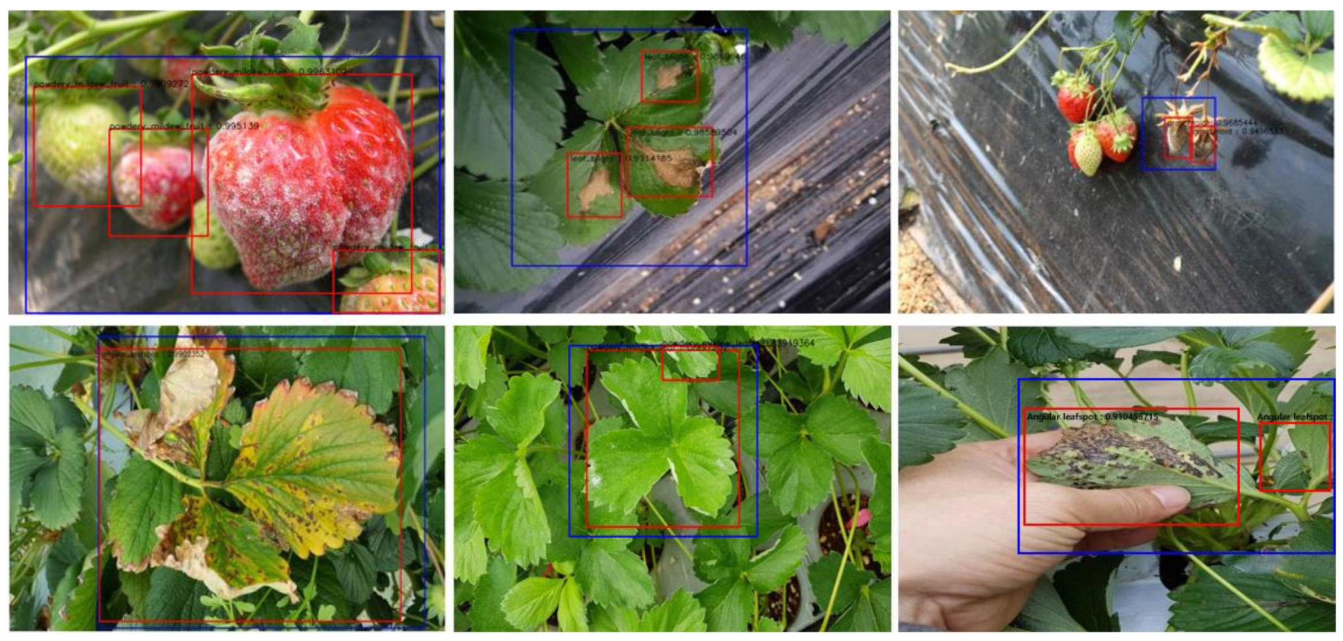
3.1.2. Particular Disease Detection

Verticillium wilt detection: Sometimes emphasizing a single approach to solving a problem will result in more trustworthy solutions and an in-depth understanding of the specific situation [67,78]. Accordingly, a prior study [31] based on multi-task learning and attention networks was created to identify Verticillium wilt in strawberries. This paper proposes a method for detecting and identifying Verticillium wilt in strawberry photos. It is based on Faster R-CNN and multitasking. In SVWDN, the identified components are used to assess whether the entire plant is affected by verticillium wilt, in addition to identifying and categorizing the petioles and young leaves in the photos. A new dataset of verticillium wilt in strawberries was created. It consists of 3531 images taken from a strawberry greenhouse, of which 2742 are verticillium wilt samples and 789 are healthy samples. The dataset is divided into 4 categories: healthy_leaf, healthy_petiole, verticillium_leaf, and verticillium_petiole. Each of the images also includes a label stating whether the strawberry has Verticillium wilt. A novel disease detection task that determines whether the plant has Verticillium wilt based on the discovered young leaves and petioles was added to multi-task learning. They captured images from various perspectives throughout the data collection to increase sample diversity. They create the channel-wise attention weight vector for the high-level feature maps using the multi-level features. The network with attention performs object detection better than the disease detection network (DDN), and on the collected dataset, the accuracy of the illness detection task is 99.95%. According to the findings, they were able to detect objects in four categories with an accuracy of 99.95% and strawberry Verticillium wilt with an mAP of 77.54%.

Powdery mildew disease diagnosis: An earlier study [56] developed a powdery mildew disease diagnosis method on strawberry leaves utilizing RGB images based on DL. The models optimized AlexNet, SqueezeNet, GoogLeNet, ResNet-50, SqueezeNet-MOD1, and SqueezeNet-MOD2 and were all comprehensively evaluated. To avoid overfitting and consider the different shapes and directions of the leaves in the field, they also employed augmented data that was gathered from 1450 photos of healthy and sick plants. The six DL algorithms utilized in this study had an overall average classification accuracy (CA) of >92%. ResNet-50 distinguished between healthy and infected leaves with a CA of 98.11%; however, when computation time was considered, AlexNet processed 2320 pictures with a CA of 95.59% in just 40.73 s. With a CA of 92.61%, SqueezeNet-MOD2 would be suggested for PM detection on strawberry leaves while considering the memory needs for hardware deployment. ResNet-50 had a statistically larger CA (98.11%) than the other algorithms, although there was no discernible difference in the other methods’ CA. SqueezeNet-MOD2 had the least demanding criteria for possible hardware memory. ResNet-50 took the longest to process 2320 photos, taking 178.20 s, while AlexNet took the shortest, taking 40.73 s. The CNN algorithms tested took considerably different amounts of time, with AlexNet and SqueezeNet-MOD2 taking the least amount of time.

Gray mold disease detection: Recently, a study was conducted using deep learning networks to detect gray mold disease and its severity on strawberries [28]. Due to the absence of entirely connected layers, UNet has fewer network parameters, allowing the network to train effectively with fewer training datasets. Three isolated strawberry plant groups were inoculated with three distinct doses of the pathogen (Botrytis cinerea). Using an RGB camera in the field, the development of visible symptoms and their progression on the leaf were recorded non-invasively. A total of 400 leaf images with corresponding annotation images were divided by a ratio of 80% to 20% into training and testing sets. Thus, 320 images were utilized for training and validation, while 80 were utilized for assessment. Using fivefold cross-validation datasets, the model was then trained and verified. The results were evaluated using the VGG16-XGBoost classifier, the K-means algorithm, and the Otsu method. They noted that Unet outperforms the competition with an accuracy rate of 82.12%, less memory consumption (~22 MB), and quick testing results (within 0.2 s for an image on a standard computer). They noted that the implementation of the pre-trained VGG16 initial two convolutional layers enabled the XGBoost classifier to achieve an acceptable level of performance. According to this study, the performance of the UNet model was superior because the feature maps generated on the encoder side are concatenated with the feature maps generated on the decoder side, thereby increasing the accuracy of pixel segmentation. Additionally, the deeper layers with numerous filters enable the network to recognize minute image details, thereby enhancing its segmentation performance. In contrast, the decoder sectioned up and converted the reduced image size to its original size, resulting in the same size for input and output images, making it simple to calculate the severity of the disease.

3.2. Strawberry Fruit Detection

The assessment of plant growth is a fundamental methodology for ensuring an optimal agricultural yield in terms of both quality and quantity [34,62]. Currently, two types of protocols are followed when using these systems: (1) A person must manually go around a greenhouse and take pictures of the suspected areas using a handheld camera. (2) Next, the images are processed using automatic detection systems. Robotic systems are utilized for conducting surveillance activities within the greenhouse environment and capturing necessary images in an autonomous manner. These images are then subjected to processing by an automated disease detection system.

In a prior study, Yu et al. (2019) [62] proposed a method for detecting strawberry fruit targets using Mask R-CNN. In an unstructured environment, Mask R-CNN not only accurately recognized the categories (ripe or unripe fruit) and marked out object regions with bounding boxes but also extracted object regions from the background at the pixel level. Moreover, the identification of strawberry picking locations can be accomplished through an analysis of the shape and edge characteristics of the mask images produced by Mask R-CNN. They used ResNet50 as a backbone network, while features such as multi-scale fusion features (color, shape, texture, geometry, etc.) were extracted using ResNet50/101 + FPN. Finally, Mask R-CNN is used as a target detection model. Before the training for the strawberry identification, the model was pre-trained using COCO datasets using transfer learning to solve the problem of a small training set COCO as it is a huge dataset for object detection and image segmentation, with 328 k images in 91 categories. The pre-training model extracted the general features of all categories from COCO. The study successfully developed a Mask R-CNN model capable of autonomously detecting mature and immature strawberries, with the model generating mask images of the fruit as output. The fruit detection results of 100 testing images showed that the average detection precision, recall, and MIoU rates were 95.78%, 95.41%, and 89.85%, respectively.

In order to predict mature and immature greenhouse-grown strawberries, Pérez-Borrero et al. (2020) [79] conducted a thorough evaluation of R-CNN models in 2018. The authors assess the performance of R-CNN through an analysis of its training behavior, classification accuracy, localization accuracy, and errors during detection. Initially, a set of 421 images was manually captured using a camera. Subsequently, a uniform removal of 48 images was performed from this set. The experiment utilized a total of 373 images, from which 551 mature and 923 immature fruits were identified and included for analysis. Images are removed in cases where the resolution of the fruit is low due to issues such as poor lighting or a lack of focus by the camera. The selection of the desired dataset is based on the threshold of fruit color. As a result, the pink-colored strawberry marking was excluded during the prepossessing stage due to the possibility that pink fruits may not have undergone sufficient exposure to sunlight to facilitate the development of anthocyanin pigments. In the process of training preparation, the bounding boxes were utilized to accurately enclose the outer region of the fruits. Furthermore, an object is chosen if the occlusion is minimal. The researchers assessed the outcomes by utilizing two parameters, namely average precision (AP) and bounding box overlap (BBOL). The former parameter is a composite measure of detection success and confidence in detection, while the latter parameter quantifies the accuracy of localization. The created deep learning model attained an AP of 88.03% and 77.21%, and a BBOL of 0.7394 and 0.7045, respectively, for the mature and immature categories.

A recent study conducted by [80] proposes a novel instance segmentation approach for strawberries utilizing Mask R CNN, with the aim of enhancing the harvest robot’s capacity to identify ripe strawberries. The present study has acquired a novel data set comprising 3100 strawberry images with high resolution, accompanied by manually segmented ground-truth images. Most of the researchers used the bounding box method for data annotations. They made the annotations using an interactive polygon tool developed in MATLAB that defines the continuous or discontinuous contour of the strawberry by using a sequence of points. The strawberries are classified into three categories based on their pixel size in the captured image: small (area ≤ 32 Pixel), medium (32 Pixel < area ≤ 96 Pixel), and large (>96 Pixel). Moreover, that study introduces a new metric called Instance Intersection Over Union (mI²oU), which works on a labelled image, where each pixel only belongs to an instance. The paper attains the following AP values: 45.36 for mean AP, 07.35 for AP small, 50.03 for AP medium, and 78.30 for AP big. The mean mI²oU, mI²oU small, mI²oU medium, and mI²oU big values obtained were 87.70, 39.47, 77.10, and 90.12, respectively. In that study, the process of filtering and grouping candidate regions effectively replaced the object classifier and bounding box regressor.

A recent scholarly investigation [81] utilized hyperspectral imaging technology in conjunction with CNN models to assess the degree of ripeness of strawberries in a field setting. The study utilized hyperspectral imaging (HSI) systems, which combine traditional imaging and spectroscopy methods to simultaneously gather spatial and spectral data. This information was then utilized to classify both early ripe and ripe strawberry samples. The study in question opted to utilize specific wavelengths as input for their CNN models, drawn from both fields (530 and 604 nm) and laboratory (528 and 715 nm) datasets. The HSI technology employed in the study is capable of covering a broad range of wavelengths spanning from 370 to 1015 nm. The selection of these spectral feature wavelengths was made with care and consideration. The application of Principal Component Analysis (PCA) was employed to identify the salient features among the extracted features. Furthermore, the SVM algorithm was employed as the ultimate classifier, while a fine-tuned pre-existing AlexNet was utilized as the foundational architecture of the model. The study achieved a 98.6% accuracy rate for the infield test dataset, while the laboratory test dataset was anticipated to have a perfect accuracy rate of 100%.

Table 2. Summary of application of deep learning algorithms used for strawberry farming from the reviewed studies.

Category	Parameters	Used Tools and Techniques	Reference
Disease detection	Multiple classes	AlexNet	[72,73]
		Improved ResNet50	[8]
		DCNN	[44]
		AlexNet, DenseNet-169, Inception v3, ResNet-34, SqueezeNet-1.1 and VGG13	[33]
		Class-attention-based lesion proposal convolutional neural network	[77]
		GoogLeNet model, Resnet50, and VGG 16	[71]
		DNN (PlantNet)	[75]
		YOLO	[4]
		CNN (a location network, a feedback network, and a classification network)	[82]
		Mask R-CNN	[9]
		CNN	[83]
		AlexNet and GoogLeNet	[84]
		YOLO	[27]
	Fungal leaf disease	Multi-directional Attention Mechanism—Dual Channel Residual Network	[85]
		DCNN	[86]
		DCNN	[53]
		UNet	[29]
		CNN, VGG 16, GoogleNet, and Resnet 50	[74]
	Gray mold disease	UNet	[28]
	Verticillium Wilt	Faster R-CNN and multi-task learning	[31]
	Powdery mildew disease detection (Leaf)	AlexNet, SqueezeNet, GoogLeNet, ResNet-50, SqueezeNet-MOD1, and SqueezeNet-MOD2.	[56]
	Known and unknown diseases	Deep Metric Learning-Based KNN Classifier	[76]
Fruit detection	Ripe or unripe fruit	Mask-RCNN	[62]
		AlexNet	[81]
		R-CNN	[79]
		Mask R-CNN	[80]
	Species detection	CNN	[37]
Fruit quality	Plumpness assessment	Faster-RCNN	[34]
	External quality of fruits	CNN	[11]
		AlexNet, MobileNet, GoogLeNet, VGGNet, and Xception, and Two layers CNN architecture	[35]
Wellbeing	Leaf wetness detection	CNN	[87]
Yield	Yield detection	Faster-RCNN	[14]

Table 2. Summary of application of deep learning algorithms used for strawberry farming from the reviewed studies.

Category	Parameters	Used Tools and Techniques	Reference
Disease detection	Multiple classes	AlexNet	[72,73]
		Improved ResNet50	[8]
		DCNN	[44]
		AlexNet, DenseNet-169, Inception v3, ResNet-34, SqueezeNet-1.1 and VGG13	[33]
		Class-attention-based lesion proposal convolutional neural network	[77]
		GoogLeNet model, Resnet50, and VGG 16	[71]
		DNN (PlantNet)	[75]
		YOLO	[4]
		CNN (a location network, a feedback network, and a classification network)	[82]
		Mask R-CNN	[9]
		CNN	[83]
		AlexNet and GoogLeNet	[84]
		YOLO	[27]
	Fungal leaf disease	Multi-directional Attention Mechanism—Dual Channel Residual Network	[85]
		DCNN	[86]
		DCNN	[53]
		UNet	[29]
		CNN, VGG 16, GoogleNet, and Resnet 50	[74]
	Gray mold disease	UNet	[28]
	Verticillium Wilt	Faster R-CNN and multi-task learning	[31]
	Powdery mildew disease detection (Leaf)	AlexNet, SqueezeNet, GoogLeNet, ResNet-50, SqueezeNet-MOD1, and SqueezeNet-MOD2.	[56]
	Known and unknown diseases	Deep Metric Learning-Based KNN Classifier	[76]
Fruit detection	Ripe or unripe fruit	Mask-RCNN	[62]
		AlexNet	[81]
		R-CNN	[79]
		Mask R-CNN	[80]
	Species detection	CNN	[37]
Fruit quality	Plumpness assessment	Faster-RCNN	[34]
	External quality of fruits	CNN	[11]
		AlexNet, MobileNet, GoogLeNet, VGGNet, and Xception, and Two layers CNN architecture	[35]
Wellbeing	Leaf wetness detection	CNN	[87]
Yield	Yield detection	Faster-RCNN	[14]

3.3. Strawberry Fruit Type Detection

In general, deformed products influences quality, which is the primary variable in terms of economics. Nubbins and button berries are the most common names for malformed berries, which are caused by common external destructive agents [3,88]. Strawberries will develop deformities due to cold injury (specifically frost damage to the pistillate portion of the flower) and nutrient deficiencies (specifically a lack of calcium or boron). In addition, they distinguished between oblate, globose, globose conic, conic, long conic, necked, wedge, long wedge, and short wedge based on the morphology of the strawberry [3,37,88]. Fruits with conic and wedge configurations are the most frequently consumed by humans. In a previous study [37], the shape-based classification of strawberries was examined. For this investigation, a Kaggle dataset containing 8554 images was utilized. The authors used 4488 images for training, 1928 images for validation, and 2138 for testing, all belonging to 13 species of strawberries. In addition, they use eight varieties of strawberries (as previously stated) to identify the wedge and conic shapes. In addition, they developed a fundamental CNN structure with four convolutional layers, each with a Relu activation function and a max pooling layer. The same network was used to extract pixel size and other physical observations from full-color images, among other features. Intriguingly, this study’s detection rate was 100%, whereas the training result was 99.99%. However, this study does not compare the results to those of other models to demonstrate the model’s validity. Despite the fact that fruit morphology and deformed fruits are significant scenarios, few studies have been conducted to detect them.

3.4. Strawberry Fruit Quality Detection

Color and shape identification: The utility of automatic fruit grade classification lies in its ability to sort harvest production according to fruit quality. The utilization of a grading classification system can serve as a valuable tool in various aspects of the agricultural industry. It can aid in the determination of pricing, ensure the fulfillment of orders that meet specific quality standards, and facilitate post-harvest processing procedures. A previous study [35] was conducted that involved the creation of a basic CNN model featuring two convolutional layers, which was used as the standard network for the study. The authors evaluated and compared five commonly used CNN architectures, namely AlexNet, GoogLeNet, VGGNet, Xception, and MobileNet, for prediction purposes. Furthermore, the complexity of various architectures is assessed by comparing the training time and the resulting model size after training. A total of 1870 RGB images of fruit were gathered for the study, utilizing two digital cameras and three smartphone cameras to capture images at varying resolutions. The images were initially categorized into two distinct classes: the bad and good classes. The classification of strawberries into good and bad categories is based on their ripeness, condition, and quality. Those that are overripe, damaged, or rotten are considered bad, while the remaining ones are classified as good. The data were grouped into four class labels: a good class with three ranks (first, second, and third rank) and a bad strawberry class (fourth rank). In this study, strawberries were evaluated and categorized into three ranks based on their physical characteristics. The first rank consisted of strawberries with a light red color and normal shape, while the second rank included strawberries with a dark red color and normal shape. The third rank comprised strawberries with an abnormal shape but was still considered to be of good quality. The dataset analyzed in this study comprises a total of 1870 images, which were categorized into two groups based on their quality. The first group consisted of 1000 images that are good quality, with 523 images classified as first rank, 355 images as second rank, and 122 images as third rank. The second group comprised 870 images that were classified as bad quality, all of which were ranked as fourth rank. VGGNet exhibited superior performance relative to all other architectures in the realm of architecture comparison. Specifically, VGGNet achieved a 96.49% accuracy rate in the context of a two-class classification and an 89.12% accuracy rate in the context of a four-class classification. In contrast to other models, VGGNet’s deep training process (13 layered networks) resulted in larger model size and longer training time. On the other hand, GoogLeNet exhibited strong performance (91.93% accuracy on two-class classification and 85.26% accuracy on four-class classification) while requiring less space (0.6 MB) and a shorter training time (853.29 s). Some of the references for the spatial features used to detect the strawberries is shown in Figure 5.

Freshness detection: Non-climacteric fruits like strawberries are prone to rapid metabolic changes, contamination, cellular damage, softening, and discoloration after harvest, during distribution, and during storage processes. These factors can lead to deterioration in appearance. Preserving the freshness of strawberries is a complex process compared to other horticultural fruits [11]. This is due to their susceptibility to mold development and the loss of characteristic flavors. The high cost of transporting strawberries over long distances is a consequence of the current situation. Automated and rapid monitoring systems are necessary for screening large quantities of products. In a prior investigation [11], DL was employed to evaluate the external quality of strawberries. The strawberries procured from the store were subjected to storage at a temperature of 25 °C. The strawberries were categorized into three groups based on their condition: fresh strawberry (FS), bruised strawberry (BS), or moldy strawberry (MS). In this study, the abbreviation FS is used to represent strawberries at the beginning of the storage period, which was referred to as day 0. The observed phenomenon, denoted as BS, refers to the partial surface deterioration of strawberries during the first two days. The presence of surface mold on strawberries was observed on the second and third days, as indicated by the abbreviation MS. The methodology employed in this study involved establishing specific criteria for each state. The selection of FS was based on the absence of damage and the maintenance of the gloss. On the other hand, BS was chosen for strawberries exhibiting bruises that covered at least 20% of their surfaces, while MS was selected for strawberries with mold covering 20% or more of their surfaces. A total of 750 images of strawberries were collected in this study. Photos were taken at each stage, including FS, BS, and MS, until a total of 250 pictures were obtained. A basic CNN architecture was designed to predict each class. In addition, the model’s performance was assessed through the manipulation of its architecture, including the addition of layers and variation in the proportion of trained patricians (70:30, 90:10). Research suggests that there is a correlation between the size of the training dataset and the accuracy of prediction results. Specifically, it is commonly accepted that a larger training dataset tends to lead to higher prediction accuracy. The study’s findings indicate that the model’s performance metrics demonstrate a prediction accuracy of 97.3% or higher for AC, PR, SP, and SE in the 90%–10% set model.

Plumpness detection: The identification and characterization of strawberries using field images is a crucial aspect of the breeding process aimed at selecting high-yield varieties. In previous research [34], it was demonstrated that the Improved Faster R CNN model can effectively recognize and measure strawberries in a greenhouse environment without the need for any prior information. In 2020, [34] developed a novel deep-learning technique to detect and assess the plumpness of strawberries in a greenhouse-based system. The research involved the capture of 400 images using two cameras. The panoramic images were then generated by calculating the similarity between the corresponding pixels of two overlapping images. These images were obtained synchronously by the two cameras, each pointing in a different direction. The investigation centered on three commonly used feature extraction architectures: VGG16, ResNet50, and the enhanced Faster-RCNN model (incorporating ResNet50). The study utilized a three-layer adaptive network to substitute the ResNet-50 model’s full connection layer and classification layer. The architecture’s activation function was LReLU Soft Plus. The assessment included an evaluation of three distinct varieties, namely red cheeks, sweet Charlie, and Yuexin varieties, across three categories based on their plumpness levels: fully plump, approximately plump, and flump. The study resulted in a 0.889 F-Score for detecting strawberries. The average prediction accuracy for Red Cheeks, Sweet Charlie, and Yuexin varieties was 0.879, 0.853, and 0.841, respectively.

3.5. Leaf Wetness Detection

The role of leaf wetness (LW) in disease development is a critical area of research and is frequently utilized as an input in disease warning systems. The definition of leaf wetness lacks clarity, and there is a lack of uniformity in the techniques used for its quantification [87,89,90]. The phenomenon under consideration can be operationally defined as the occurrence of unbound water on the surface of a plant’s foliage, with no specific context or application in mind. The primary sources contributing to its formation are rainfall, dew, and overhead irrigation. Leaf wetness duration (LWD) refers to the period of time during which leaves remain wet. The germination of numerous plant pathogenic fungi and their penetration into plant tissues require extended periods of leaf wetness. The measurement of LWD is crucial in order to implement preventative measures against crop diseases [87,89,90]. The accurate and convenient measurement of LWD poses a challenge. The absence of a universally accepted measurement protocol represents a significant challenge in this field of research. The study found that there is a significant variation in the coating, color, and shape of commercially available LWD sensors. Additionally, there are the deployment protocols, such as angle, orientation, and height, lack standardization. In another study [90], the effectiveness of utilizing CNN was evaluated for the purpose of assessing Lateral Weight Distribution (LWD). Another study builds upon the work of [91], which aimed to assess the practicality of utilizing color and thermal imaging technologies to detect leaf wetness. The authors of [91] proposed an algorithm capable of distinguishing between dry and wet plants with a high degree of accuracy, achieving approximately 93% accuracy for images captured under direct sunlight and 83% accuracy for images taken under shadow conditions using RGB and thermal imaging. In a recent study conducted by [89], an in-field imaging-based wetness detection system was developed to replace conventional leaf wetness sensors. The study builds upon previous research and demonstrates improved results. The performance of CNN was evaluated against the LW sensor and human observation using datasets of color images and thermal images from the wetness sensor, as well as a dataset of strawberry plant images. The study aimed to develop a non-invasive method for detecting LWD and compared the accuracy of the developed framework with wetness sensor data. The results showed that the CNN had a lower accuracy of 78.1% compared to the wetness sensor data. However, the study successfully developed a framework for detecting LWD using the non-invasive method. In a previous investigation [87], the CNN approach was employed to identify leaf wetness in the year 2022. The reference surface employed in the study represented a leaf within the field. A reference surface measuring 25.4 × 20.3 cm² was utilized in the study. The surface was made of acrylic material and coated with flat white paint. The results of the study were significantly improved compared to the previous one, with an accuracy rate of 92.2%, precision of 0.876, and recall of 0.913. The aforementioned studies have effectively exhibited the viability of utilizing a CNN-based image acquisition system as an alternative to physical sensors.

3.6. Yield Detection

The frequent monitoring of strawberry fields is necessary for growers to effectively plan labor, equipment, and other resources for harvesting, transportation, and marketing [14,15]. This is due to the significant variability in strawberry yields. Efficient yield prediction is crucial for effective management, especially in preventing farmers from experiencing careless labor. The ability to make precise predictions can potentially minimize the amount of unpicked, overripe fruit that is typically discarded as a result of labor shortages during peak harvest season. A study [14] was conducted to develop an automated system for detecting strawberry flowers near the ground. The system utilized the faster R-CNN detection method and a UAV platform. Unmanned aerial vehicles (UAVs) have become increasingly prevalent in the field of agricultural remote sensing as a means of addressing on-site issues. The research conducted involved the development of a system that utilized a small uncrewed aerial vehicle (UAV) equipped with an RGB (red, green, and blue) camera. The system was designed to capture near-ground images of two strawberry varieties, namely Sensation and Radiance, at two different heights: 2 m and 3 m. The captured images were then used to build orthoimages of a 402 m² strawberry field. The Pix4D software was utilized to automatically process the orthoimages, which were subsequently divided into sequential segments to facilitate deep learning detection. Rectangular bounding boxes were utilized to label three distinct objects, namely a strawberry, an immature, and flower, for the purpose of data annotations. The study employed the ResNet-50 architecture-based, faster R-CNN method. The architecture utilized in their study comprises ResNet-50 convolutional layers, region proposal networks (RPN), an ROI pooling layer, and a classifier. The mean average precision (mAP) was determined to be 0.83 for all objects detected at a height of 2 m and 0.72 for all objects detected at a height of 3 m. For a better understanding, the sample results of the study is shown in Figure 6. Furthermore, the model was validated for the purpose of quantifying strawberry flowers within a 2-month timeframe using 2 m aerial images. The results were then compared to a manual count for accuracy assessment. The study found that the mean accuracy rate for deep learning counting was 84.1%, while the average occlusion rate was 13.5%. The proposed system has the potential to generate yield estimation maps that could assist farmers in forecasting weekly strawberry yields and tracking the performance of each region, thereby reducing their time and labor expenses. Yield detection in on-field strawberry farming is an area that is still in development due to the significant impact of environmental and climatic factors on yield.

4. Discussions

4.1. Limitations of the Datasets

4.1.1. Smaller Dataset Problems

Currently, deep learning techniques are extensively employed in various computer vision applications. The detection of plant diseases and pests is commonly considered as a specialized application in the agricultural domain. The current availability of agricultural plant disease and pest samples is limited. When comparing open standard libraries to self-collected data sets, it has been observed that the latter are typically smaller and require more laborious efforts in terms of labeling data [13,15,26,41,42,57]. The issue of small sample sizes is a significant challenge in detecting plant diseases and pests, as evidenced by a comparison with over 14 million samples in the ImageNet dataset. The limited availability of training data due to the low incidence and high cost of disease image acquisition poses a challenge to the application of deep learning methods in the identification of plant diseases and pests.

Data augmentation techniques are data-space solutions for any limited-data problem. It contains a compilation of techniques that enhance the characteristics and size of training datasets. Therefore, DL networks with these techniques can perform better. The following are examples of data argumentation techniques used to solve limited dataset problems [13,15,26,41,42,57].

Flipping: Flipping the vertical axis occurs less frequently than flipping the horizontal axis. Flipping has been verified as valuable on datasets like ImageNet and Plant Village. Furthermore, it is extremely easy to implement. In addition, it is not a label-preserving transformation for text recognition datasets.

Color Space: Commonly, digital image data is encoded as a dimension tensor (height and breadth of color channels) in color space. Performing enhancements in the color space of the channels is an alternative technique that is extremely implementable. The separation of a particular color channel, such as red, green, or blue, is a very simple method of color augmentation. By isolating this matrix and inserting additional double zeros from the other two-color channels, it is possible to convert an image to a single-color channel quickly and easily. In addition, increasing or decreasing the image’s luminance is accomplished by manipulating the RGB values with simple matrix operations. By deriving a color histogram that characterizes the image, it is possible to obtain improved color augmentations. Adjusting the intensity values in histograms, identical to those used in photo-editing software, also enables lighting adjustments.

Cropping: As a specific processing phase for image data, cropping is a technique used with combined height and width dimensions to remove the dominant portion of each image. In addition, random cropping may be used to produce an effect comparable to translations. The difference between translations and random cropping is that translations preserve the image’s spatial dimensions, whereas random cropping reduces the input size (from (256, 256) to (224, 224), for example). The label-preserving transformation may not be addressed based on the selected reduction threshold for cropping.

Rotation: When rotating an image to the left or right from 0 to 360 degrees around the axis, rotation augmentations are obtained. The rotation degree parameter significantly influences the suitability of rotation enhancements. In digit recognition tasks, tiny rotations (between 0 and 20 degrees) are incredibly beneficial. In contrast, the data designation cannot be maintained post-transformation as the degree of rotation increases.

Translation: Shifting the image up, down, left, or right is a very useful transformation for avoiding positional bias in image data. For example, it is common for all images in a dataset to be centered; additionally, the tested dataset should consist exclusively of centered images in order to test the model. Note that the residual space should be filled with Gaussian or random noise, or a constant value such as 255 s or 0 s, when translating the initial images in a particular direction. Using this filling, the spatial dimensions of the image after enhancement are preserved.

Noise infusion: This method entails injecting an arbitrary matrix of values. Typically, this matrix is derived from a Gaussian distribution. Moreno-Barea et al. [92] tested the noise injection using nine datasets. These datasets were obtained from the repository at UCI. The introduction of disturbance into images enables CNN to acquire additional robust features.

4.1.2. Dataset Availability

For the deployment of DL, massive and high-quality agricultural datasets are prerequisites. Self-collection, network collection, and public datasets can be used to obtain the plant diseases and parasites dataset [13,15,26,41,42,57]. The self-collection of image datasets is typically accomplished through unmanned aerial remote sensing, ground camera photography, Internet of Things monitoring video or video recording, the aerial photography of unmanned aerial vehicles equipped with cameras, a hyperspectral imager, near-infrared spectrometers, etc. Self-collected datasets of plant information in actual natural environments are relatively more applicable. Despite the fact that a growing number of researchers have made field-collected images public, it is difficult to compare them uniformly based on various classes of diseases under other detection objects and scenarios. This section provides links to numerous strawberry datasets and ongoing research.

Table 3. Summary of openly available datasets of strawberries from the reviewed studies.

Dataset Name	Collection Environment	Link
PlantVillage-Dataset: 50,000 images of classified plant diseases of 14 crop varieties and 26 diseases	Field—detached leaves on a plain background	https://github.com/spMohanty/PlantVillage-Dataset (accessed on 6 November 2023)
New Plant Diseases Dataset (Augmented): 87 K RBB images of healthy and diseased crop leaves, which are categorized into 38 different classes	Detached leaves on a plain background	https://www.kaggle.com/vipoooool/new-plant-diseases-dataset/ (accessed on 6 November 2023)
38 disease classes from the PlantVillage dataset and 1 background class from Stanford’s open dataset of background images—DAGS	Network	https://github.com/MarkoArsenovic/DeepLearning_PlantDiseases (accessed on 6 November 2023)
PlantDoc dataset: 2598 data points in total across 13 plant species and up to 17 classes of diseases	Field	https://github.com/pratikkayal/PlantDoc-Object-Detection-Dataset (accessed on 6 November 2023) https://github.com/pratikkayal/PlantDoc-Dataset (accessed on 6 November 2023)
IP102: Insect Pest Recognition Database: 75,000 images belonging to 102 categories	Field	https://github.com/xpwu95/IP102 (accessed on 6 November 2023)
Dataset of annotated strawberry fruits images with various developmental stages	Field	https://data.mendeley.com/datasets/z6dtfdpzz8/1 (accessed on 6 November 2023)
Use of Fourier transform infrared spectroscopy and partial least squares regression for the detection of the adulteration of strawberry purees	Field	https://csr.quadram.ac.uk/example-datasets-for-download/ (accessed on 6 November 2023)
Strawberry Disease Detection Dataset (SDDD)—2500 images for seven different types of strawberry diseases	Field	https://www.kaggle.com/datasets/usmanafzaal/strawberry-disease-detection-dataset (accessed on 6 November 2023)
Strawberry wilt disease Dataset	Field	https://github.com/boxyao/Strawberry_wilt_dataset (accessed on 6 November 2023)

displays some of the publicly accessible datasets for strawberry cultivation derived from existing research.

4.1.3. Data Collection Issues

Frequently, researchers directly intercept areas of interest in the collected photographs without resolving the issue of occlusion. This results in low accuracy in recognition and limited applicability. There are many different varieties of occlusions, including variations in leaf placement, branches, external lighting, and hybrid designs. These occlusion problems are pervasive in the natural environment, where a lack of distinguishing characteristics and noise overlap make it difficult to identify plant parasites and diseases. In addition, different levels of occlusion may have varying effects on the recognition process, leading to errors or missing detections. Despite recent advances in DL algorithms, some researchers have found it difficult to identify plant parasites and diseases under extreme conditions, such as in the shade [15,16,26,40,41,42,43,57].

In addition, researchers utilized indoor lightboxes to photograph plants. Despite the fact that this technique effectively eliminates the effects of outdoor lighting, thereby simplifying image processing, it is important to keep in mind that photographs captured under natural lighting conditions may vary substantially. If the camera settings are not properly altered, the dynamic nature of natural light and the limited range of the camera’s dynamic light source could result in color distortion. In addition, the visual characteristics of plants can be affected by factors such as viewing angle and distance, posing a formidable challenge for visual recognition algorithms. This emphasizes the importance of addressing illumination conditions and image capture techniques when researching pests and plant diseases, as these variables can have a substantial impact on the accuracy and dependability of results.

In natural environments, separating plants from the background is a common obstacle in plant detection and evaluation. Recent studies that utilized color or texture information for plant detection distinguished successfully between fruit and developing plants and achieved highly precise yield estimations.

Another common limitation is the time-consuming nature of manual labor. Using a voting strategy among the various human labelers can reduce some of the annotation errors; however, this would significantly increase the labor costs. Automatic annotation could provide a less costly method for reducing labeling errors; however, manual verification would still be necessary to ensure labeling accuracy.

4.2. Regularization of DL Models

Over-fitting is the fundamental issue associated with achieving well-behaved generalization for CNN models. The model is considered over-fit when it performs exceptionally well on training data but fails on test data (unseen data), as explained in greater detail in the following section. The opposite is true of an under-fitted model, which occurs when the model does not learn enough from the training data. The model is considered “just-fitted” if it performs well on both training and assessment data [15,16,26,40,41,42,43,47,48,49,57].

Dropout: This is a commonly employed method of generalization. Throughout each training epoch, neurons are ejected at random. In this manner, the feature selection power is distributed uniformly across the entire group of neurons, and the model is forced to learn different independent features. The dropped neuron will not participate in back-propagation or forward-propagation during the training procedure. During the testing procedure, the full-scale network is utilized to accomplish predictions.

Drop-Weights: This technique is extremely similar to dropout. In each training epoch, the connections between neurons (weights) are eliminated as opposed to the neurons themselves; this is the only distinction between drop-weights and dropout.

Batch Normalization: This method guarantees the performance of the output activations. Batch normalization precludes the occurrence of the problem of vanishing gradient. Additionally, it can effectively control the inadequate initialization of weight. In addition, it considerably reduces the time required for network convergence (which is extremely useful for large-scale datasets).

When applying DL models to new tasks, selecting appropriate hyperparameters such as learning rate, filter size, step size, and number has proved to be a significant challenge [15,16,26,40,41,42,43,47,48,49,57]. These hyperparameters have high internal dependencies, so even minor modifications can have a significant impact on the final training outcomes. The CNN learning process includes two main issues: the first is the selection of the learning algorithm (optimizer), and the second is the use of multiple enhancements (such as AdaDelta, Adagrad, and momentum) in conjunction with the learning algorithm to improve the output. Loss functions, which are based on numerous learnable parameters (e.g., biases, weights, etc.), or error minimization (difference between actual and predicted output) are the fundamental goal of all supervised learning algorithms. For the CNN network, gradient-based learning appears to be the most popular option. In order to minimize error, the network parameters should always be updated throughout all training epochs, and the network should also search for the locally optimized answer throughout all training epochs. The learning rate is defined as the parameter update step size. The training epoch represents a complete iteration of the parameter update that simultaneously incorporates the entire training dataset. Note that, despite being a hyperparameter, it must choose the learning rate with care so that it does not influence the learning process imperfectly. Recent popular methods for optimizing CNN networks include Random Search, Grid Search, Hessian-free optimization, Genetic Algorithms, Bayesian optimization, and Asynchronous Successive Halving Algorithm (ASHA). Few-shot learning is a type of machine learning that enables models to be generalized to previously unseen classes using only a small number of examples. This is advantageous in agriculture because it enables models to learn more rapidly and precisely from limited data. Additionally, it is more data-efficient, requiring fewer data points to train the models. These techniques also yield desirable results in strawberry cultivation.

5. Conclusions and Future Directions

The objective of this study is to present a comprehensive review of the latest developments associated with deep learning (DL) in the context of strawberry cultivation. A thorough examination of various methodologies associated with strawberry deep learning (DL) was conducted in this research, encompassing disease identification, yield estimation, and fruit recognition, as reported in recent literature. The study’s primary outcomes revealed that various deep learning (DL) techniques have been utilized for fruit counting, crop management, fruit quality assessment, yield forecasting, disease identification, and harvesting. The study uncovered that the implementation of DL techniques in strawberry cultivation encounters specific challenges. The research entails several challenges, including the compilation of datasets, the duration required for personnel training, and the need for DL experts to guarantee optimal output. Henceforth, it is imperative to focus on conducting research and development on economical deep learning techniques in order to improve the efficiency of large-scale applications. Moreover, the limitations of accuracy and effectiveness are evident in DL methods. Further investigation is required in this area to improve the precision and efficacy of deep learning techniques.

References

1. Hannum, S.M. Potential Impact of Strawberries on Human Health: A Review of the Science. Crit. Rev. Food Sci. Nutr. 2004, 44, 1–17. [Google Scholar] [CrossRef] [PubMed]
2. Janse, J.D.; Rossi, M.P.; Gorkink, R.F.J.; Derks, J.H.J.; Swings, J.; Janssens, D.; Scortichini, M. Bacterial Leaf Blight of Strawberry (Fragaria (×) Ananassa) Caused by a Pathovar of Xanthomonas arboricola, Not Similar to Xanthomonas fragariae Kennedy & King. Description of the Causal Organism as Xanthomonas arboricola Pv. fragariae (Pv. Nov., Comb. Nov.). Plant Pathol. 2001, 50, 653–665. [Google Scholar] [CrossRef]
3. Carew, J.G.; Morretini, M.; Battey, N.H. Misshapen Fruits in Strawberry. Small Fruits Rev. 2003, 2, 37–50. [Google Scholar] [CrossRef]
4. Cruz, M.; Mafra, S.; Teixeira, E.; Figueiredo, F. Smart Strawberry Farming Using Edge Computing and IoT. Sensors 2022, 22, 5866. [Google Scholar] [CrossRef]
5. Choi, S.H.; Kim, D.Y.; Lee, S.Y.; Chang, M.S. Growth and Quality of Strawberry (Fragaria Ananassa Dutch. Cvs. ‘Kuemsil’) Affected by Nutrient Solution Supplying Control System Using Drainage Rate in Hydroponic Systems. Horticulturae 2022, 8, 1059. [Google Scholar] [CrossRef]
6. FAO. World Food and Agriculture—Statistical Yearbook 2022; FAO: Rome, Italy, 2022; ISBN 9789251369302. [Google Scholar]
7. U.S. Department of Agriculture, NASS. 2017 Census of Agriculture: United States Summary and State Data; U.S. Department of Agriculture: Washington, DC, USA, 2019; Volume 1, 820p. [Google Scholar]
8. Wenchao, X.; Zhi, Y. Research on Strawberry Disease Diagnosis Based on Improved Residual Network Recognition Model. Math. Probl. Eng. 2022, 2022, 6431942. [Google Scholar] [CrossRef]
9. Afzaal, U.; Bhattarai, B.; Pandeya, Y.R.; Lee, J. An Instance Segmentation Model for Strawberry Diseases Based on Mask R-CNN. Sensors 2021, 21, 6565. [Google Scholar] [CrossRef]
10. Baggio, J.S.; Mertely, J.C.; Peres, N.A. Leaf Spot Diseases of Strawberry. Edis 2020, 2020, PP359. [Google Scholar] [CrossRef]
11. Choi, J.Y.; Seo, K.; Cho, J.S.; Moon, K.D. Applying Convolutional Neural Networks to Assess the External Quality of Strawberries. J. Food Compos. Anal. 2021, 102, 104071. [Google Scholar] [CrossRef]
12. Elanchezhian, A.; Basak, J.K.; Park, J.; Khan, F.; Okyere, F.G.; Lee, Y.; Bhujel, A.; Lee, D.; Sihalath, T.; Kim, H.T. Evaluating Different Models Used for Predicting the Indoor Microclimatic Parameters of a Greenhouse. Appl. Ecol. Environ. Res. 2020, 18, 2141–2161. [Google Scholar] [CrossRef]
13. Jackulin, C.; Murugavalli, S. A Comprehensive Review on Detection of Plant Disease Using Machine Learning and Deep Learning Approaches. Meas. Sens. 2022, 24, 100441. [Google Scholar] [CrossRef]
14. Chen, Y.; Lee, W.S.; Gan, H.; Peres, N.; Fraisse, C.; Zhang, Y.; He, Y. Strawberry Yield Prediction Based on a Deep Neural Network Using High-Resolution Aerial Orthoimages. Remote Sens. 2019, 11, 584. [Google Scholar] [CrossRef]
15. Wang, D.; Cao, W.; Zhang, F.; Li, Z.; Xu, S.; Wu, X. A Review of Deep Learning in Multiscale Agricultural Sensing. Remote Sens. 2022, 14, 559. [Google Scholar] [CrossRef]
16. Liu, J.; Wang, X. Plant Diseases and Pests Detection Based on Deep Learning: A Review. Plant Methods 2021, 17, 22. [Google Scholar] [CrossRef]
17. Arulmozhi, E.; Bhujel, A.; Moon, B.E.; Kim, H.T. The Application of Cameras in Precision Pig Farming: An Overview for Swine-Keeping Professionals. Animals 2021, 11, 2343. [Google Scholar] [CrossRef]
18. Saiz-Rubio, V.; Rovira-Más, F. From Smart Farming towards Agriculture 5.0: A Review on Crop Data Management. Agronomy 2020, 10, 207. [Google Scholar] [CrossRef]
19. Vimala Devi, P.; Vijayarekha, K. Machine Vision Applications to Locate Fruits, Detect Defects and Remove Noise: A Review. Rasayan J. Chem. 2014, 7, 104–113. [Google Scholar]
20. Yang, D.; Li, S.; Peng, Z.; Wang, P.; Wang, J.; Yang, H. MF-CNN: Traffic Flow Prediction Using Convolutional Neural Network and Multi-Features Fusion. IEICE Trans. Inf. Syst. 2019, E102.D, 1526–1536. [Google Scholar] [CrossRef]
21. Sundararajan, S.K.; Sankaragomathi, B.; Priya, D.S. Deep Belief CNN Feature Representation Based Content Based Image Retrieval for Medical Images. J. Med. Syst. 2019, 43, 174. [Google Scholar] [CrossRef]
22. Melnyk, P.; You, Z.; Li, K. A High-Performance CNN Method for Offline Handwritten Chinese Character Recognition and Visualization. Soft Comput. 2020, 24, 7977–7987. [Google Scholar] [CrossRef]
23. Li, J.; Mi, Y.; Li, G.; Ju, Z. CNN-Based Facial Expression Recognition from Annotated RGB-D Images for Human-Robot Interaction. Int. J. Humanoid Robot. 2019, 16, 1941002. [Google Scholar] [CrossRef]
24. Kumar, S.; Singh, S.K. Occluded Thermal Face Recognition Using Bag of CNN (BoCNN). IEEE Signal Process. Lett. 2020, 27, 975–979. [Google Scholar] [CrossRef]
25. Liu, S.; Wang, X.; Liu, M.; Zhu, J. Towards Better Analysis of Machine Learning Models: A Visual Analytics Perspective. Vis. Inform. 2017, 1, 48–56. [Google Scholar] [CrossRef]
26. Kamilaris, A.; Prenafeta-Boldú, F.X. A Review of the Use of Convolutional Neural Networks in Agriculture. J. Agric. Sci. 2018, 156, 312–322. [Google Scholar] [CrossRef]
27. Lee, S.; Arora, A.S.; Yun, C.M. Detecting Strawberry Diseases and Pest Infections in the Very Early Stage with an Ensemble Deep-Learning Model. Front. Plant Sci. 2022, 13, 991134. [Google Scholar] [CrossRef] [PubMed]
28. Bhujel, A.; Khan, F.; Basak, J.K.; Jaihuni, M.; Sihalath, T.; Moon, B.E.; Park, J.; Kim, H.T. Detection of Gray Mold Disease and Its Severity on Strawberry Using Deep Learning Networks. J. Plant Dis. Prot. 2022, 129, 579–592. [Google Scholar] [CrossRef]
29. Aleynikov, A.F.; Barillo, D.V. Application of Neural Convolutional Networks to Identify Fungal Diseases of Strawberry Leaves. IOP Conf. Ser. Earth Environ. Sci. 2021, 839, 032043. [Google Scholar] [CrossRef]
30. Kewat, K. Plant Disease Classification Using Alex Net; Research Square: Durham, NC, USA, 2023. [Google Scholar]
31. Nie, X.; Wang, L.; Ding, H.; Xu, M. Strawberry Verticillium Wilt Detection Network Based on Multi-Task Learning and Attention. IEEE Access 2019, 7, 170003–170011. [Google Scholar] [CrossRef]
32. Alruwaili, M.; Siddiqi, M.H.; Khan, A.; Azad, M.; Khan, A.; Alanazi, S. RTF-RCNN: An Architecture for Real-Time Tomato Plant Leaf Diseases Detection in Video Streaming Using Faster-RCNN. Bioengineering 2022, 9, 565. [Google Scholar] [CrossRef]
33. Brahimi, M.; Arsenovic, M.; Laraba, S.; Sladojevic, S.; Boukhalfa, K.; Moussaoui, A. Deep Learning for Plant Diseases: Detection and Saliency Map Visualisation BT—Human and Machine Learning: Visible, Explainable, Trustworthy and Transparent; Zhou, J., Chen, F., Eds.; Springer International Publishing: Cham, Switzerland, 2018; pp. 93–117. ISBN 978-3-319-90403-0. [Google Scholar]
34. Zhou, C.; Hu, J.; Xu, Z.; Yue, J.; Ye, H.; Yang, G. A Novel Greenhouse-Based System for the Detection and Plumpness Assessment of Strawberry Using an Improved Deep Learning Technique. Front. Plant Sci. 2020, 11, 559. [Google Scholar] [CrossRef]
35. Sustika, R.; Subekti, A.; Pardede, H.F.; Suryawati, E.; Mahendra, O.; Yuwana, S. Evaluation of Deep Convolutional Neural Network Architectures for Strawberry Quality Inspection. Int. J. Eng. Technol. 2018, 7, 75–80. [Google Scholar] [CrossRef]
36. Amoriello, T.; Ciccoritti, R.; Ferrante, P. Prediction of Strawberries’ Quality Parameters Using Artificial Neural Networks. Agronomy 2022, 12, 963. [Google Scholar] [CrossRef]
37. Aish, R.A.M. Strawberry Classification Using Deep Learning. Int. J. Acad. Inf. Syst. Res. 2021, 5, 6–13. [Google Scholar]
38. Nassar, L.; Okwuchi, I.E.; Saad, M.; Karray, F.; Ponnambalam, K.; Agrawal, P. Prediction of Strawberry Yield and Farm Price Utilizing Deep Learning. In Proceedings of the 2020 International Joint Conference on Neural Networks (IJCNN), Glasgow, UK, 19–24 July 2020. [Google Scholar] [CrossRef]
39. Hinton, G.E.; Osindero, S.; Teh, Y.-W. A Fast Learning Algorithm for Deep Belief Nets. Neural Comput. 2006, 18, 1527–1554. [Google Scholar] [CrossRef] [PubMed]
40. Patil, A.; Rane, M. Convolutional Neural Networks: An Overview and Its Applications in Pattern Recognition. Smart Innov. Syst. Technol. 2021, 195, 21–30. [Google Scholar] [CrossRef]
41. Manjula, K.; Spoorthi, S.; Yashaswini, R.; Sharma, D. Plant Disease Detection Using Deep Learning. Lect. Notes Electr. Eng. 2022, 783, 1389–1396. [Google Scholar] [CrossRef]
42. Alzubaidi, L.; Zhang, J.; Humaidi, A.J.; Al-Dujaili, A.; Duan, Y.; Al-Shamma, O.; Santamaría, J.; Fadhel, M.A.; Al-Amidie, M.; Farhan, L. Review of Deep Learning: Concepts, CNN Architectures, Challenges, Applications, Future Directions; Springer International Publishing: Cham, Switzerland, 2021; Volume 8, ISBN 4053702100444. [Google Scholar]
43. Sarker, I.H. Deep Learning: A Comprehensive Overview on Techniques, Taxonomy, Applications and Research Directions. SN Comput. Sci. 2021, 2, 420. [Google Scholar] [CrossRef]
44. Ma, L.; Guo, X.; Zhao, S.; Yin, D.; Fu, Y.; Duan, P.; Wang, B.; Zhang, L. Algorithm of Strawberry Disease Recognition Based on Deep Convolutional Neural Network. Complexity 2021, 2021, 6683255. [Google Scholar] [CrossRef]
45. Janocha, K.; Czarnecki, W.M. On Loss Functions for Deep Neural Networks in Classification. Schedae Inform. 2016, 25, 49–59. [Google Scholar] [CrossRef]
46. Munkhdalai, L.; Munkhdalai, T.; Park, K.H.; Lee, H.G.; Li, M.; Ryu, K.H. Mixture of Activation Functions with Extended Min-Max Normalization for Forex Market Prediction. IEEE Access 2019, 7, 183680–183691. [Google Scholar] [CrossRef]
47. Wojciuk, M.; Swiderska-Chadaj, Z.; Siwek, K.; Gertych, A. The Role of Hyperparameter Optimization in Fine-Tuning of Cnn Models; Elsevier: Amsterdam, The Netherlands, 2022. [Google Scholar] [CrossRef]
48. Labhsetwar, S.R.; Mumbai, N.; Deshpande, R.; Mumbai, N.; Haridas, S.; Mumbai, N.; Kolte, P.A.; Mumbai, N.; Panmand, R.; Mumbai, N.; et al. Performance Analysis of Optimizers for Plant Disease Classification with Convolutional Neural Networks. In Proceedings of the 2021 4th Biennial International Conference on Nascent Technologies in Engineering (ICNTE), Navi Mumbai, India, 15–16 January 2021. [Google Scholar]
49. Cayamcela, M.E.M.; Lim, W. Fine-Tuning a Pre-Trained Convolutional Neural Network Model to Translate American Sign Language in Real-Time. In Proceedings of the 2019 International Conference on Computing, Networking and Communications (ICNC), Honolulu, HI, USA, 18–21 February 2019. [Google Scholar] [CrossRef]
50. Kandel, I.; Castelli, M. How Deeply to Fine-Tune a Convolutional Neural Network: A Case Study Using a Histopathology Dataset. Appl. Sci. 2020, 10, 3359. [Google Scholar] [CrossRef]
51. Kundu, R.; Chauhan, U.; Chauhan, S.P.S. Plant Leaf Disease Detection Using Image Processing. In Proceedings of the 2022 2nd International Conference on Innovative Practices in Technology and Management (ICIPTM), Gautam Buddha Nagar, India, 23–25 February 2022; pp. 393–396. [Google Scholar] [CrossRef]
52. Chen, H.C.; Widodo, A.M.; Wisnujati, A.; Rahaman, M.; Lin, J.C.W.; Chen, L.; Weng, C.E. AlexNet Convolutional Neural Network for Disease Detection and Classification of Tomato Leaf. Electronics 2022, 11, 951. [Google Scholar] [CrossRef]
53. Kerre, D.; Muchiri, H. Detecting the Simultaneous Occurrence of Strawberry Fungal Leaf Diseases with a Deep Normalized CNN. In Proceedings of the ICMLT 2022: 2022 7th International Conference on Machine Learning Technologies, Rome, Italy, 11–13 March 2022; pp. 147–154. [Google Scholar] [CrossRef]
54. Sujatha, R.; Chatterjee, J.M.; Jhanjhi, N.Z.; Brohi, S.N. Performance of Deep Learning vs. Machine Learning in Plant Leaf Disease Detection. Microprocess. Microsyst. 2021, 80, 103615. [Google Scholar] [CrossRef]
55. Alatawi, A.A.; Alomani, S.M.; Alhawiti, N.I.; Ayaz, M. Plant Disease Detection Using AI Based VGG-16 Model. Int. J. Adv. Comput. Sci. Appl. 2022, 13, 718–727. [Google Scholar] [CrossRef]
56. Shin, J.; Chang, Y.K.; Heung, B.; Nguyen-Quang, T.; Price, G.W.; Al-Mallahi, A. A Deep Learning Approach for RGB Image-Based Powdery Mildew Disease Detection on Strawberry Leaves. Comput. Electron. Agric. 2021, 183, 106042. [Google Scholar] [CrossRef]
57. Albahar, M. A Survey on Deep Learning and Its Impact on Agriculture: Challenges and Opportunities. Agriculture 2023, 13, 540. [Google Scholar] [CrossRef]
58. Zhang, S.; Zhang, C. Modified U-Net for Plant Diseased Leaf Image Segmentation. Comput. Electron. Agric. 2023, 204, 107511. [Google Scholar] [CrossRef]
59. Chowdhury, M.E.H.; Rahman, T.; Khandakar, A.; Ayari, M.A.; Khan, A.U.; Khan, M.S.; Al-Emadi, N.; Reaz, M.B.I.; Islam, M.T.; Ali, S.H.M. Automatic and Reliable Leaf Disease Detection Using Deep Learning Techniques. AgriEngineering 2021, 3, 294–312. [Google Scholar] [CrossRef]
60. Khalid, M.; Sarfraz, M.S.; Iqbal, U.; Aftab, M.U.; Niedbała, G.; Rauf, H.T. Real-Time Plant Health Detection Using Deep Convolutional Neural Networks. Agriculture 2023, 13, 510. [Google Scholar] [CrossRef]
61. Kundu, N. A review of the fruits detection and counting in agriculture using deep learning. Inspira-J. Com. Econ. Comput. Sci. 2020, 6, 75–78. [Google Scholar]
62. Yu, Y.; Zhang, K.; Yang, L.; Zhang, D. Fruit Detection for Strawberry Harvesting Robot in Non-Structural Environment Based on Mask-RCNN. Comput. Electron. Agric. 2019, 163, 104846. [Google Scholar] [CrossRef]
63. Kalinina, M.; Nikolaev, P. Research of YOLO Architecture Models in Book Detection. In Proceedings of the 8th Scientific Conference on Information Technologies for Intelligent Decision Making Support (ITIDS 2020), Ufa, Russia, 6–9 October 2020; Atlantis Press: Dordrecht, The Netherlands, 2020; Volume 174, pp. 218–221. [Google Scholar] [CrossRef]
64. He, K.; Zhang, X.; Ren, S.; Sun, J. Deep Residual Learning for Image Recognition. In Proceedings of the IEEE Computer Society Conference on Computer Vision and Pattern Recognition (CVPR), Las Vegas, NV, USA, 27–30 June 2016; pp. 770–778. [Google Scholar] [CrossRef]
65. Loganathan, P.; Karthikeyan, R.; Scholar, R. Residual Neural Network (ResNet) Based Plant Leaf Disease Detection and Classification. Turk. Online J. Qual. Inq. 2021, 12, 1395–1401. [Google Scholar]
66. Kumar, V.; Arora, H.; Harsh; Sisodia, J. ResNet-Based Approach for Detection and Classification of Plant Leaf Diseases. In Proceedings of the 2020 International Conference on Electronics and Sustainable Communication Systems (ICESC), Coimbatore, India, 2–4 July 2020; pp. 495–502. [Google Scholar] [CrossRef]
67. Patil, R.Y.; Gulavani, S.; Waghmare, V.B.; Mujawar, I.K. Image Based Anthracnose and Red-Rust Leaf Disease Detection Using Deep Learning. Telkomnika (Telecommun. Comput. Electron. Control) 2022, 20, 1256–1263. [Google Scholar] [CrossRef]
68. Brodzicki, A.; Jaworek-Korjakowska, J.; Kleczek, P.; Garland, M.; Bogyo, M. Pre-Trained Deep Convolutional Neural Network for Clostridioides Difficile Bacteria Cytotoxicity Classification Based on Fluorescence Images. Sensors 2020, 20, 6713. [Google Scholar] [CrossRef] [PubMed]
69. Korznikov, K.A.; Kislov, D.E.; Altman, J.; Doležal, J.; Vozmishcheva, A.S.; Krestov, P.V. Using U-Net-like Deep Convolutional Neural Networks for Precise Tree Recognition in Very High Resolution Rgb (Red, Green, Blue) Satellite Images. Forests 2021, 12, 66. [Google Scholar] [CrossRef]
70. Santiago, A.; Solaque, L.; Velasco, A. Strawberry Disease Detection in Precision Agriculture. In Proceedings of the 18th International Conference on Informatics in Control, Automation and Robotics, ICINCO 2021, Paris, France, 6–8 July 2021; pp. 537–544. [Google Scholar]
71. Xiao, J.-R.; Chung, P.-C.; Wu, H.-Y.; Phan, Q.-H.; Yeh, J.-L.A.; Hou, M.T. Detection of Strawberry Diseases Using a Convolutional Neural Network. Plants 2021, 10, 31. [Google Scholar] [CrossRef] [PubMed]
72. Dong, C.; Zhang, Z.; Yue, J.; Zhou, L. Classification of Strawberry Diseases and Pests by Improved AlexNet Deep Learning Networks. In Proceedings of the 2021 13th International Conference on Advanced Computational Intelligence, ICACI 2021, Wanzhou, China, 14–16 May 2021; pp. 359–364. [Google Scholar]
73. Dong, C.; Zhang, Z.; Yue, J.; Zhou, L. Automatic Recognition of Strawberry Diseases and Pests Using Convolutional Neural Network. Smart Agric. Technol. 2021, 1, 100009. [Google Scholar] [CrossRef]
74. Kim, B.; Han, Y.K.; Park, J.H.; Lee, J. Improved Vision-Based Detection of Strawberry Diseases Using a Deep Neural Network. Front. Plant Sci. 2021, 11, 559172. [Google Scholar] [CrossRef]
75. You, J.; Jiang, K.; Lee, J. Deep Metric Learning-Based Strawberry Disease Detection with Unknowns. Front. Plant Sci. 2022, 13, 891785. [Google Scholar] [CrossRef]
76. Hu, X.; Wang, R.; Du, J.; Hu, Y.; Jiao, L.; Xu, T. Class-Attention-Based Lesion Proposal Convolutional Neural Network for Strawberry Diseases Identification. Front. Plant Sci. 2023, 14, 1091600. [Google Scholar] [CrossRef]
77. Zhang, B.; Tan, Q.; Yu, S.; Liu, Y.; Ou, Y.; Qiu, W. Gray Mold and Anthracnose Disease Detection on Strawberry Leaves Using Hyperspectral Imaging; Research Square: Durham, NC, USA, 2022. [Google Scholar]
78. Habaragamuwa, H.; Ogawa, Y.; Suzuki, T.; Shiigi, T.; Ono, M.; Kondo, N. Detecting Greenhouse Strawberries (Mature and Immature), Using Deep Convolutional Neural Network. Eng. Agric. Environ. Food 2018, 11, 127–138. [Google Scholar] [CrossRef]
79. Pérez-Borrero, I.; Marín-Santos, D.; Gegúndez-Arias, M.E.; Cortés-Ancos, E. A Fast and Accurate Deep Learning Method for Strawberry Instance Segmentation. Comput. Electron. Agric. 2020, 178, 105736. [Google Scholar] [CrossRef]
80. Gao, Z.; Shao, Y.; Xuan, G.; Wang, Y.; Liu, Y.; Han, X. Real-Time Hyperspectral Imaging for the in-Field Estimation of Strawberry Ripeness with Deep Learning. Artif. Intell. Agric. 2020, 4, 31–38. [Google Scholar] [CrossRef]
81. Guo-feng, Y.; Yong, Y.; Zi-kang, H.E.; Xin-yu, Z.; Yong, H.E. A Rapid, Low-Cost Deep Learning System to Classify Strawberry Disease Based on Cloud Service. J. Integr. Agric. 2022, 21, 460–473. [Google Scholar] [CrossRef]
82. Chohan, M.; Khan, A.; Chohan, R.; Katper, S.; Mahar, M. Plant Disease Detection Using Deep Learning. Int. J. Recent. Technol. Eng. 2020, 9, 909–914. [Google Scholar] [CrossRef]
83. Mohanty, S.P.; Hughes, D.P.; Salathé, M. Using Deep Learning for Image-Based Plant Disease Detection. Front. Plant Sci. 2016, 7, 1419. [Google Scholar] [CrossRef] [PubMed]
84. Liao, T.; Yang, R.; Zhao, P.; Zhou, W.; He, M.; Li, L. MDAM-DRNet: Dual Channel Residual Network with Multi-Directional Attention Mechanism in Strawberry Leaf Diseases Detection. Front. Plant Sci. 2022, 13, 869524. [Google Scholar] [CrossRef]
85. Ferentinos, K.P. Deep Learning Models for Plant Disease Detection and Diagnosis. Comput. Electron. Agric. 2018, 145, 311–318. [Google Scholar] [CrossRef]
86. Patel, A.M.; Lee, W.S.; Peres, N.A. Imaging and Deep Learning Based Approach to Leaf Wetness Detection in Strawberry. Sensors 2022, 22, 8558. [Google Scholar] [CrossRef]
87. Van Kruistum, G.; Blom, G.; Meurs, B.; Evenhuis, B. Malformation of Strawberry Fruit (Fragaria × Ananassa) in Glasshouse Production in Spring. Acta Hortic. 2006, 708, 413–416. [Google Scholar] [CrossRef]
88. Patel, A.; Lee, W.S.; Peres, N.A.; Fraisse, C.W. Strawberry Plant Wetness Detection Using Computer Vision and Deep Learning. Smart Agric. Technol. 2021, 1, 100013. [Google Scholar] [CrossRef]
89. Montone, V.O.; Fraisse, C.W.; Peres, N.A.; Sentelhas, P.C.; Gleason, M.; Ellis, M.; Schnabel, G. Evaluation of Leaf Wetness Duration Models for Operational Use in Strawberry Disease-Warning Systems in Four US States. Int. J. Biometeorol. 2016, 60, 1761–1774. [Google Scholar] [CrossRef] [PubMed]
90. Swarup, A.; Lee, W.S.; Peres, N.; Fraisse, C. Strawberry Plant Wetness Detection Using Color and Thermal Imaging. J. Biosyst. Eng. 2020, 45, 409–421. [Google Scholar] [CrossRef]
91. Schmidt, J.; Marques, M.R.G.; Botti, S.; Marques, M.A.L. Recent Advances and Applications of Machine Learning in Solid-State Materials Science. NPJ Comput. Mater. 2019, 5, 83. [Google Scholar] [CrossRef]
92. Elaraby, A.; Hamdy, W.; Alruwaili, M. Optimization of Deep Learning Model for Plant Disease Detection Using Particle Swarm Optimizer. Comput. Mater. Contin. 2022, 71, 4019–4031. [Google Scholar] [CrossRef]
Figure 1. The basic architecture of the CNN [44].
Agronomy 14 00034 g001
Figure 2. The framework of layers in CNN [44].
Agronomy 14 00034 g002
Figure 3. General steps for strawberry disease detection.
Agronomy 14 00034 g003
Figure 5. Spatial feature images at a feature wavelength of 530 nm and the first three images for early ripe and ripe strawberries collected in the laboratory for (a) early ripe and (b) ripe strawberry samples [81].
Agronomy 14 00034 g005
Figure 6. Faster R-CNN detection examples at (a) 2 m and (b) 3 m heights. The 3 m height orthoimage has a lower resolution than that at 2 m height [14].
Agronomy 14 00034 g006