Abstract
Cotton (Gossypium hirsutum L.) is one of the main crops in Uzbekistan, which makes a major contribution to the country’s economy. The cotton industry has played a pivotal role in the economic landscape of Uzbekistan for decades, generating employment opportunities and supporting the livelihoods of countless individuals across the country. Therefore, having precise and up-to-date data on cotton cultivation areas is crucial for overseeing and effectively managing cotton fields. Nonetheless, there is currently no extensive, high-resolution approach that is appropriate for mapping cotton fields on a large scale, and it is necessary to address the issues related to the absence of ground-truth data, inadequate resolution, and timeliness. In this study, we introduced an effective approach for automatically mapping cotton fields on a large scale. A crop-type mapping method based on phenology was conducted to map cotton fields across the country. This research affirms the significance of phenological metrics in enhancing the mapping of cotton fields during the growing season in Uzbekistan. We used an adaptive feature-fusion network for crop classification using single-temporal Sentinel-2 images and automatically generated samples. The map achieved an overall accuracy (OA) of 0.947 and a kappa coefficient (KC) of 0.795. This model can be integrated with additional datasets to predict yield based on the identified crop type, thereby enhancing decision-making processes related to supply chain logistics and seasonal production forecasts. The early boll opening stage, occurring approximately a little more than a month before harvest, yielded the most precise identification of cotton fields.
1. Introduction
Cotton plays a major role in the economy of Uzbekistan; it has been the country’s most-produced crop since 1980 [1]. Historically, cotton has been the predominant crop in Uzbekistan, accounting for 70 percent of the irrigated land under cultivation and providing more than two-thirds of the total production of cotton in the former Soviet Union [2]. According to statistical data from 2022, Uzbekistan was in eighth place among all cotton-producing countries in the world. It produced 740 thousand metric tons, accounting for 2% of the world’s total production (https://www.statista.com/statistics/263055/cotton-production-worldwide-by-top-countries/, accessed on 30 November 2023).
Agriculture contributes significantly to the global economy, nutritional security, and ecological health. It provides humans with grains, non-staple foods, and industrial base materials. Cotton is one of the most economically significant fiber crops in the world, with 79% of the world’s natural fiber originating from it and one of the world’s largest textile industries generating at least USD 600 billion annually [3,4]. As one of Uzbekistan’s most important cash crops, variations in the planting area and yield of cotton will influence Uzbekistan’s cotton-related agricultural development decisions. Sustainable monitoring and administration of cotton’s economics require timely and accurate field mapping [5]. Timely and precise identification of crop types and planted areas is important for several applications, such as disaster early warning and assessing crop adaptability. It helps monitor crop conditions and yields from above, which can support and complement traditional ground-based agricultural statistics and surveys [6].
Employing phenological metrics derived from temporal image series is a vital approach in advancing agricultural mapping techniques [7]. Most crops possess life cycles with particular durations and timings, generating distinct signals for each crop type within a region. In recent years, a notable amount of research used phenology as a primary metric [8,9,10]. For instance, Hugo et al. employed land surface phenological metrics derived from dense satellite image time series to classify agricultural land in the Cerrado biome, Brazil [11]. Zhuokun et al. utilized normalized difference vegetation index (NDVI) time-series data from HJ-1 A/B Charge-Coupled Device (CCD) for cropland area applications [12]. However, there is a notable lack of research on phenology-based agricultural mapping in Central Asian countries, in Uzbekistan in particular. This region has great potential for using phenological metrics to transform the monitoring and management of crops. The unique agricultural practices and environments here are not well studied. Filling this research gap could enable major improvements in agricultural sustainability across the region.
Traditional cotton area monitoring approaches, like field surveys and statistical sampling, offer superior accuracy at small sizes. When applied to regional sizes, however, these are often time-consuming and labor-intensive [13,14]. Remote sensing (RS), on the other hand, does not have these disadvantages. It has been widely used for the identification of crop types in many agricultural applications. A huge number of methods have already proved to be effective for crop disease monitoring, weed identification and classification, yield prediction [15], crop area estimation [16], and crop water requirement estimations [17]. RS provides the most effective tool for crop monitoring, all through its spatial coverage, high temporal resolution, and relatively low observation costs [18]. RS data are being acquired through diverse platforms, ranging from handheld devices to airborne sensors on aircraft and extensive spaceborne instruments. Crop monitoring has become a significant field in RS-based earth observation [19]. The spatial distribution of crops has been extensively observed using optical data.
MODIS, Landsat, Sentinel-1, and Sentinel-2 are, indeed, among the satellites frequently utilized for mapping croplands [20,21]. Each of these satellites and sensors brings specific capabilities, allowing for comprehensive and accurate cropland monitoring and assessment [22]. As part of the European Copernicus program, the Sentinel-2A and Sentinel-2B satellites were launched to acquire multispectral imagery [23]. These satellites are capable of revisiting a given location every five days, collecting data across multiple regions of the electromagnetic spectrum with spatial resolutions ranging from 10 to 20 m in visible, NIR, red edge, and short-wave infrared (SWIR). Since the second launch, Sentinel-2 has provided higher temporal resolution, with a 5-day global revisit frequency and up to 2-day revisit in the top northern and southern parts of the globe [24].
The advantage of Sentinel-2 multi-temporal data for crop-type classification is very relevant as it reaches high overall accuracies in various crop classifications, while single-date images show limited results [25]. Sentinel-2 images have been proved to be effective for high-resolution crop mapping on a large scale [26]. For instance, Hu et al. proposed a new framework for mapping cotton fields based on Sentinel-1/2 using random forest (RF) classifiers and multi-scale image segmentation for mapping cotton fields in Northern Xinjiang [27]. Their network achieved 0.932 overall accuracy (OA). MODIS has also been widely employed in various research endeavors. For example, Chen et al. developed a new approach to identify soy, cotton, and maize, and they mapped an area of 90,000 km2 in Mato Grosso, the third-largest state in Brazil, using MODIS [28]. Recently, Goldberg et al. developed a method for deriving crop maps from Sentinel-2 in Israel [29]. Smaller areas are the focus of RS scientists too. For example, there are lists of studies that were accomplished using Sentinel-2 in Mali, Greece, and Poland in much smaller regions [30,31,32].
In recent years, machine learning (ML) and deep learning (DL) approaches have been widely implemented in earth sciences, particularly for land cover classification and object identification [33,34]. DL has demonstrated its efficiency in processing various types of RS imagery, including optical (hyperspectral and multispectral) and radar images [35]. For instance, Song et al. evaluated the capability of 10 m resolution Sentinel-2A satellite imagery for detecting cotton root rot. It then proceeded to compare this detection approach with airborne multispectral imagery, utilizing unsupervised classification techniques at both the field and regional levels [36]. Another study by Feng et al. created an innovative image-processing methodology capable of handling Unmanned Aerial Vehicle (UAV) images with almost real-time efficiency [37]. They used a pre-trained DL model, specifically ResNet-18 [38], to estimate both the stand count and canopy size of cotton seedlings within each image frame. The results demonstrated that the devised approach accurately estimated the stand count, with R2 = 0.95. The existing studies on monitoring crops, particularly cotton, in Central Asia face several challenges. These include issues related to data availability and quality, limited temporal and spectral resolution, difficulties in tracking land cover changes, and the need for better integration of multiple data sources. A lack of ‘ground truth’ data is one of the main challenges in the field of RS. Moreover, the availability of ground truth data at a scale sufficient for comprehensive mapping endeavors, especially over large and diverse regions, can be a logistical challenge [39,40]. Traditional mapping methods that rely on gathering training samples through field surveys are labor-intensive, making it difficult to conduct large-scale mapping of cotton. Therefore, it is imperative to develop methods that enable automated execution of this task. Additionally, considering the impact of climate change on agriculture and promoting cross-border collaboration are crucial aspects that need attention. Addressing these challenges is essential for improving the accuracy of crop monitoring and informing more effective agricultural management.
The main objectives of this study were as follows:
- (a)
- Propose a method for automatically generating cotton samples in the research area.
- (b)
- Clarify the most suitable phase for mapping cotton fields by comparing the accuracy of cotton field maps extracted from RS data across various crop growth phases.
- (c)
- Generate an accurate cotton map at a resolution of 10 m for Uzbekistan using Sentinel-2 imagery and the DL model.
- (d)
- Compare selective patch TabNet (SPTNet) with RF in large-scale cotton mapping.
All models were tested using the cross-validation technique where we tested the ability of the model to map cotton fields that have never been used.
2. Materials and Methods
2.1. Study Area
This study selected Uzbekistan to carry out experiments. Uzbekistan (41°22′52.20″ N and 64°34′24.89″ E) is located in Central Asia, bordered by Kazakhstan in the west and north, Afghanistan and Turkmenistan in the south, and Kyrgyzstan and Tajikistan in the east, as shown in Figure 1. Uzbekistan has a sharply continental-type climate with hot dry summers, unstable weather in winter, and wide fluctuations in seasonal and daily temperatures. The total area of Uzbekistan is 448,000 km2. About 45,000 km2 of land is suitable for cultivation, of which 40,000 km2 is irrigated land. Agriculture and especially cotton play an important role in Uzbekistan.
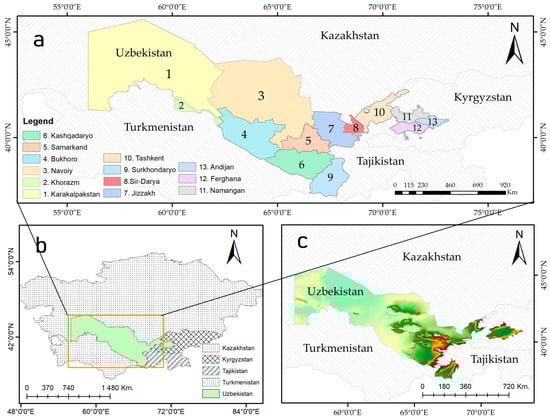
Figure 1.
The geographical location of the study area created using ArcMap software 10.8 (Environmental Systems Research Institute, Inc., California, United States of America): (a) map of the Uzbekistan highlighting each region of the country; (b) location of the study area in Central Asia; (c) digital elevation map (DEM) of the study area.
The total area of cotton in the country according to 2018 data is 10,830 km2 of land [41]. Cotton plantations are concentrated around Lake Aydar, which is located in central part of the country (near Bukhara), in Tashkent (North-East), along the Syr-Darya and Amu Darya (East) in the border region with Turkmenistan. The Fergana Valley is the most notable instance of large-scale irrigation systems in Central Asia. The main crop types in Uzbekistan are winter and summer cotton, wheat, corn, and rice. For instance, in 2017, more than 82.2% of planting fields were planted with cotton and wheat.
Sowing, seedling, squaring, flowering, boll development, and boll opening are the stages of cotton growth [42]. In this region, cotton is generally sown in late April and harvested in early September, after undergoing two main stages of vegetative and reproductive growth. Pictures of cotton at differing growth are shown in Figure 2, collected from the internet.
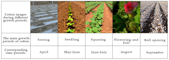
Figure 2.
Photographs of cotton at different growth stages.
2.2. Data and Processing
2.2.1. Remote Sensing Data
A time series of Sentinel-2 L2A satellite images from May to September 2018 was acquired from the Copernicus Data Space Ecosystem (https://dataspace.copernicus.eu/, accessed on 30 November 2023). Cloud percentage was confined to less than 10%. The image processing steps consisted of the following:
- Pan Sharpening to 10 m: This process improves the resolution of Sentinel-2’s 20 m and 60 m bands by merging them with the higher-resolution 10 m bands, resulting in clearer, more detailed images across all spectral bands.
- Projection to WGS-84: The satellite images are aligned with the WGS-84 geographic coordinate system, ensuring that the image data correspond accurately to real-world locations.
- Mosaic and Standard Map Divisions: Following the removal of overlaps and clouds, the images are stitched together into a single map (mosaic), then divided into standard segments for easier analysis.
Band information of Sentinel-2 L2A images is listed in Table 1.

Table 1.
Band information of Sentinel-2 L2A images.
2.2.2. Ground-Truth Data
We used a database of ‘ground-truth’ samples on crop types for Central Asia, where most of the data (97.7%) were collected in Uzbekistan [43]. The database consists of 8435 samples, where 40% or 3374 labels are cotton fields. A huge number of samples were collected between 2015 and 2018. Field surveys were conducted primarily in the Fergana Valley and reclamation area. Most were retrieved close to roadways, reflecting the inadequate accessibility within and between fields. During the field surveys, the following rules were observed to guarantee the representativeness of the samples:
- (1)
- The crop sample database composed of global positioning system (GPS) points collected initially, mainly near roads, highlighting poor field accessibility.
- (2)
- Single GPS point collected for each field, either at its accessible center or edges, and multiple points around obstructed field borders.
- (3)
- Image interpretation aided in drawing polygons around fields, utilizing high-resolution Google Earth satellite imagery.
- (4)
- Excluded non-vegetated areas, mixed-crop fields, and samples lacking valid Google Earth data due to observation limitations or cloud cover.
To ensure accuracy, all samples underwent additional verification by integrating time-series NDVI with phenological attributes. We used seasonal/annual spectral–temporal metrics and texture metrics to identify cotton lands. In order to obtain a newer dataset, we filtered the database and kept only samples for 2018. Therefore, the number of positive samples was reduced to 1077, and the sample distribution is depicted in Figure 3. This was carried out to avoid a large time gap between the sample collection year and our research time.
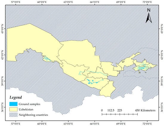
Figure 3.
Spatial distribution of ground samples in the study area. Only summer cotton samples for the year 2018 were chosen. The total number of ‘ground truth’ samples is 1077.
2.3. Methods
2.3.1. Automatic Sample Generation
We proposed a voting-based sample generation method for land delineation. In the event of lacking ground-truth data, automatically generated samples become essential, especially in large-scale extraction. Majority voting is an ML technique used to improve model accuracy and robustness by combining the predictions of multiple models in an ensemble, particularly for classification tasks. The final prediction is determined by the class that receives the most votes from the individual models. This approach helps in reducing overfitting, lowering variance, and ensuring more reliable predictions, especially in complex or noisy data scenarios.
The sample generation process, in general, encompasses a sequential progression comprising five distinct stages. The steps are described in Figure 4. Initially, Sentinel-2 images were acquired, followed by a targeted sampling of cotton based on the Uzbekistan crop database as a primary reference. Subsequently, a series of morphological analyses, including cloud dehaze and mosaic, were employed, then applied for the extraction of cropland edges using DexiNed architecture. Using a voting mechanism, the differentiation of cotton fields from other objects was executed. Finally, new samples were generated in accordance with these processes.
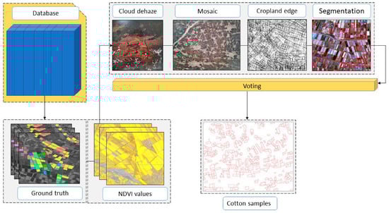
Figure 4.
The process of automatic generation of cotton samples using voting-based classification.
One of the main parts of sample generation is the detection of cropland edges. We used DexiNed [44] for this purpose since it is a specialized architecture designed for edge detection. DexiNed is engineered to enable training from beginning to end, without the necessity for initializing weights from pre-trained object detection models, as is common in most DL-based edge detectors. It comprises two distinct sub-networks: Dense Extreme Inception Network (Dexi) and the upsampling network (USNet). Dexi accepts an RGB image as input and processes it through various blocks. The feature maps generated from these blocks are then fed into USNet.
The satellite image was split into overlapping patches to reduce edge discrepancies, with central pixels in each patch given more weight using 2-D Gaussian interpolation. The final results were determined by a soft voting approach based on these weighted equations:
In Formula (1), the voting rule for each pixel involves , the weight of the prediction and the predicted probability for the class c. The weight varies with the pixel’s position relative to the center of the image. Formula (2) calculates based on the pixel coordinates. The total number of predictions depends on the pixel’s location in the original image.
Based on the described process, the segmented sections of each image patch were merged to create a complete, full-sized segmented image. This comprehensive image was then subjected to multiple processing stages to prepare it for subsequent application in obtaining samples:
- (1)
- The segmented results in the image are converted into vector format, maintaining the topology of the fields and their boundaries.
- (2)
- In this step, the boundaries delineated in the map are removed, leaving only the categories of agricultural fields and background.
The final vector data produced include numerous objects, depicted as polygons, that represent both agricultural fields and surrounding land parcels. Notably, areas adjacent to the field boundaries were intentionally omitted from these data.
2.3.2. An Adaptive Feature-Fusion Network
In this study, we used a novel adaptive feature-fusion network for crop classification using single-temporal Sentinel-2 Images [45]. The selective path module was developed to address complex scenarios. It incorporates an adaptive approach, whereby features extracted from multiple patch sizes are combined, allowing for the integration of contextual information at varying scales. Spectral information of the central pixel of the patches was extracted using TabNet [46]. The adaptive feature-fusion network uses multitask learning to supervise the extraction phase to improve the weight of the spectrum features and alleviate the negative impact of insufficient samples.
In order to achieve more accurate results, we added an attention model to the fusion network. This helps to improve long-range dependencies, reduce information loss, provide adaptability, and offer interpretability. This modification aligns with our goal of optimizing the network’s performance and boosting its capabilities since our task requires nuanced understanding and selective attention to specific features.
The SPTNet architecture of the network introduces a selective patch module (SPM) for acquiring adaptive multi-size patch features, alongside a TabNet branch that handles spectral data of center points and multiple loss functions. This approach enhances spatial information while minimizing noise through patch fusion. The architecture incorporates multitask learning to emphasize spectral details through added loss. This refines crop plot boundaries and mitigates mixed pixel interference, improving overall model performance. The SPTNet framework combines these elements to effectively enhance image analysis for crop identification.
Figure 5 shows the workflow of crop classification based on an adaptive feature fusion network. This classification framework consists of three steps:
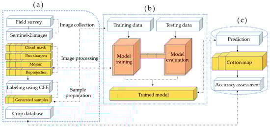
Figure 5.
Framework for mapping cotton fields. Whole process consists of three main steps: (a) data collection and preparation; (b) training and testing the data; (c) mapping and accuracy assessment.
- Data collection and sampling.
- Training and evaluation of the model.
- Prediction, cotton field mapping, and accuracy assessment.
2.3.3. Selective Patch Module
Due to the varying sizes of crop plots across different scenarios, the utilization of oversized patches introduces a surplus of pixels that differ from the central pixel’s category, possibly leading to the misclassification of certain pixels as noise. Conversely, opting for patches that are excessively small results in an insufficient spatial information pool, thereby compromising classification precision. The module addresses a scale-dependence issue analogous to the receptive field dilemma in semantic segmentation. Whereas receptive field manipulation is employed there, this method involves adaptive patch size selection to extract multi-scale features commensurate with the target. SK-Conv [47] stands as a solution by autonomously determining the convolutional receptive field. Various studies have employed SK-Conv, which computes the weight of feature maps generated by convolution kernels of diverse dimensions, merging the maps based on these weights to achieve an adaptable selection of the convolutional kernel receptive field.
Just like the SK-Conv technique, this method devises a Spatial Pyramid Module (SPM) to dynamically amalgamate features from distinct patch sizes. The framework is shown in Figure 6. This innovation serves to address scalability challenges while garnering more precise spatial insights. The SPM comprises three key stages: split, fusion, and selection. This tripartite arrangement optimizes the generation of diverse patch sizes, as well as the aggregation of patch details to derive a comprehensive representation of selection weight. Consequently, feature maps of various patch sizes are obtained according to this weight.
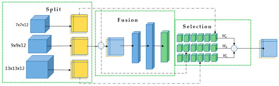
Figure 6.
The framework of the selective patch module.
The split phase initiates the process by segmenting input patches into , and based on prescribed dimensions. In our study on crop classification in Uzbekistan, we employed patch sizes of 7 × 7, 9 × 9, and 13 × 13 pixels, aligning with the regional land scale. The ensuing fusion stage involves two convolutions on the patches to generate equivalent-sized feature maps , and . Subsequently, the fusion stage combines information from different branches, yielding U = . To infuse global context and establish channel statistics for , global average pooling is applied. Employing the full connection layer reduces the dimension of channel statistics and yields the ultimate channel weight , as expressed by Formula (3):
Concluding this process, the selection phase involves the creation of three weight matrices: , and . These matrices are derived from the final channel weight z, ensuring coherence through the application of the softmax function. The module enforces a constraint, and the sum of corresponding elements across weight matrices is normalized to one. Subsequently, these weight matrices are employed to assign weights to the feature maps , and . The result is an adaptively chosen spatial feature, denoted as V, which is obtained by summing the weighted feature maps. This entire sequence of operations is encapsulated by Formulas (4) and (5):
2.3.4. Loss Function
Choosing the right loss function is critical for guiding the optimization process and converging to an accurate model. The loss function used to optimize the neural network has two components. In this study, we utilized cross-entropy loss as it is commonly applied for multi-class classification tasks. Cross-entropy loss measures the difference between the predicted class probabilities and the true labels. It is widely used because its value depends only on the probability of the correct class, making it convenient to calculate and optimize. The cross-entropy loss sums the negative log probabilities of the true target classes based on Formula (6):
In Formula (6), “” represents the true label value, “” signifies the classification probability, and “N” corresponds to the number of classes. The overall loss function of the network comprises two branch loss functions, and this depicted as:
In the context of Formula (7), where the total loss is a combination of two cross-entropy (CE) loss functions ( and ), the use of and as coefficients serves to balance the contribution of each loss function to the total loss. This approach allows for fine-tuning the model’s learning process.
Utilizing two separate loss functions can address different aspects of the learning task or handle distinct types of data within the model. The values for and , which sum up to 1, determine the relative importance of each loss function. Adjusting these values can help in emphasizing one aspect of learning over another, depending on the specific requirements of the classification task. For example, if is more critical for model performance, would be set higher than .
2.3.5. Random Forest Classifier
For method comparison, we chose RF [48] algorithm. It has demonstrated considerable effectiveness across numerous RS applications, such as land cover change detection, crop mapping, and estimation of soil constituents [49,50]. It has been proved to be one of the most efficient ML techniques for classification tasks [51,52,53]. Its algorithms work by aggregating the predictions from multiple decision tree models to generate an overall output [54]. As shown in Figure 7, unlike decision tree algorithms that construct a single tree for making predictions, RF creates numerous decision trees during training and then averages their probabilistic predictions to make a final classification or regression prediction.
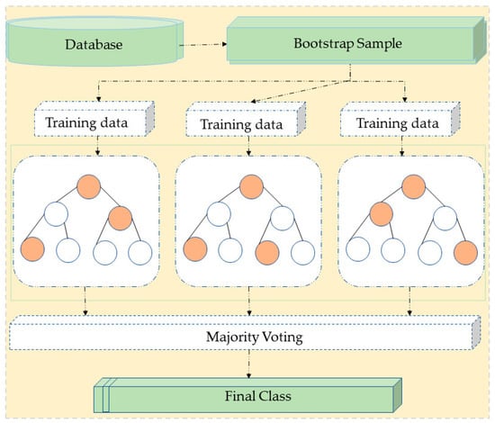
Figure 7.
Principle of the Random Forest (RF) classifier.
As this research aims to assess specific phenology-related measurements that could assist in identifying cotton through surface reflectance data, only two categories of land cover were created: cotton and non-cotton. The non-cotton class combined multiple land cover types, like bare soil, water, other crops, pastures, and native vegetation. In the conducted study, various RF models were established with varying numbers of decision trees. The assessment criteria employed to explore the ideal number of decision trees encompassed both the OA and the KC. Through an analysis of model accuracies, a count of 23 decision trees was chosen as optimal.
Furthermore, the number of features utilized for each split was determined to be the square root of the total input features. In the conducted experiments, the data fed into both the RF and SPTNet consisted of a vector with a size of 1 × 12, representing the values of 12 different spectral bands for an individual pixel. In the experiment, all deep learning methods used a 7 × 7 × 12 vector for input. This represents a patch with the central pixel having a size of 7, capturing a comprehensive array of spectral data across 12 different bands for each pixel within the 7 × 7 area. The other parameters used in the model were set to their default values without modification.
The RF was implemented using the Scikit-learn open-source Python library. Scikit-learn provides a diverse set of machine learning modules and capabilities [55]. Using Scikit-learn makes it easy and efficient to implement ML workflows, including data loading, dividing data into training and validation sets, preprocessing, and applying learning algorithms.
2.4. Analysis and Sampling
2.4.1. Feature Preparation
The Google Earth Engine (GEE) offers a comprehensive cloud-based platform for effortless access and efficient processing of vast quantities of openly accessible satellite imagery [56]. This includes imagery procured by the Sentinel-2 satellite, presenting a powerful tool for researchers and analysts in the fields of Earth observation and geospatial analysis. The GEE includes some of the most advanced classification algorithms for pixel-based classification that can be implemented in agricultural mapping applications [57]. For instance, we used GEE to calculate NDVI and VH spectra in classified regions. The results are presented in Figure 8 and Figure 9.
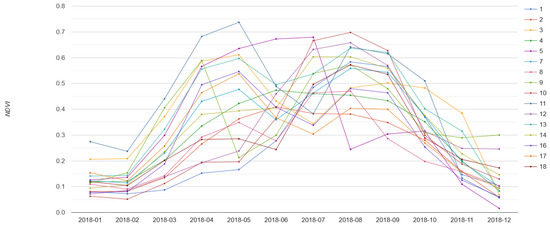
Figure 8.
Sentinel-2 normalized difference vegetation index (NDVI) spectra of cotton in Uzbekistan for each month of 2018 obtained with google earth engine (GEE).
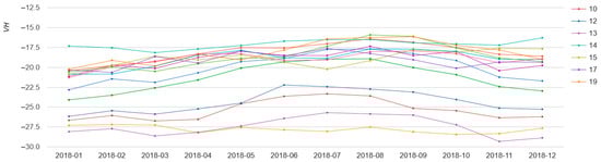
Figure 9.
Temporal Synthetic Aperture Radar (SAR) backscatter profile (VH polarization) of sample cotton fields in Uzbekistan for each month of 2018 obtained with GEE.
2.4.2. Sampling Process
In addition to ‘ground truth’ data, we added another 200 cotton and 400 non-cotton samples using GEE (Figure 10). Satellite imagery was collected throughout the full crop growing season in order to obtain the spectral reflectance measurements across different bands for each pixel. Using this time series of multi-spectral images, the Normalized Difference Vegetation Index (NDVI) was derived per pixel by calculating the normalized ratio between the near-infrared and red spectral bands [58] (Formula (8)):
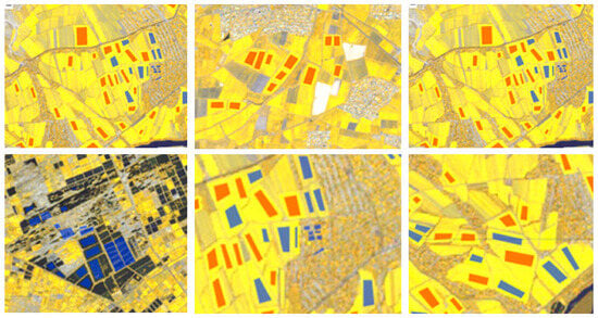
Figure 10.
Sampling process in GEE. Band-8, band-6, and band-4 of Sentinel-2 images are composited to increase the variability of the cotton crop from other features. Red polygons represent positive samples (cotton), blue polygons—negative (non-cotton). Negative samples include other crops, forests, roads etc.
2.5. Accuracy Assessment
In order to evaluate the accuracy of classification, a high-quality verification database at an appropriate spatial and temporal scale should be obtained. Thus, such verification databases are a critical element of the mapping process [59]. In our research, the main source of accuracy assessment was a dataset of crop types in Central Asia [43]. Among 8435 samples of different crops, 4025 were cotton. We utilized Sentinel-2 imagery and GEE to identify and sample non-cotton fields. Using these tools, we drew rectangles over the areas of interest in the satellite imagery to sample fields that did not contain cotton. This sampling included a variety of other crops and also encompassed different ground objects such as roads and buildings. This comprehensive approach allowed us to accurately categorize and analyze various land uses and cover types beyond just agricultural fields. We then added automatically generated samples to the database.
A confusion matrix was used to analyze the classification results. It is a common format for assessing crop classification accuracy. The first metric we used was producer accuracy (PA), which is a performance metric that evaluates a model’s ability to correctly classify positive instances out of all instances predicted as positive. The second evaluation metric was user accuracy (UA), which is the proportion of pixels correctly classified into the class compared to the total count of pixels classified to that class. The OA signifies the ratio of pixels that have been accurately classified to the total number of pixels. Lastly, the kappa coefficient (KC) serves as an indicator of consistency and can also be employed to assess the impact of classification. We also used F1 score for evaluation purposes. To better measure categorization accuracy, the F1 score, which considers the accuracy and recall rate, is a regularly used evaluation index.
Formulas are shown below:
In Formulas (9)–(11) above, true positive (TP) refers to correctly identified pixels that were indeed positive cases. False positives (FP) correspond to positive pixels that were inaccurately categorized. A false negative (FN) represents a negative pixel that has been mistakenly classified.
2.6. Training Details
We implemented all the deep neural networks in this study using the Pytorch DL library. The training and validation data samples were used to train the models on an NVIDIA GeForce RTX 3090 GPU with 24 GB memory. During model training, the batch size was 256, optimization was via the Adam [60] algorithm, the initial learning rate was 0.001, and cosine annealing [61] was used to gradually reduce the learning rate. For the hyperparameter setting of the loss function, we set the values of λ1 to 0.7 and λ2 to 0.3.
3. Results
3.1. Automatically Generated Samples
An example of the obtained results of agricultural parcel land of Uzbekistan is shown in Figure 11. The red regions shown in the figure indicate parcels, illustrating the potential for automatically creating training samples using existing multisource RS products. Utilizing the proposed collection strategy significantly enhanced the representativeness of training samples. The DexiNed edge detection method was effectively employed to delineate crop boundaries in Uzbekistan, providing a clear demarcation of agricultural fields. The model demonstrated high performance in identifying field boundaries.
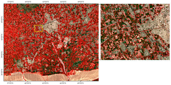
Figure 11.
Agricultural parcel land map produced by DexiNed model.
Next, we used a voting mechanism to distinguish cotton from other objects on the ground. The results of the obtained vector samples are shown in Figure 12. In every classified map, the central pixel’s label undergoes refinement based on the majority voting rule applied within a flexible region, a process known as adaptive majority voting. This refinement is carried out methodically for each pixel across the initial classified maps.
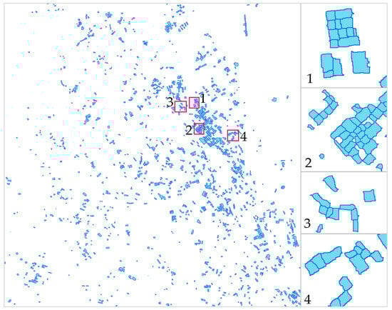
Figure 12.
Results of obtained cotton samples using proposed voting-based classification. Each rectangle in the image highlights the obtained cotton samples.
3.2. Spatial Distribution of Cotton Fields
The results of mapping cotton fields in the study area are depicted in Figure 13. This includes the classification maps generated from the Sentinel-2 images for 2018. The model was trained by automatically generated samples and evaluated using ground-truth data. Our results show that the total area of cotton fields in Uzbekistan is 1148 thousand hectares. Cotton fields are distributed across all provinces and regions, and the smallest cotton planting areas are Kashqadaryo, Surkhandaryo, Bukhoro, and Sir-Darya. The cotton field planting areas in the counties Tashkent, Khorazm, and Bukhoro were the largest ones (Figure 14).
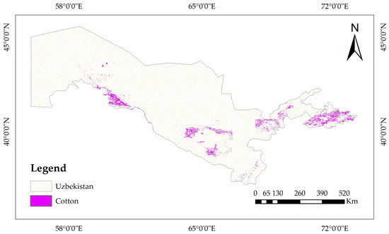
Figure 13.
Spatial distribution of cotton in Uzbekistan for year 2018 obtained with automatically generated samples, using adaptive feature fusion network and Sentinel-2 imagery.
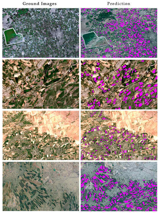
Figure 14.
Examples of predicted cotton fields in Uzbekistan for 2018.
3.3. Classification Accuracy Assessment
In the creation of the cotton distribution map for Uzbekistan in 2018 using SPTNet, validation of the mapping outcomes was critically important. To achieve this, this study used statistical data obtained from the State Statistics Committee of Uzbekistan (https://stat.uz/, accessed on 30 November 2023), which presumably provided official data on cotton production, including the area of cultivation and yield for 2018. These statistics were instrumental in the validation process, where cross-validation techniques were employed. This process involved comparing the SPTNet mapping results with the official data to assess accuracy, ensuring that the cotton distribution map reliably reflected the actual cotton production scenario in Uzbekistan.
The accuracy assessed using cross-validation is presented in Figure 15.
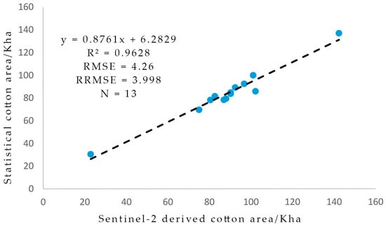
Figure 15.
Illustration of the contrast between the cotton cultivation area determined from Sentinel-2 imagery and the statistical data on a sub-national level in Uzbekistan for the year 2018.
Precision–recall (PR) curves are presented in Figure 16, where the area under the curve (AUC) equals 0.91. PR curves allow us to visualize the tradeoff between precision and recall that results from choosing different probability thresholds, gaining insight into model performance that single metrics like accuracy cannot provide.
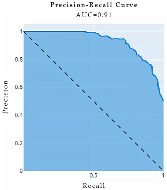
Figure 16.
A Precision–recall (PR) curve with area under the curve (AUC) = 0.91. By examining the shape and slope of the curve, we can assess how well a model separates classes and calibrates its predictions.
To make a comparison with the statistical data regarding the cotton area, the count of cotton pixels identified from the mapping results was computed for each state and subsequently multiplied by the size of the Sentinel-2 pixel, as described in Figure 17. The cotton areas in 2018, derived from Sentinel-2 data using the proposed method, were 1148 thousand hectares. A minor overestimation was observed when comparing these results with the statistical cotton areas, with a relative error of 5.60%.
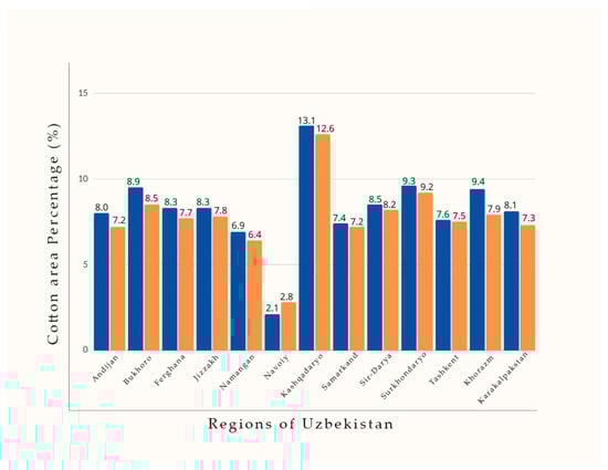
Figure 17.
The percentage of cotton area within each state concerning the overall cotton area in Uzbekistan during the year 2018. Blue color represents our results, orange color is official statistics.
Most regions experienced a slight overestimation in cotton areas, with Khorazm state showing notable overestimations. Conversely, Navoiy state had an underestimation in cotton areas. The classification results at different phases of cotton vegetation are shown in Figure 18.
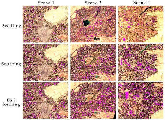
Figure 18.
Results of cotton classification at seedling, squaring and ball forming stages.
As a result, we received a 10 m distribution map for cotton fields in Uzbekistan based on an adaptive feature fusion network for crop classification using Sentinel-2. Validation samples were used to perform accuracy evaluations on the resulting cotton field map, revealing that the extracted map from this study exhibited a notably high level of accuracy. The highest results were achieved in August. The obtained results exceeded the accuracy of existing cotton maps of Uzbekistan. The confusion matrix results are shown in Table 2.
Table 2.
Confusion matrix of the cotton map in August for Uzbekistan.
An OA of 0.947, producer accuracy of 0.854, UA of 0.838, KC of 0.795, and F1 score of 0.953 were achieved. The obtained results are consistent with statistical data for cotton fields in Uzbekistan in 2018. The estimated total cropland area reached 11 840 km2 for 650 km2, higher than the statistical cropland area.
3.4. Optimal Classification Phase
One of the main objectives of this study was to identify the most suitable phases for cotton field mapping. This could potentially streamline the process of crop classification by narrowing down the focus to specific phenological phases of the cotton in the study area [62]. The cotton fields were extracted based on single-phase data from May to September. As mentioned above, our results demonstrated that in the event of single-phase data extraction, mapping cotton land based on the data in the boll-forming phase was highly accurate. In the period of boll forming, the characteristics of cotton differed significantly from those of other crops. Therefore, the accuracy of the cotton map in August was the highest, with an OA of 0.947 and KC of 0.795, respectively (Table 3). On the other hand, the precision of the cotton field map derived from seedling phase data was the lowest, registering an OA of 0.865 and a KC of 0.526. Cotton shares similarities with the attributes of other crops in the corresponding growth period, such as corn.
Table 3.
Accuracy of the cotton field extraction for SPTNet during phases of cotton vegetation.
The results for RS show that in the case of single-phase extraction, SPTNet is notably better than RS. On the other hand, the outcomes of the data extraction approach with RF for cotton fields revealed that merging the images captured in June and August led to improved accuracy, resulting in an OA of 0.929 and a KC of 0.789. During both of these months, the cotton was in distinct stages: the late seedling stage in one case and the early boll-opening stage in the other. This disparity in growth stages resulted in notable dissimilarities in the RS attributes of cotton fields, as compared to other crops.
As a result, the incorporation of multi-phase data from June and August facilitated the classification technique in mitigating redundancy in features during the cotton field extraction procedure, subsequently lightening the workload related to image processing. This optimization significantly bolstered the efficiency of the cotton field extraction process. Consequently, this approach enabled the precise delineation of cotton fields with heightened accuracy during the boll-opening period in August. Cotton harvesting in Uzbekistan usually takes place at the end of September and early October; therefore, the mapping work can be established about 35 to 40 days before harvest. This would offer punctual and precise judgments that aid in effectively distributing labor resources for the cotton harvesting process across different spatial areas (Table 4).
Table 4.
Accuracy of the cotton field extraction for RF during single and multi-temporal data extraction.
Using RF with the multi-temporal data extraction showed that combining data in June and August, June and July, and July and August could achieve better accuracy compared to RF single-phase extraction. The OAs for these three months were 0.924, 0.929, and 0.927, respectively, with the combination of June and August achieving the highest accuracy among them.
3.5. Comparison of SPTNet and RF Results
In Figure 19, we performed analyses to compare the crop maps of Uzbekistan generated using SPTNet against those produced by RF. It relies solely on spectral data of individual pixels, without considering spatial or temporal context. In our experiments, the input was a 1 × 12 vector of pixel reflectance values across 12 spectral bands. We used the combined CNN-RF method, which initially extracts features via a CNN before employing RF for classification. This approach harnesses the strengths of both techniques to enhance the model’s generalization capability, thereby capitalizing on the benefits offered by each method.
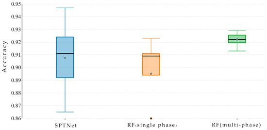
Figure 19.
Accuracy comparison of the SPTNet with RF. Boxplots represent the median (horizontal line), mean (◦), as well as the lower and upper quartiles (extremities of each box) of the data.
The results showed that SPTNet reaches higher accuracy compared to RF in cotton classification at a large scale. The highest OA for RF was 0.929, obtained in June and August, while for SPTNet, it reached 0.947, obtained in August.
4. Discussion
4.1. Advantages and Limitations
Mapping crops with high resolution over extensive agricultural areas presents a significant difficulty in the field of RS. In this research, we used an adaptive feature-fusion network that is reliable for extracting crops on a large scale. The network achieves a high classification accuracy using solely single-temporal Sentinel-2 images. Compared to other well-known methods, our network does not require a huge number of samples.
It is worth mentioning that the SPTNet has the capability to dynamically adjust and combine spatial information based on the plot size in a real-world scenario. This adaptability ensures that the system is able to effectively capture and extract small and intricate features, even in varying conditions. The ability to adapt and extract small features in near-real-time scenarios provides timely decision support to farmers, enabling them to respond quickly to changing conditions and optimize their crop management strategies. It is worth mentioning that the processing speeds were fast considering the massive dataset, extensive timeframe, and broad region studied. It took a mere 26 h to analyze the entire country using a readily available computer.
Even though the cotton map created for Uzbekistan at a 10 m resolution exhibited a notable level of accuracy, it is important to acknowledge the presence of certain limitations and uncertainties [63]. One of the main limitations pertains to the accessibility of images of critical phenological stages. One potential way to improve future research would be to integrate Sentinel-2 data with additional RS sources, like MODIS, RapidEye, and Landsat, to acquire more complete and complementary observations. Fusing multi-platform satellite imagery could help mitigate the constraints posed by limited revisit frequency and cloud contamination in Sentinel-2 data alone. The combined strengths of diverse sensors like the high resolution of Landsat and the large coverage of Sentinel-2 may enable more robust analyses.
Thirdly, this study focused only on the adaptive feature-fusion network and RF classifier while excluding other ML and DL algorithms like XGBoost, SVM, etc. Since no single model works best for all cases, future efforts could enhance accuracy by using a multi-classifier system that combines diverse models.
4.2. Future Perspectives
This study utilized Sentinel-2 imagery for its high spectral resolution to automatically generate cotton samples and perform cotton field classification. Additionally, high-resolution satellite data were leveraged for their detailed spatial resolution to plot field boundaries. The high spectral resolution enables identifying crops, while the spatial resolution supports extracting field edges precisely [64]. Combining these complementary strengths of the multi-resolution data will potentially improve the overall performance of crop-type classification within accurately mapped agricultural plot boundaries. The integration of detailed plot-level delineation and crop-type classification is an area worth exploring further.
4.3. Future Research
Future research may involve integrating Synthetic Aperture Radar (SAR) data into the crop classification process of the network. SAR satellites possess the capability to capture images, regardless of weather conditions, compensating for the absence of optical data. Additionally, SAR data’s sensitivity to crop canopy structure and water content holds the potential to enhance the distinctive features utilized in crop classification, thereby contributing to an elevated level of classification accuracy [65,66].
This approach allows for mapping not just cotton but various other crops as well. At the same time, there is a diversification of agricultural produce in Uzbekistan, evidenced by the transformation of cotton fields into areas cultivating different types of crops. Wheat, soybean, and corn are a few of them. The proposed method has proven to be effective for crop classification at a large scale.
5. Conclusions
The automated generation of cotton samples proves to be an indispensable asset in expediting and refining the training process of machine and DL models for RS applications. Training the model using automatically generated samples proved to have satisfactory accuracy. Additionally, acquiring information about the planting area and spatial distribution of cotton fields holds vital importance for ensuring timely and precise agricultural management practices in Uzbekistan. Therefore, this research assessed the potential of Sentinel-2 imagery and DL techniques for large-scale cotton field classification. We used an adaptive feature-fusion network to assess the ability of the Sentinel-2 satellite to detect cotton fields at the country level. Employing the suggested framework, we created a cotton field map for Uzbekistan in 2018, with a spatial resolution of 10 m. The experiment achieved an OA of 0.947, indicating that the results are in alignment with the statistical data for cotton fields in Uzbekistan for 2018. When comparing the obtained results with the official statistical cotton areas, a minor overestimation was observed. This discrepancy amounted to a relative error of 5.60% or 650 km2. Based on the results and analyses, we reached the following results and conclusions:
- (1)
- The results show that voting-based classification is a reliable choice for sample generation.
- (2)
- The classification models were predominantly influenced by phenological features based on dates.
- (3)
- In the case of single-phase mapping with SPTNet, August was the most suitable month for mapping cotton in Uzbekistan. The combination of June and August achieved the highest accuracy in the case of multi-temporal data extraction using RF.
- (4)
- We obtained a 10 m Sentinel-2 cotton map of Uzbekistan for 2018 using an adaptive feature-fusion network.
Two methods were used to evaluate the results. Firstly, the ground-truth database for different crops obtained in 2018 was used for reference data. Secondly, we compared the obtained results with the official statistics of the country for 2018. The accuracy assessment showed that the classification of cotton fields using the proposed method had high OA. Our classification results highlight the boll-opening stage as a significant phenological stage for cotton identification.
Although the current study focused on detecting cotton fields in Uzbekistan, its applicability could extend to other geographic regions and other crop types. It is important to note, however, that the approach relies on “ground truth” data, which may limit its usability in areas where such data are scarce.
Author Contributions
Conceptualization, Y.G. and Z.C.; methodology, X.T. and Y.B.; validation, J.J. and X.T.; formal analysis, Y.G.; resources, Z.C. and S.W.; data curation, Y.B. and Y.L.; writing—original draft preparation, Y.B. and J.J.; writing—review and editing, J.J.; visualization, J.J.; supervision, J.J.; project administration, Z.C.; funding acquisition, Z.C. All authors have read and agreed to the published version of the manuscript.
Funding
This study was supported by the National Key Research and Development Program of China (No. 2021YFB3901300).
Data Availability Statement
Data are contained within the article.
Acknowledgments
The authors are grateful to the editors and anonymous reviewers for their informative suggestions.
Conflicts of Interest
The authors declare no conflicts of interest.
Abbreviations
The following abbreviations are used in this manuscript:
| RS | remote sensing |
| ML | machine learning |
| DL | deep learning |
| CE | cross entropy |
| OA | overall accuracy |
| GEE | google earth engine |
| CNN | convolutional neural network |
| FN | false negative |
| FP | false positive |
| KC | kappa coefficient |
| NDVI | normalized difference vegetation index |
| PA | producer accuracy |
| SPM | selective patch module |
| TP | true positive |
| UA | user accuracy |
| PR | precision recall |
| AUC | area under the curve |
References
- Djanibekov, N.; Rudenko, I.; Lamers, J.; Bobojonov, I. Pros and Cons of Cotton Production in Uzbekistan. In Food Policy for Developing Countries: Food Production and Supply Policies, Case Study No. 7–9; CUL Initiatives in Publishing (CIP): Ithaca, NY, USA, 2010; p. 13. [Google Scholar]
- Morawska, E. Cotton Industry in Uzbekistan: The Soviet Heritage and the Challenge for Development of the Country; Academia.edu. 2017. Available online: https://www.academia.edu/78867844/Cotton_industry_in_Uzbekistan_the_Soviet_heritage_and_the_challenge_for_development_of_the_country (accessed on 17 November 2023).
- Alves, A.N.; Souza, W.S.R.; Borges, D.L. Cotton Pests Classification in Field-Based Images Using Deep Residual Networks. Comput. Electron. Agric. 2020, 174, 105488. [Google Scholar] [CrossRef]
- Razzaq, A.; Zafar, M.M.; Ali, A.; Hafeez, A.; Batool, W.; Shi, Y.; Gong, W.; Yuan, Y. Cotton Germplasm Improvement and Progress in Pakistan. J. Cotton Res. 2021, 4, 1. [Google Scholar] [CrossRef]
- Ho, T.T.K.; Tra, V.T.; Le, T.H.; Nguyen, N.-K.-Q.; Tran, C.-S.; Nguyen, P.-T.; Vo, T.-D.-H.; Thai, V.-N.; Bui, X.-T. Compost to Improve Sustainable Soil Cultivation and Crop Productivity. Case Stud. Chem. Environ. Eng. 2022, 6, 100211. [Google Scholar] [CrossRef]
- Liu, Z.; Yang, P.; Tang, H.; Wu, W.; Zhang, L.; Yu, Q.; Li, Z. Shifts in the Extent and Location of Rice Cropping Areas Match the Climate Change Pattern in China during 1980–2010. Reg. Environ. Chang. 2015, 15, 919–929. [Google Scholar] [CrossRef]
- Zhong, L.; Hu, L.; Yu, L.; Gong, P.; Biging, G.S. Automated Mapping of Soybean and Corn Using Phenology. ISPRS J. Photogramm. Remote Sens. 2016, 119, 151–164. [Google Scholar] [CrossRef]
- Al-Shammari, D.; Fuentes, I.; Whelan, B.M.; Filippi, P.; Bishop, T.F.A. Mapping of Cotton Fields Within-Season Using Phenology-Based Metrics Derived from a Time Series of Landsat Imagery. Remote Sens. 2020, 12, 3038. [Google Scholar] [CrossRef]
- Bendini, H.; Sanches, I.D.; Körting, T.S.; Fonseca, L.M.G.; Luiz, A.J.B.; Formaggio, A.R. Using landsat 8 image time series for crop mapping in a region of cerrado, Brazil. Int. Arch. Photogramm. Remote Sens. Spat. Inf. Sci. 2016, XLI-B8, 845–850. [Google Scholar] [CrossRef][Green Version]
- Schmidt, M.; Pringle, M.; Devadas, R.; Denham, R.; Tindall, D. A Framework for Large-Area Mapping of Past and Present Cropping Activity Using Seasonal Landsat Images and Time Series Metrics. Remote Sens. 2016, 8, 312. [Google Scholar] [CrossRef]
- do Nascimento Bendini, H.; Garcia Fonseca, L.M.; Schwieder, M.; Sehn Körting, T.; Rufin, P.; Del Arco Sanches, I.; Leitão, P.J.; Hostert, P. Detailed Agricultural Land Classification in the Brazilian Cerrado Based on Phenological Information from Dense Satellite Image Time Series. Int. J. Appl. Earth Obs. Geoinf. 2019, 82, 101872. [Google Scholar] [CrossRef]
- Pan, Z.; Huang, J.; Zhou, Q.; Wang, L.; Cheng, Y.; Zhang, H.; Blackburn, G.A.; Yan, J.; Liu, J. Mapping Crop Phenology Using NDVI Time-Series Derived from HJ-1 A/B Data. Int. J. Appl. Earth Obs. Geoinf. 2015, 34, 188–197. [Google Scholar] [CrossRef]
- Carletto, C.; Gourlay, S.; Winters, P. From Guesstimates to GPStimates: Land Area Measurement and Implications for Agricultural Analysis. J. Afr. Econ. 2015, 24, 593–628. [Google Scholar] [CrossRef]
- Zhang, J.; Feng, L.; Yao, F. Improved Maize Cultivated Area Estimation over a Large Scale Combining MODIS–EVI Time Series Data and Crop Phenological Information. ISPRS J. Photogramm. Remote Sens. 2014, 94, 102–113. [Google Scholar] [CrossRef]
- Khanal, S.; Kc, K.; Fulton, J.P.; Shearer, S.; Ozkan, E. Remote Sensing in Agriculture—Accomplishments, Limitations, and Opportunities. Remote Sens. 2020, 12, 3783. [Google Scholar] [CrossRef]
- Pradhan, S. Crop Area Estimation Using GIS, Remote Sensing and Area Frame Sampling. Int. J. Appl. Earth Obs. Geoinf. 2001, 3, 86–92. [Google Scholar] [CrossRef]
- Weiss, M.; Jacob, F.; Duveiller, G. Remote Sensing for Agricultural Applications: A Meta-Review. Remote Sens. Environ. 2020, 236, 111402. [Google Scholar] [CrossRef]
- Hu, Q.; Sulla-Menashe, D.; Xu, B.; Yin, H.; Tang, H.; Yang, P.; Wu, W. A Phenology-Based Spectral and Temporal Feature Selection Method for Crop Mapping from Satellite Time Series. Int. J. Appl. Earth Obs. Geoinf. 2019, 80, 218–229. [Google Scholar] [CrossRef]
- Toth, C.; Jóźków, G. Remote Sensing Platforms and Sensors: A Survey. ISPRS J. Photogramm. Remote Sens. 2016, 115, 22–36. [Google Scholar] [CrossRef]
- Justice, C.O.; Townshend, J.R.G.; Vermote, E.F.; Masuoka, E.; Wolfe, R.E.; Saleous, N.; Roy, D.P.; Morisette, J.T. An Overview of MODIS Land Data Processing and Product Status. Remote Sens. Environ. 2002, 83, 3–15. [Google Scholar] [CrossRef]
- Loveland, T.R.; Dwyer, J.L. Landsat: Building a Strong Future. Remote Sens. Environ. 2012, 122, 22–29. [Google Scholar] [CrossRef]
- Song, X.-P.; Huang, W.; Hansen, M.C.; Potapov, P. An Evaluation of Landsat, Sentinel-2, Sentinel-1 and MODIS Data for Crop Type Mapping. Sci. Remote Sens. 2021, 3, 100018. [Google Scholar] [CrossRef]
- Phiri, D.; Simwanda, M.; Salekin, S.; Nyirenda, V.R.; Murayama, Y.; Ranagalage, M. Sentinel-2 Data for Land Cover/Use Mapping: A Review. Remote Sens. 2020, 12, 2291. [Google Scholar] [CrossRef]
- Segarra, J.; Buchaillot, M.L.; Araus, J.L.; Kefauver, S.C. Remote Sensing for Precision Agriculture: Sentinel-2 Improved Features and Applications. Agronomy 2020, 10, 641. [Google Scholar] [CrossRef]
- Vuolo, F.; Neuwirth, M.; Immitzer, M.; Atzberger, C.; Ng, W.-T. How Much Does Multi-Temporal Sentinel-2 Data Improve Crop Type Classification? Int. J. Appl. Earth Obs. Geoinf. 2018, 72, 122–130. [Google Scholar] [CrossRef]
- Yang, H.; Pan, B.; Li, N.; Wang, W.; Zhang, J.; Zhang, X. A Systematic Method for Spatio-Temporal Phenology Estimation of Paddy Rice Using Time Series Sentinel-1 Images. Remote Sens. Environ. 2021, 259, 112394. [Google Scholar] [CrossRef]
- Hu, T.; Hu, Y.; Dong, J.; Qiu, S.; Peng, J. Integrating Sentinel-1/2 Data and Machine Learning to Map Cotton Fields in Northern Xinjiang, China. Remote Sens. 2021, 13, 4819. [Google Scholar] [CrossRef]
- Chen, Y.; Lu, D.; Moran, E.; Batistella, M.; Dutra, L.V.; Sanches, I.D.; da Silva, R.F.B.; Huang, J.; Luiz, A.J.B.; de Oliveira, M.A.F. Mapping Croplands, Cropping Patterns, and Crop Types Using MODIS Time-Series Data. Int. J. Appl. Earth Obs. Geoinf. 2018, 69, 133–147. [Google Scholar] [CrossRef]
- Goldberg, K.; Herrmann, I.; Hochberg, U.; Rozenstein, O. Generating Up-to-Date Crop Maps Optimized for Sentinel-2 Imagery in Israel. Remote Sens. 2021, 13, 3488. [Google Scholar] [CrossRef]
- Lambert, M.-J.; Traoré, P.C.S.; Blaes, X.; Baret, P.; Defourny, P. Estimating Smallholder Crops Production at Village Level from Sentinel-2 Time Series in Mali’s Cotton Belt. Remote Sens. Environ. 2018, 216, 647–657. [Google Scholar] [CrossRef]
- Grabska, E.; Hostert, P.; Pflugmacher, D.; Ostapowicz, K. Forest Stand Species Mapping Using the Sentinel-2 Time Series. Remote Sens. 2019, 11, 1197. [Google Scholar] [CrossRef]
- Traganos, D.; Reinartz, P. Mapping Mediterranean Seagrasses with Sentinel-2 Imagery. Mar. Pollut. Bull. 2018, 134, 197–209. [Google Scholar] [CrossRef]
- Maggiori, E.; Tarabalka, Y.; Charpiat, G.; Alliez, P. Convolutional Neural Networks for Large-Scale Remote-Sensing Image Classification. IEEE Trans. Geosci. Remote Sens. 2017, 55, 645–657. [Google Scholar] [CrossRef]
- Heung, B.; Ho, H.C.; Zhang, J.; Knudby, A.; Bulmer, C.E.; Schmidt, M.G. An Overview and Comparison of Machine-Learning Techniques for Classification Purposes in Digital Soil Mapping. Geoderma 2016, 265, 62–77. [Google Scholar] [CrossRef]
- Chen, Y.; Lin, Z.; Zhao, X.; Wang, G.; Gu, Y. Deep Learning-Based Classification of Hyperspectral Data. IEEE J. Sel. Top. Appl. Earth Obs. Remote Sens. 2014, 7, 2094–2107. [Google Scholar] [CrossRef]
- Song, X.; Yang, C.; Wu, M.; Zhao, C.; Yang, G.; Hoffmann, W.C.; Huang, W. Evaluation of Sentinel-2A Satellite Imagery for Mapping Cotton Root Rot. Remote Sens. 2017, 9, 906. [Google Scholar] [CrossRef]
- Feng, A.; Zhou, J.; Vories, E.; Sudduth, K.A. Evaluation of Cotton Emergence Using UAV-Based Imagery and Deep Learning. Comput. Electron. Agric. 2020, 177, 105711. [Google Scholar] [CrossRef]
- Khan, R.U.; Zhang, X.; Kumar, R.; Aboagye, E.O. Evaluating the Performance of ResNet Model Based on Image Recognition. In Proceedings of the 2018 International Conference on Computing and Artificial Intelligence, Chengdu, China, 12–14 March 2018; Association for Computing Machinery: New York, NY, USA, 2018; pp. 86–90. [Google Scholar]
- Chi, M.; Plaza, A.; Benediktsson, J.A.; Sun, Z.; Shen, J.; Zhu, Y. Big Data for Remote Sensing: Challenges and Opportunities. Proc. IEEE 2016, 104, 2207–2219. [Google Scholar] [CrossRef]
- Pettorelli, N.; Schulte to Bühne, H.; Tulloch, A.; Dubois, G.; Macinnis-Ng, C.; Queirós, A.M.; Keith, D.A.; Wegmann, M.; Schrodt, F.; Stellmes, M.; et al. Satellite Remote Sensing of Ecosystem Functions: Opportunities, Challenges and Way Forward. Remote Sens. Ecol. Conserv. 2018, 4, 71–93. [Google Scholar] [CrossRef]
- USDA’s Foreign Agricultural Service (FAS). Production, Supply and Distribution (PSD) Database. Available online: apps.fas.usda.gov/PSDOnline (accessed on 18 September 2023).
- Ritchie, G.L.; Bednarz, C.W.; Jost, P.H.; Brown, S.M. Cotton Growth and Development; University of Georgia: Athens, GA, USA, 2007. [Google Scholar]
- Remelgado, R.; Zaitov, S.; Kenjabaev, S.; Stulina, G.; Sultanov, M.; Ibrakhimov, M.; Akhmedov, M.; Dukhovny, V.; Conrad, C. A Crop Type Dataset for Consistent Land Cover Classification in Central Asia. Sci. Data 2020, 7, 250. [Google Scholar] [CrossRef]
- Soria, X.; Sappa, A.; Humanante, P.; Akbarinia, A. Dense Extreme Inception Network for Edge Detection. Pattern Recognit. 2023, 139, 109461. [Google Scholar] [CrossRef]
- Tian, X.; Bai, Y.; Li, G.; Yang, X.; Huang, J.; Chen, Z. An Adaptive Feature Fusion Network with Superpixel Optimization for Crop Classification Using Sentinel-2 Imagery. Remote Sens. 2023, 15, 1990. [Google Scholar] [CrossRef]
- Arik, S.Ö.; Pfister, T. TabNet: Attentive Interpretable Tabular Learning. Proc. AAAI Conf. Artif. Intell. 2021, 35, 6679–6687. [Google Scholar] [CrossRef]
- Li, X.; Wang, W.; Hu, X.; Yang, J. Selective Kernel Networks. In Proceedings of the 2019 IEEE/CVF Conference on Computer Vision and Pattern Recognition (CVPR), Long Beach, CA, USA, 15–20 June 2019; IEEE: New York, NY, USA, 2019; pp. 510–519. [Google Scholar]
- Pal, M. Random Forest Classifier for Remote Sensing Classification. Int. J. Remote Sens. 2005, 26, 217–222. [Google Scholar] [CrossRef]
- Saini, R.; Ghosh, S.K. Ensemble Classifiers in Remote Sensing: A Review. In Proceedings of the 2017 International Conference on Computing, Communication and Automation (ICCCA), Greater Noida, India, 5–6 May 2017; IEEE: New York, NY, USA, 2017; pp. 1148–1152. [Google Scholar]
- Gislason, P.O.; Benediktsson, J.A.; Sveinsson, J.R. Random Forest Classification of Multisource Remote Sensing and Geographic Data. In Proceedings of the IEEE International Geoscience and Remote Sensing Symposium, Anchorage, AK, USA, 20–24 September 2004; IGARSS ’04, Proceedings, 2004. IEEE: New York, NY, USA, 2004; pp. 1049–1052. [Google Scholar]
- Belgiu, M.; Drăguţ, L. Random Forest in Remote Sensing: A Review of Applications and Future Directions. ISPRS J. Photogramm. Remote Sens. 2016, 114, 24–31. [Google Scholar] [CrossRef]
- Paul, A.; Mukherjee, D.P.; Das, P.; Gangopadhyay, A.; Chintha, A.R.; Kundu, S. Improved Random Forest for Classification. IEEE Trans. Image Process. 2018, 27, 4012–4024. [Google Scholar] [CrossRef] [PubMed]
- Sheykhmousa, M.; Mahdianpari, M.; Ghanbari, H.; Mohammadimanesh, F.; Ghamisi, P.; Homayouni, S. Support Vector Machine Versus Random Forest for Remote Sensing Image Classification: A Meta-Analysis and Systematic Review. IEEE J. Sel. Top. Appl. Earth Obs. Remote Sens. 2020, 13, 6308–6325. [Google Scholar] [CrossRef]
- Kotsiantis, S.B. Decision Trees: A Recent Overview. Artif. Intell. Rev. 2013, 39, 261–283. [Google Scholar] [CrossRef]
- Hao, J.; Ho, T.K. Machine Learning Made Easy: A Review of Scikit-Learn Package in Python Programming Language. J. Educ. Behav. Stat. 2019, 44, 348–361. [Google Scholar] [CrossRef]
- Amani, M.; Ghorbanian, A.; Ahmadi, S.A.; Kakooei, M.; Moghimi, A.; Mirmazloumi, S.M.; Moghaddam, S.H.A.; Mahdavi, S.; Ghahremanloo, M.; Parsian, S.; et al. Google Earth Engine Cloud Computing Platform for Remote Sensing Big Data Applications: A Comprehensive Review. IEEE J. Sel. Top. Appl. Earth Obs. Remote Sens. 2020, 13, 5326–5350. [Google Scholar] [CrossRef]
- Zhao, Q.; Yu, L.; Li, X.; Peng, D.; Zhang, Y.; Gong, P. Progress and Trends in the Application of Google Earth and Google Earth Engine. Remote Sens. 2021, 13, 3778. [Google Scholar] [CrossRef]
- Defries, R.S.; Townshend, J.R.G. NDVI-Derived Land Cover Classifications at a Global Scale. Int. J. Remote Sens. 1994, 15, 3567–3586. [Google Scholar] [CrossRef]
- Nagai, S.; Nasahara, K.N.; Akitsu, T.K.; Saitoh, T.M.; Muraoka, H. Importance of the Collection of Abundant Ground-Truth Data for Accurate Detection of Spatial and Temporal Variability of Vegetation by Satellite Remote Sensing. In Biogeochemical Cycles; American Geophysical Union (AGU): Washington, DC, USA, 2020; pp. 223–244. ISBN 9781119413332. [Google Scholar]
- Kingma, D.P.; Ba, J. Adam: A Method for Stochastic Optimization. arXiv 2014, arXiv:1412.6980. [Google Scholar]
- Loshchilov, I.; Hutter, F. SGDR: Stochastic Gradient Descent with Warm Restarts. arXiv 2016, arXiv:1608.03983. [Google Scholar]
- Ji, Z.; Pan, Y.; Zhu, X.; Wang, J.; Li, Q. Prediction of Crop Yield Using Phenological Information Extracted from Remote Sensing Vegetation Index. Sensors 2021, 21, 1406. [Google Scholar] [CrossRef] [PubMed]
- Moran, M.S.; Inoue, Y.; Barnes, E.M. Opportunities and Limitations for Image-Based Remote Sensing in Precision Crop Management. Remote Sens. Environ. 1997, 61, 319–346. [Google Scholar] [CrossRef]
- Zhao, J.; Zhong, Y.; Hu, X.; Wei, L.; Zhang, L. A Robust Spectral-Spatial Approach to Identifying Heterogeneous Crops Using Remote Sensing Imagery with High Spectral and Spatial Resolutions. Remote Sens. Environ. 2020, 239, 111605. [Google Scholar] [CrossRef]
- Brown, W.M. Synthetic Aperture Radar. IEEE Trans. Aerosp. Electron. Syst. 1967, AES-3, 217–229. [Google Scholar] [CrossRef]
- Kordi, F.; Yousefi, H. Crop Classification Based on Phenology Information by Using Time Series of Optical and Synthetic-Aperture Radar Images. Remote Sens. Appl. 2022, 27, 100812. [Google Scholar] [CrossRef]
Disclaimer/Publisher’s Note: The statements, opinions and data contained in all publications are solely those of the individual author(s) and contributor(s) and not of MDPI and/or the editor(s). MDPI and/or the editor(s) disclaim responsibility for any injury to people or property resulting from any ideas, methods, instructions or products referred to in the content. |
© 2023 by the authors. Licensee MDPI, Basel, Switzerland. This article is an open access article distributed under the terms and conditions of the Creative Commons Attribution (CC BY) license (https://creativecommons.org/licenses/by/4.0/).