Integrated Analysis of Solar-Induced Chlorophyll Fluorescence, Normalized Difference Vegetation Index, and Column-Average CO₂ Concentration in South-Central Brazilian Sugarcane Regions

Abstract

Remote sensing has proven to be a vital tool for monitoring and forecasting the quality and yield of crops. The utilization of innovative technologies such as Solar-Induced Fluorescence (SIF) and satellite measurements of column-averaged CO₂ (xCO₂) can enhance these estimations. SIF is a signal emitted by crops during photosynthesis, thus indicating photosynthetic activities. The concentration of atmospheric CO₂ is a critical factor in determining the efficiency of photosynthesis. The aim of this study was to investigate the correlation between satellite-derived Solar-Induced Chlorophyll Fluorescence (SIF), column-averaged CO₂ (xCO₂), and Normalized Difference Vegetation Index (NDVI) and their association with sugarcane yield and sugar content in the field. This study was carried out in south-central Brazil. We used four localities to represent the region: Pradópolis, Araraquara, Iracemápolis, and Quirinópolis. Data were collected from orbital systems during the period spanning from 2015 to 2016. Concurrently, monthly data regarding tons of sugarcane per hectare (TCH) and total recoverable sugars (TRS) were gathered from 24 harvest locations within the studied plots. It was observed that TRS decreased when SIF values ranged between 0.4 W m⁻² sr⁻¹ μm⁻¹ and 0.8 W m⁻² sr⁻¹ μm⁻¹, particularly in conjunction with NDVI values below 0.5. TRS values peaked at 15 kg t⁻¹ with low NDVI and xCO₂ values, alongside SIF values lower than 0.4 W m⁻² sr⁻¹ μm⁻¹ and greater than 1 W m⁻² sr⁻¹ μm⁻¹. These findings underscore the potential of integrating SIF, xCO₂, and NDVI measurements in the monitoring and forecasting of yield and sugar content in sugarcane crops.

1. Introduction

Sugarcane, classified as a C4 grass, demonstrates an elevated photosynthetic rate and remarkable efficiency in the assimilation of carbon dioxide (CO₂) from the atmosphere. This process results in the capture and fixation of approximately 100 tons of CO₂ per hectare per growing season into biomass [1,2].

The utilization of various orbital systems allows for the quantification of column-averaged CO₂ concentrations in the atmosphere, referred to as xCO₂. Presently, the notable xCO₂ measurement systems include the Scanning Imaging Absorption Spectrometer for Atmospheric Cartography (SCIAMACHY), Environmental Satellite (Envisat), Carbon Dioxide Spectrometer (CarbonSpec/TanSat), Greenhouse Gases Observing Satellite (GOSAT), and Orbiting Carbon Observatory 2 and 3 (OCO-2 and OCO-3) [3].

It is crucial to emphasize the significance of temporal variations in xCO₂, given that CO₂ constitutes the primary greenhouse gas responsible for inducing additional heating on Earth [4].

Climate change has a substantial impact on both the economy and agricultural production, thereby influencing sustainability in agricultural regions [5]. Climate dynamics play a pivotal role in governing the photosynthetic assimilation of CO₂, consequently affecting the yield and quality of crops [6,7].

The forecasting of sugarcane yield in larger areas varies due to the complex relationship between climatic variables, phenology, and the uncertain spatial distribution of sugarcane yield [8]. Time series data from remote sensing have improved yield forecasts, but gaps remain in understanding the integration of different satellite-derived metrics [9,10,11].

During the photosynthetic process, chlorophyll absorbs a portion of solar radiation, which is subsequently re-emitted at longer wavelengths, with a peak around 740 nm in a fluorescence process. This phenomenon allows for precise measurements by high-resolution spectrometers, facilitated by the atmospheric transparency at this specific wavelength [12].

Satellite-driven measurements of Solar-Induced Chlorophyll Fluorescence (SIF) were initiated in July 2014 by NASA’s OCO-2 (Orbiting Carbon Observatory 2) project. These measurements are associated with global photosynthetic activity and biomass conversion efficiency [13,14,15,16]. Additionally, SIF, as measured by satellites, has become a crucial parameter in studies of carbon cycling within the biosphere, with direct implications for the broader issue of global climate change [17,18].

Solar-Induced Chlorophyll Fluorescence (SIF) is grounded in physiological principles, distinguishing it from conventional vegetation indices like the Normalized Difference Vegetation Index (NDVI) and Enhanced Vegetation Index (EVI) [19,20,21]. In recent years, NDVI has found applications in estimating Gross Primary Productivity (GPP) [22], land use visualization [23], and determining phenological stages [24]. Rao et al. (2002) [25] noted a positive correlation (r-value of 0.84) between sugarcane yields and NDVI derived from satellite remote sensing data. However, despite these endeavors, NDVI does not serve as a direct indicator of photosynthetic activity and primary productivity, unlike SIF and xCO₂ [15].

Space-based measurements of Solar-Induced Chlorophyll Fluorescence (SIF) can play a supporting role in crop monitoring and production forecasting, alongside traditional reflectance-based vegetation indices, despite challenges related to data dispersion [26]. Merrick et al. (2019) [27] noted that the duration of seasons can be defined by both SIF and traditional vegetation indices, which increase with expanding leaf area. However, during peak seasons, where traditional vegetation indices may saturate, SIF provides a more comprehensive capture of responses. Few studies have investigated how xCO₂ and SIF improve the precision of CO₂ emission inventories, particularly in countries with intense agricultural activities [28,29]. Qiu et al. (2020) [30] observed the effect of atmospheric CO₂ concentrations on photosynthesis efficiency on a large spatial scale.

Despite the increasing availability of satellite-based remote sensing data and its potential for advancing our understanding of agricultural systems, a significant research gap persists. Specifically, there is a lack of studies that have explored the relationship between Solar-Induced Chlorophyll Fluorescence (SIF), column-averaged CO₂ (xCO₂), Normalized Difference Vegetation Index (NDVI), and the characteristics of large-scale sugarcane cultivation. This study aims to fill this gap by comprehensively analyzing the associations between these satellite-derived metrics and key agricultural parameters, namely sugarcane yield and sugar content. Through this investigation, we aim to provide valuable insights into the intricate interactions between plant physiological processes, atmospheric carbon dynamics, and crop productivity in the context of sugarcane cultivation.

This study hypothesizes that integrating satellite-derived metrics such as Solar-Induced Chlorophyll Fluorescence (SIF), column-averaged CO₂ (xCO₂), and Normalized Difference Vegetation Index (NDVI) will provide a more accurate understanding of sugarcane yield and sugar content than using any single metric alone. Specifically, we propose that SIF, which reflects the photosynthetic activity of crops, combined with xCO₂ and NDVI measurements will offer enhanced insights into the relationship between atmospheric CO₂ concentrations and crop yield. We anticipate that SIF will reveal significant variations in sugarcane yield and sugar content, particularly in conjunction with specific ranges of xCO₂ and NDVI values. This hypothesis is grounded in the premise that the synergistic use of these metrics can better capture the complex interactions between plant physiological processes, atmospheric carbon dynamics, and agricultural output, thereby improving yield and sugar content forecasts in large-scale sugarcane cultivation.

To our knowledge, this study has analyzed the SIF and xCO₂ relationships of OCO-2 with large-scale sugarcane crops. Thus, the aim of this study was to investigate the correlation between satellite-derived Solar-Induced Chlorophyll Fluorescence (SIF), column-averaged CO₂ (xCO₂), and Normalized Difference Vegetation Index (NDVI) and their association with sugarcane yield and sugar content in the field.

2. Materials and Methods

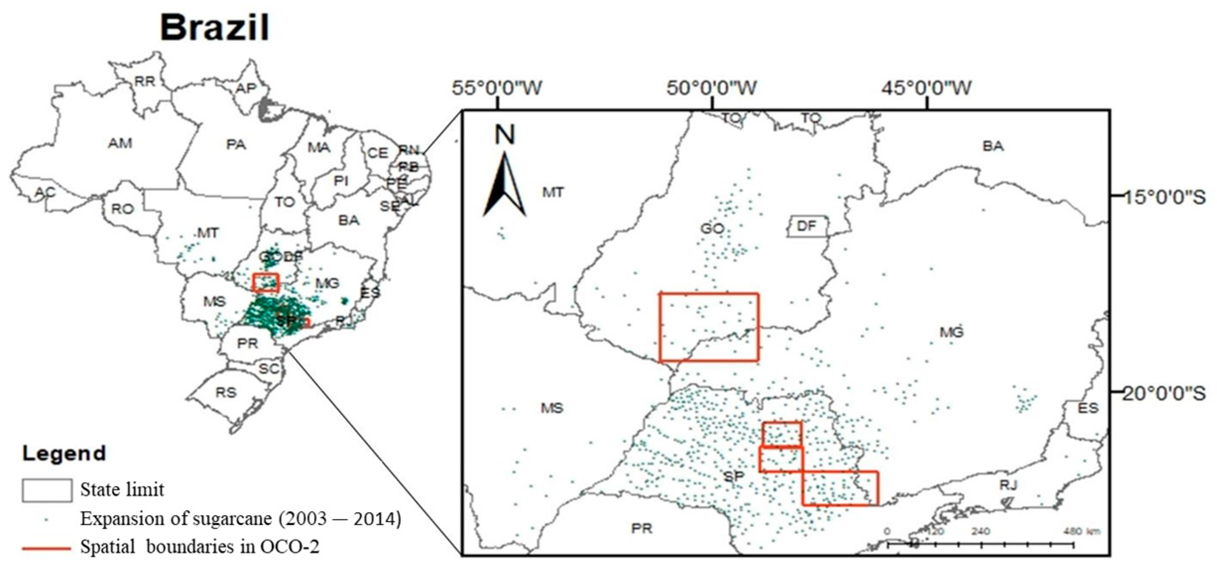
2.1. Description of Study Area

This study was conducted in four distinct locations chosen to represent the south-central region of Brazil (Figure 1): Pradópolis (21°21′ S latitude, 48°03′ W longitude; average altitude: 529 m), Araraquara (21°47′ S latitude, 48°10′ W longitude; average altitude: 664 m), and Iracemápolis (22°34′ S latitude, 47°31′ W longitude; average altitude: 608 m), all located within the state of São Paulo. Additionally, this study included Quirinópolis (18°26′ S latitude, 50°26′ W longitude; average altitude: 540 m), situated in the state of Goiás, Brazil.

These locations were selected to capture a diverse range of conditions relevant to sugarcane cultivation in the region. The state of São Paulo is renowned for hosting major sugarcane agroindustrial complexes in Brazil, particularly emphasizing sugar and bioenergy production. The cities of Pradópolis, Araraquara, and Iracemápolis are central to this agroindustrial activity, offering valuable insights into well-established sugarcane farming practices. Quirinópolis, located in Goiás, was included due to its recent expansion in sugarcane cultivation driven by national development plans, thus providing a contrast between traditional and expanding agricultural areas [31]. This selection of sites allows for a comprehensive analysis of the impact of different cultivation practices and regional developments on sugarcane yield.

According to Thornthwaite’s climate classification system [32], the localities were categorized as having a humid climate. Araraquara-SP, Iracemápolis-SP, Pradópolis-SP, and Quirinópolis-GO were classified as B1rB′4a, B1rB′3a, B1rA′a′, and B3rB′4a, respectively, under this system. The predominant soils of the localities were Ferric Acrisols in Iracemápolis-SP and Quirinópolis-GO, Humic Ferralsols in Araraquara-SP, and Humic Planosols in Pradópolis-SP [33] (WRB, 2015).

Ferric Acrisols are acidic, well-weathered soils typically found in tropical regions, characterized by a high content of iron oxides and low fertility. Humic Ferralsols, also found in tropical areas, are deeply weathered soils with high levels of iron and aluminum oxides, enriched with organic matter, which makes them more fertile compared to Ferric Acrisols. Humic Planosols are soils with a significant accumulation of organic matter in the top layer and are commonly found in flat areas prone to periodic flooding.

2.2. Satellite Data Products: Acquisition and Processing

The meteorological data spanning from 2015 to 2016 were obtained from orbital data systems (

Table 1. Variables of this study with sensors and platforms, temporal and spatial resolutions, and the measurement period.

Variable	Source	Temporal Resolution	Spatial Grid Resolution	Measurement Period
Average air temperature at 2 m (°C)	GEOS-5 FP-IT NASA/POWER [34]	Daily	1°	1 January 2013–31 December 2016
Global solar radiation (MJ m−2 d−1)	FLASHFlux Version 3 (A, B, C) NASA/POWER [34]	Daily	1°	1 January 2013–present
Precipitation (mm)	TRMM_3B42_Daily v7- NASA Giovanni [35]	Daily	0.25°	1 January 1998–present
NDVI [36]	(MOD13C2 v5) MODIS—Terra [37]	16-day	0.25°	1 February 2000–present
SIF 757 nm (W m−2 sr−1 µm−1)	OCO-2 [38]	16-day	1 km × 2 km	2 July 2014–present
xCO2 (ppm)	OCO-2 [38]	16-day	1 km × 2 km	2 July 2014–present
Wind speed at 10 m (m s−1)	GEOS-5 FP-IT NASA/POWER [34]	Daily	1°	1 January 2013– 31 December 2016
Relative humidity at 2 m (%)	GEOS-5 FP-IT NASA/POWER [34]	Daily	1°	1 January 2013– 31 December 2016

). These satellites and platforms have their own validation and quality control systems, which contribute to the accuracy and reliability of the data provided. This robust validation approach enhances the credibility of the meteorological analyses and ensures the precision of the obtained insights.

For meteorological analyses, daily data were adjusted on a monthly scale.

We utilized mean air temperature (T), global solar radiation (Qg), wind speed (u₂), and relative humidity (RH) to compute potential evapotranspiration (PET) using the Penman–Monteith method [39]. In this calculation, we considered the sensible heat flux on the ground to be equal to zero.

Soil water storage (STO, mm), water deficit (DEF, mm), and water excess (EXC, mm) were calculated at a 10-day interval, employing the Thornthwaite and Mather approach (Equations (1)–(6)). The assumed soil available water capacity (AWC) was defined as 100 mm.

$$if{(P-PET)}_i<0=\left\{\begin{array}{c}{NAC}_i={NAC}_{I-1}+{(P-PET)}_i\\ {STO}_i=AWC{e}^{{\displaystyle \frac{\left({NAC}_i\right)}{AWC}}}\end{array}\right.$$

(1)

$$if{(P-PET)}_i\ge 0=\left\{\begin{array}{c}{STO}_i={(P-PET)}_i+{STO}_{i-1}\\ {NAC}_i=AWC{ln}^{{\displaystyle \frac{\left({STO}_i\right)}{AWC}}}\end{array}\right.$$

(2)

$${ALT}_i={STO}_i-{STO}_{i-1}$$

(3)

$${AET}_i=\left\{\begin{array}{c}P+\left|{ALT}_i\right|,ifALT<0\\ {PET}_i,ifALT\ge 0\end{array}\right.$$

(4)

$$DEF=PET-AET$$

(5)

$${EXC}_i=\left\{\begin{array}{c}0,ifAWC<0\\ {(P-PET)}_i-{ALT}_i,ifAWC=0\end{array}\right.$$

(6)

where AWC = the available water capacity (in millimeters), denoting the maximum amount of water the soil can hold for plant use; STO = the soil water storage (in millimeters), indicating the current amount of water present in the soil; EXC = the water surplus within the soil-plant-atmosphere system (mm), indicating the excess water beyond the soil’s capacity; DEF = the water deficit of the soil-plant-atmosphere system (mm), representing the shortfall in water required by the soil-plant-atmosphere system, leading to diminished yield and changes in sugar content [40]; NAC = the negative difference between precipitation (P) and potential evapotranspiration (PET) values (mm), indicating a deficit situation where precipitation is less than potential evapotranspiration; P = precipitation (mm), denoting the amount of water that falls to the ground from the atmosphere; PET = potential evapotranspiration (mm), indicating the amount of water that could evaporate or transpire from a surface under optimal conditions; AET = actual evapotranspiration (mm), representing the real amount of water lost from the soil-plant-atmosphere system through evaporation and transpiration; ALT = the alteration in soil water storage between the current and previous months (mm), indicating the change in soil water content over time; and i = the current month under consideration in the analysis.

For annual agrometeorological data, we calculated the mean monthly air temperatures for each location. We accumulated monthly precipitation, water storage, water surplus, and water deficit on an annual scale.

The MODIS project features a spatial resolution that surpasses that of OCO-2. As a result, we collected NDVI data within the spatial confines outlined for OCO-2 (Table 1). Initially, we utilized the regression technique [41] to harmonize the trends in xCO₂ and SIF data.

We used the data on total recoverable sugars (TRS, kg t⁻¹) and tons of sugarcane per hectare (TCH) between April and November, during the 2015/2016 and 2016/2017 growing seasons.

Those data were collected by sugar mills routinely. Each truck arriving at the plant was weighed, and a sample was mechanically collected to determine the TRS. We gathered these monthly data from sugar mills of the region.

Considering the stalk density as one, the value of tons of sugarcane per hectare (TCH) was estimated according to Landell and Silva (2004) [42]. From the daily delivered loads, the sampling was collected by random selection among the possibilities at the mill. Subsequently, the calculation of the amount of total recoverable sugars (TRS) was performed [43].

The cultivation of sugarcane in the investigated regions can be classified into four distinct phenological phases: budburst, tillering, development, and maturation, in addition to the stages of planting and harvest [40]. Typically, planting occurs during the summer months, between February and March. In the first year of crop development, budburst usually happens between March and April. Tillering, characterized by the emergence of shoots from the plants, occurs from May to August, while the development phase typically spans from September to March of the second year (production year), followed by maturation from May to July. Harvesting typically begins in May and extends until August, depending on milling capacity. This average phenological information was gathered by Marcari et al. (2015) [40] over a period of more than 15 years in the same regions as this study.

2.3. Statistical Analysis

The assessment of the significance of each variable in the system was accomplished by employing multivariate analysis tools, specifically Principal Component Analysis (PCA), with standardized data (mean null and unit variance). PCA helps by transforming the original variables into a set of new variables called principal components. These components capture the most important patterns and relationships in the data. For example, in this study, PCA was used to identify which factors, such as climate variables, contribute most to variations in sugarcane yield. The new variables, or principal components, are created as linear combinations of the original variables based on their covariance [44]. The PCA was performed using Statistica 7.0 software [45].

We separated the data of SIF, xCO₂, and NDVI into quartiles, and we compared these to the sugarcane phenological phases. Response Surface Methods (RSM) were employed to investigate the relationships among TCH, TRS, SIF, xCO₂, and NDVI because RSM is particularly effective for exploring complex interactions between multiple variables and optimizing significant parameters. In our study, these methods were chosen due to their ability to model and analyze the influence of various factors on sugarcane productivity and quality, enabling us to identify optimal levels for these responses. RSM helps in understanding how different combinations of TCH, TRS, SIF, xCO₂, and NDVI affect sugarcane outcomes, which is crucial for making informed decisions in agricultural management [46]. We created the response surface graphics using Table Curve 3D 4.0 software (Systat Software Incorporated, San Jose, CA, USA).

To evaluate the associations between variables, we utilize several indices: (1) Pearson correlation (r); (2) adjusted coefficient of determination (R² adj); (3) Mean Absolute Percentage Error (MAPE); and (4) Root Mean Square Error (RMSE). These indices, expressed through Equations (7)–(10), enable a comprehensive assessment of the relationships under consideration.

$$r={\displaystyle \frac{\sum _{i=1}^n({Yobs}_i-\overline{Yobs})\times ({Yest}_i-\overline{Yest})}{\sqrt{\sum _{i=1}^n{({Yobs}_i-\overline{Yobs})}^2}\times \sqrt{\sum _{i=1}^n{({Yest}_i-\overline{Yest})}^2}}}$$

(7)

$$R^{2}adj=\left[1-{\displaystyle \frac{(1-R^2)\times (n-1)}{N-k-1}}\right]$$

(8)

$$MAPE\left(\%\right)={\displaystyle \frac{\sum _{i=1}^n\left(\right|\frac{{Yest}_i-{Yobs}_i}{{Yest}_i}|\times 100)}{N}}$$

(9)

$$RMSE=\sqrt{{\displaystyle \frac{\sum _{i=1}^N{(Yobs}_i-{Yest}_i)}{N}}}$$

(10)

where ${Yest}_i$: estimated value; ${Yobs}_i$: observed value; $N$: number of data; and $k$: number of independent variables in the regression.

3. Results

The mean annual temperature in the surveyed areas was 23 °C (Figure 2), with Iracemápolis-SP experiencing the lowest recorded annual temperature at 22 °C and Quirinópolis-GO recording the highest at 25 °C. Notably, Araraquara-SP and Pradópolis-SP both maintained a mean air temperature of 23 °C during the 2015–2016 period.

The annual precipitation recorded for Araraquara, Iracemápolis, Pradópolis, and Quirinópolis was 1498 mm, 1923 mm, 1652 mm, and 1344 mm, respectively (Figure 2). In 2015, all locations experienced one of the rainiest periods, but there was an average 88% reduction in precipitation during the winter months (June to September) compared to 2016.

The average annual EXC across the regions was 806 mm, reaching its peak soil water storage occurring in January and March, as shown in Figure 3, aligning with the sugarcane planting and high growth phases. Iracemápolis exhibited the highest EXC (1289 mm), whereas Quirinópolis had the lowest at 378 mm. Water deficits followed this order: Quirinópolis-GO (1379 mm), Pradópolis-SP (750 mm), Araraquara-SP (694 mm), and Iracemápolis-SP (453 mm), as shown in Figure 3. In 2016, Araraquara-SP, Pradópolis-SP, and Quirinópolis-GO experienced more significant water deficits compared to 2015.

During 2015 and 2016, the average value of TCH was 82.8 t ha⁻¹, while TRS was 128 kg t⁻¹, with seasonal variations (Figure 4). In April, the annual production cycle is initiated, characterized by high TCH and relatively low TRS values. This production phase typically extends on average until November. There was a monthly decrease of 1.18 t ha⁻¹ in TCH and an increase of 2.75 kg t⁻¹ in TRS from April to November. Iracemápolis recorded the highest average TCH at 89 t ha⁻¹, with the lowest TRS value at 125 kg t⁻¹ (Figure 5b). Quirinópolis, on the other hand, had the highest TRS value at 133 kg t⁻¹ (Figure 5d).

Principal Component Analysis (PCA) explained 62% of the total variability, utilizing the first two principal components. PC1 accounted for 38% of the total variance in the sugarcane crop, while PC2 explained 23% of the original data’s total variance (Figure 6). TRS exhibited higher sensitivity than TCH under the studied conditions, directly responding to xCO₂ and water deficit (DEF) and inversely to SIF and NDVI (Figure 6). TRS showed a direct correlation with DEF and T and an inverse correlation with P and EXC. TCH correlated with all variables, directly to P, EXC, SIF, and NDVI, and indirectly to DEF, T, TRS, and xCO₂. Seasonal variations in SIF, NDVI, and xCO₂ were similar in the two years studied (Figure 7). Negative linear correlations were observed between SIF and xCO₂ (r = −0.69, p < 0.05) and between xCO₂ and NDVI (r = −0.49, p < 0.05) during the cane cycle. In contrast, a positive correlation was observed between SIF and NDVI (r = 0.55, p < 0.05). Average SIF and NDVI decreased, while xCO₂ increased between June and mid-September, corresponding to winter, with minimum values for SIF and NDVI around 0.5 W m⁻² sr⁻¹ μm⁻¹ and 0.45, respectively (Figure 7). Between October and February, there was an increase in values of SIF and NDVI and a decrease in xCO₂, with the highest SIF and NDVI values at 1.6 W m⁻² sr⁻¹ μm⁻¹ and 0.7, respectively.

We established value ranges for SIF, xCO₂, and NDVI based on quartiles (

Table 2. Different conditions based on quartiles of Solar-Induced Chlorophyll Fluorescence (SIF), column-averaged CO₂ (xCO₂) and Normalized Difference Vegetation Index (NDVI) about the development of sugarcane.

Classification	SIF (W m−2 sr−1 µm−1)	xCO2 (ppm)	NDVI
High	x > 0.7	x > 412.5	x > 0.5
Medium	0.4 ≤ x ≤ 0.7	411.5 ≤ x ≤ 412.5	0.4 ≤ x ≤ 0.5
Low	x < 0.4	x < 411.5	x < 0.4

) and correlated these with each phenological phase (

Table 3. Conditions of the crop in relation to SIF, xCO₂, and NDVI in localities of this study.

Condition
I		II	III	IV	V
	Beginning Development	Middle Development	Beginning Maturation	Middle Maturation	End of harvest
SIF	High	Medium	Low	Low	Medium
xCO2	Low	Low	Medium	High	Medium
NDVI	Low	High	High	Medium	Low

). These criteria were applied to each main phenological phase of sugarcane, considering the unique conditions of each phase. For example, SIF, xCO₂, and NDVI were analyzed in relation to the onset of sugarcane maturation, distinguishing their low (<0.4 W m⁻² sr⁻¹ µm⁻¹), medium (411.5 ppm ≤ xCO₂ ≤ 412.5 ppm), and high (>0.5 W m⁻² sr⁻¹ µm⁻¹) values, respectively. It is important to note that sprouted sugarcane (<20% of the area) could introduce some error into these criteria.

Regional values of SIF, NDVI, and xCO₂ exhibited variations among regions. SIF showed the highest coefficient of variation (CV) at the monthly scale, reaching 52% among the localities, while NDVI and xCO₂ had CVs of 34% and 0.37%, respectively (Figure 8). The months of greatest variability occurred in the second half of the year. SIF for all localities peaked at values of xCO₂ less than 400 ppm and NDVI between 0.4 and 0.7. The adjusted quadratic model was SIF = −4.8405NDVI² − 0.0169 xCO₂² − 48.3371NDVI + 13.413 xCO₂ + 0.1323NDVI xCO₂ − 2661.9698, with a Mean Absolute Percentage Error (MAPE) of 0.25% (Figure 9).

Adjustments were made for TCH and TRS as functions of SIF, NDVI, and xCO2. All response surfaces were significant at the 0.05 level (Figure 10). The models demonstrated high accuracy with MAPEs below 8.54%. TRS decreased when SIF values were between 0.4 W m⁻² sr⁻¹ μm⁻¹ and 0.8 W m⁻² sr⁻¹ μm⁻¹, and NDVI less than 0.5. TRS values maximized at 15 kg t⁻¹ with low NDVI and XCO₂, coupled with smaller SIFs of 0.4 W m⁻² sr⁻¹ μm⁻¹ and greater than 1 W m⁻² sr⁻¹ μm⁻¹ (Figure 11B,D,F). The relationships of SIF, xCO₂, and NDVI with TCH and TSR are illustrated in Figure 11. The adjusted models explained 2%, 17%, and 33% of the mean variation of TCH. The SIF model demonstrated the best accuracy performance for TCH data (RMSE = 82,970 t ha⁻¹) (Figure 11A). The models using SIF and NDVI showed similar RMSE values.

4. Discussion

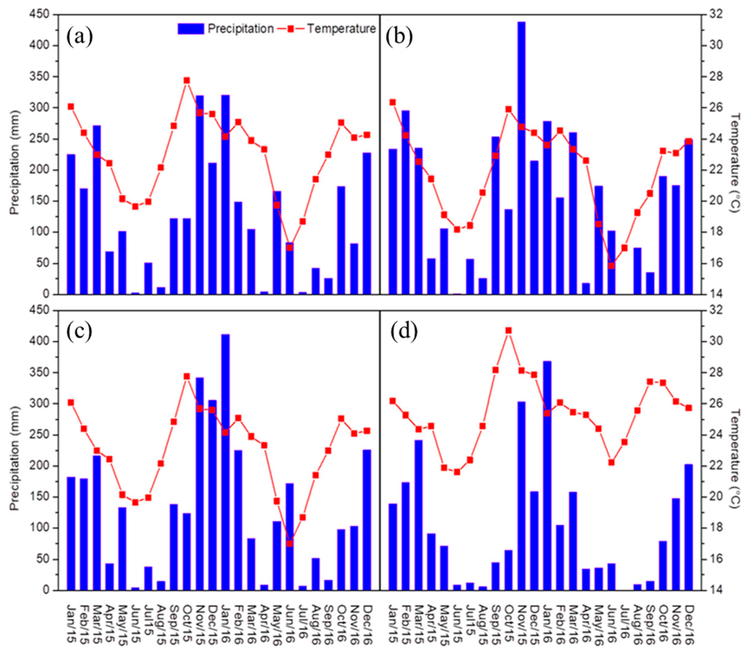
4.1. Air Temperature and Precipitation

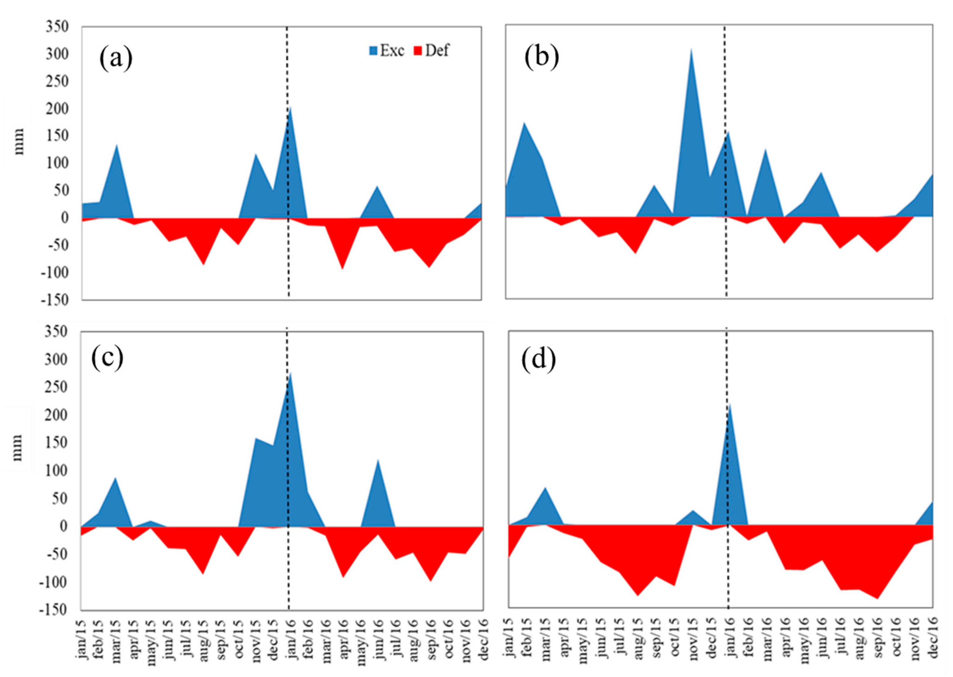
The localities experience air temperatures suitable for the growth and sugar accumulation in sugarcane, as temperatures ranging from 18 °C to 38 °C are known to be favorable for sugarcane cultivation [47]. Air temperature significantly influences evapotranspiration and water use efficiency, with water availability playing a crucial role in regulating these factors in tropical sugarcane production [48] (Da Silva et al., 2013).

The average annual p values observed in this study fall within the range of sugarcane’s water requirements. With 1000 mm of precipitation, evenly distributed spatially, it proves sufficient to support high yields without the need for additional irrigation [49].

During the winter months, both temperature and precipitation decrease, coinciding with key stages in sugarcane growth, such as tillering, the initiation of vegetative development, maturation, and harvesting. The lower air temperatures during this period are advantageous for sucrose concentration, as they tend to limit plant growth [50].

4.2. Hydric Balance

Sprouting and vegetative development take place during the spring and summer, specifically from October to March. The analyzed period exhibited favorable conditions with sufficient water surplus and appropriate air temperatures (Figure 2). In south-central Brazil, sugarcane crops show a heightened demand for air temperature, water, and solar radiation in October and March, aligning with the tillering and more intensive vegetative growth stages occurring between 60 and 150 days after planting [51].

Water deficit has a detrimental impact on photosynthesis, which is a primary factor in reducing both growth and yield of sugarcane [52,53]. In winter, the stages of tillering and the commencement of vegetative development experience more pronounced water deficiency. Under these water-limiting conditions, sugarcane’s primary response involves the closure of stomata to prevent water loss through leaf transpiration. Consequently, this plant reaction restricts the availability of CO₂ for photosynthesis, leading to the inhibition of biomass production. Additionally, there is a reduction in chlorophyll content in the leaves [54].

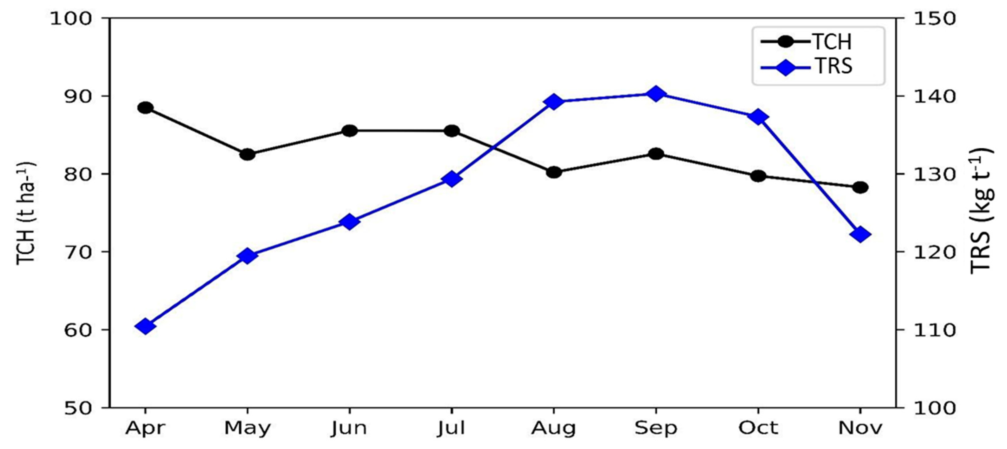
4.3. Sugarcane Yield and Quality

The sugarcane harvest season is intricately connected to the chosen planting system, which can either be a one-year or a one-year-and-a-half system, thereby impacting yield. Months during the harvest characterized by higher total recoverable sugars (TRS) values and lower tons of sugarcane per hectare (TCH) values are closely associated with the significance of soil water reduction and temperature decline during the crop’s maturation stage. The increase in sucrose content in the stalks prompts maturation, with the potential occurrence of the maximum sucrose point at this stage [55]. Typically, the harvest commences in April, marked by reduced vegetative growth, and may extend through November.

The reduction in TCH and the elevation in TRS are linked to an extended period of drought between April and November, which restricts biomass accumulation due to low soil moisture during autumn and winter. This leads to stomatal closure, resulting in decreased photosynthesis rates [56]. The suspension of sugarcane growth due to water deficiency promotes sugar concentration. This period encompasses the final stage of vegetative growth, the maturation phase, and the initiation of the crop’s tillering period. The E, F values of Solar-Induced Fluorescence (SIF), Normalized Difference Vegetation Index (NDVI), and xCO₂ are markedly influenced by the extent of sugarcane cultivation in the region, which aligns with the findings discussed by [57].

4.4. Principal Component Analysis

PC1 is associated with meteorological and water conditions, while PC2 is linked to vegetation indices. The collective examination of climatic conditions, water balance, tons of sugarcane per hectare (TCH), and total recoverable sugars (TRS) by principal components indicates that TCH is influenced by the combined impact of all these elements. Our findings align with those of Da Silva et al. (2013) [48], who highlighted the influence of mean air temperature (T) on the direct relationship between development and production.

The findings of this study reveal that sugarcane productivity, as measured by TCH and TRS, is strongly influenced by the interaction between meteorological conditions, water balance, and vegetation indices. This highlights the need for an integrated approach to agricultural management, combining detailed climate forecasts with continuous monitoring of water and vegetation conditions. Adjusting cultivation practices based on this information can optimize production and resource use efficiency, promoting more sustainable agriculture. Additionally, the results of this study could serve as a foundation for public policies that encourage adaptive and sustainable agricultural practices. To deepen the understanding of these complex relationships, future research could include a more comprehensive analysis of climatic and water variables across different seasonal cycles and regions. Longitudinal studies and integrated economic modeling could provide further insights into the feasibility and economic benefits of the recommended practices. This approach would not only enhance sugarcane productivity but also contribute to more effective resource management strategies and adaptation to climate change.

Precipitation (P) primarily affects tillering, creating potential for later TRS accumulation during maturation [16]. TRS exhibits a direct correlation with water deficiency (DEF) during maturation. There exists a direct relationship between temperature (T) and precipitation (P) with TCH. The high-intensity vegetative growth of the crop, typically occurring from October to March, results in the accumulation of approximately 75% of plant mass, necessitating favorable precipitation, air temperature, and radiation [40].

The similarity in seasonal variation indicates a relationship between vegetation indexes and the productive management of sugarcane, in addition to the climatic conditions in the south-central region of Brazil. TCH shows a direct correlation with Solar-Induced Fluorescence (SIF) and Normalized Difference Vegetation Index (NDVI) and an inverse correlation with xCO₂ (PC1, Figure 6). SIF reflects the photosynthetic process that supports the growth and development of the crop. The decrease in xCO₂ signifies the absorption of atmospheric CO₂ by the crop, showcasing the efficiency of photosynthesis in sugarcane growth, consequently increasing TCH. NDVI is associated with the biomass of these crops. The inverse relationship of TCH with xCO₂ is likely due to the expansion of the photosynthetic area. As a result, the absorption of atmospheric CO₂ occurs for TCH production, leading to an increase in TCH and a decrease in xCO₂. TRS is directly correlated with xCO₂ and inversely correlated with SIF and NDVI. These findings provide new insights into the existing literature. While studies often link yield and sugar levels with NDVI in sugarcane [11,58,59], no work has been identified regarding sugarcane crops and the estimation of Gross Primary Productivity (GPP) using vegetation indexes such as NDVI and SIF measured by satellites [59].

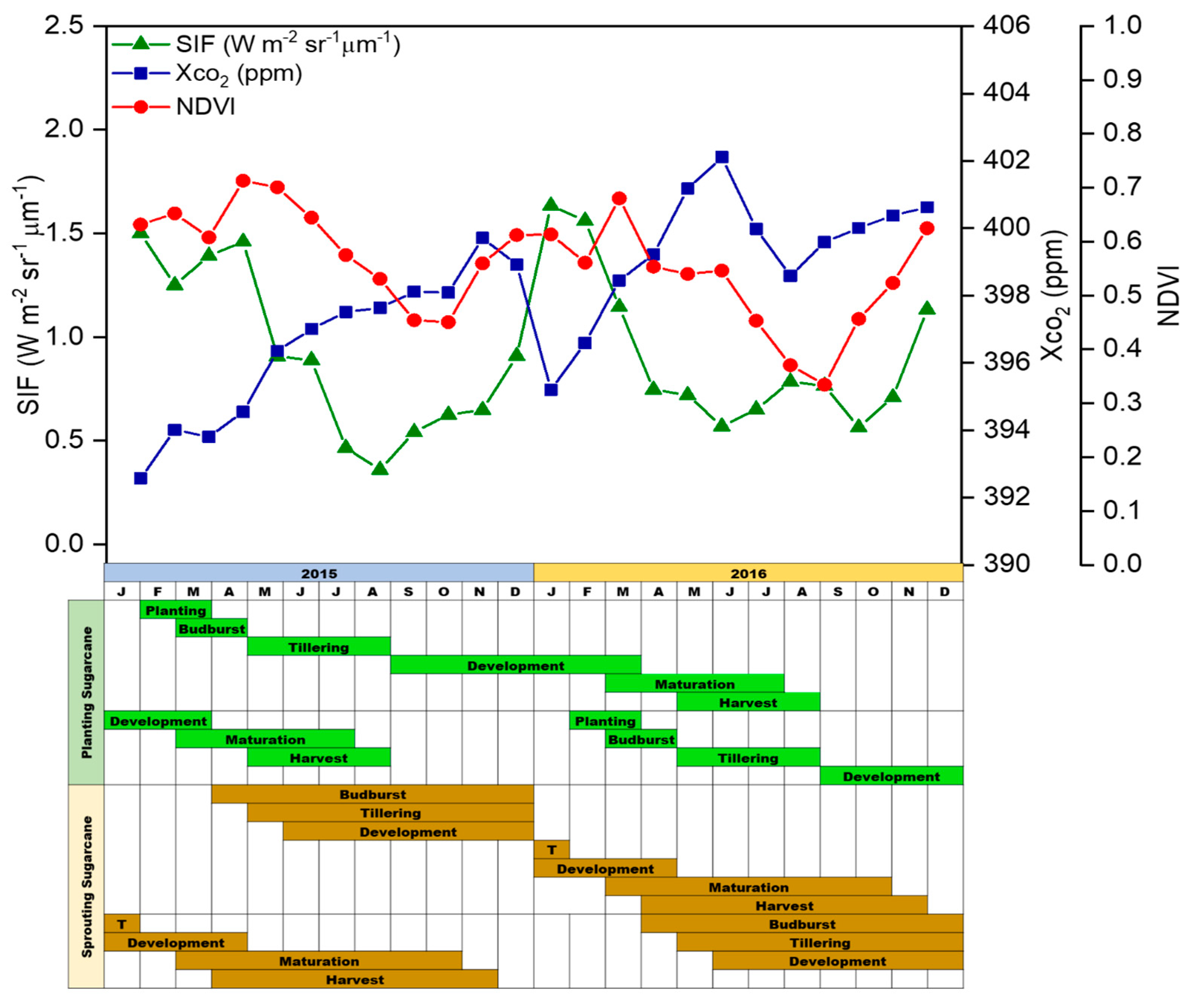
4.5. SIF, xCO₂, and NDVI

Solar-Induced Fluorescence (SIF) is produced during photosynthesis and is strongly correlated with agricultural production [21]. The Normalized Difference Vegetation Index (NDVI) is associated with vegetative vigor, leaf area index, and canopy biomass [59]. In contrast, xCO₂ relates to the fixation of CO₂ by the crop resulting from photosynthesis (Figure 6).

A study by Wei et al. (2019) [60] found that satellite-based SIF outperforms NDVI in estimating autumn harvest production in China. SIF is more effective than traditional vegetation indices for monitoring crop dynamics. The notable negative relationships between SIF and xCO₂, and between xCO₂ and NDVI, indicate increased photosynthetic activity and biomass production, which leads to a reduction in atmospheric CO₂ captured and fixed by plants (Figure 7). The strong positive relationship between SIF and NDVI reflects an increase in biomass associated with photosynthesis in agricultural areas.

Although OCO-2 SIF products have lower spatial resolutions compared to MODIS variables (≤1 km), Peng et al. (2020) [61] observed that SIF data is effective for crop yield forecasting. Our study identified seasonal patterns of SIF, NDVI, and xCO₂ during different phenological phases of sugarcane (Figure 7). However, higher spatial resolution in SIF data would improve differentiation between crops like maize and soybean, as noted by Peng et al. Moreover, between January and April, new sugarcane areas are planted while the previous year’s plots undergo development and early maturation. The period of sprouted sugarcane coincides with tillering and crop development in the region, resulting in increased SIF and NDVI and decreased xCO₂ (Figure 7).

The decline in SIF and NDVI during winter corresponds to tillering in sugarcane and the final stages of maturation and harvesting in sugarcane regions (Figure 7). From October to February, the increase in SIF and NDVI reflects the development and maturation/harvest of planted and sprouted sugarcane in the studied regions, respectively. The coefficient of variation (CV) of these variables across different localities shows significant variability between years, revealing distinct patterns between months (Figure 8). This variability allows for a detailed analysis of the phenological stages of the crop.

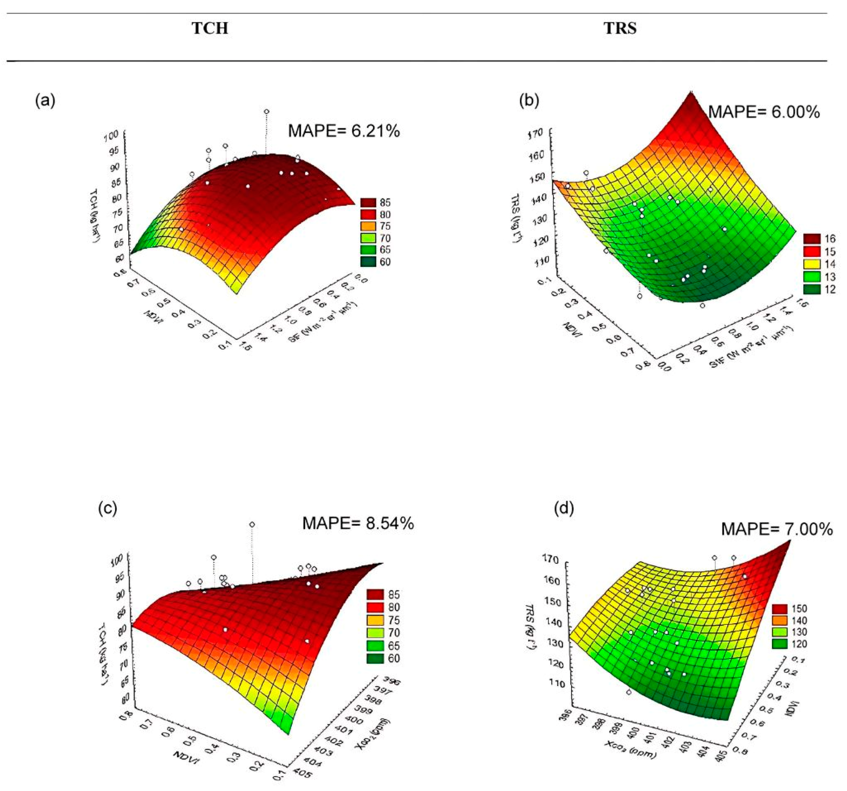
4.6. Response Surface

The adjustments made to the response surfaces aimed to establish a detailed relationship between Solar-Induced Fluorescence (SIF), Normalized Difference Vegetation Index (NDVI), and xCO₂ and their correlation with tons of sugarcane per hectare (TCH) and total recoverable sugars (TRS) across all localities (Figure 10). The maximum TCH, approximately 95 t ha⁻¹, was observed when NDVI and SIF values were lower (Figure 11A,C,E).

In a study by Peng et al. (2020) [61], it was found that high-resolution SIF products from OCO-2 and TROPOMI outperformed the use of coarse-resolution SIF products from GOME-2 in forecasting corn and soybean yields in the USA.

The simultaneous increase in TRS with high SIF values is linked to the tillering period (Figure 11B,D,F). The decline in NDVI and SIF values is likely associated with leaf senescence, particularly after flowering, and is correlated with an increase in TRS during the maturation period. Mean Absolute Percentage Error (MAPE) values below 9% are considered appropriate for crop yield estimation models using remote sensing data as independent variables [40,62,63]. Despite this study’s limitations, such as the moderate spatial resolution of independent variables and the yield and sugar level data, as well as the use of only one remote sensing variable for each model (Figure 11), these findings are promising.

4.7. Practical Implications and Future Research Directions

The findings of this study underscore the value of integrating climatic, hydric, and vegetation indices to optimize sugarcane production. The results suggest that combining data on Solar-Induced Fluorescence (SIF), Normalized Difference Vegetation Index (NDVI), and column-averaged CO₂ (xCO₂) can significantly enhance agricultural management and decision-making for sugarcane cultivation. Practically, this implies that agricultural practices should be adjusted based on these indices to optimize irrigation, soil management, and harvest timing. Implementing such information can lead to more sustainable agriculture by maximizing yield and quality while adapting to climatic and hydric variability.

For future research, we recommend conducting longitudinal studies that explore climatic and hydric variables across different seasonal cycles and regions. Incorporating integrated economic modeling could provide valuable insights into the feasibility and economic benefits of the proposed practices. Additionally, utilizing higher spatial resolution data, particularly for SIF, could improve accuracy in yield forecasting and differentiation between crop types. Such approaches would not only enhance the understanding of the complex relationships between climate, water, and sugarcane productivity but also contribute to more effective resource management strategies and adaptation to climate change.

5. Conclusions

This study provides significant evidence of the relationship between column-averaged CO₂ (xCO₂), Solar-Induced Chlorophyll Fluorescence (SIF), Normalized Difference Vegetation Index (NDVI), and the sugar yield and quality of sugarcane. The increase in SIF indicates the vegetative growth of sugarcane, while high xCO₂ values suggest the establishment and harvest stages, and high NDVI values signify crop maturation.

The results show that total recoverable sugar (TRS) is more sensitive to SIF, NDVI, xCO₂, and agrometeorological variables compared to tonnage of sugarcane per hectare (TCH). Specifically, TRS exhibited a direct relationship with xCO₂, DEF (an indicator of crop defense mechanisms), and temperature (T), while an inverse relationship was observed with SIF, NDVI, precipitation (P), and evapotranspiration (EXC). On the other hand, TCH demonstrated a direct relationship with NDVI, SIF, EXC, and P and an inverse relationship with xCO₂, T, and DEF.

The robust relationship established in this study lays a solid foundation for further research and the development of practical applications that leverage SIF, xCO₂, and NDVI data to optimize sugarcane production and enhance decision-making in the agricultural sector. These findings highlight the importance of integrating various indices and variables for more efficient and productive crop management.

References

1. La Scala Junior, N.; De Figueiredo, E.; Panosso, A. A review on soil carbon accumulation due to the management change of major Brazilian agricultural activities. Braz. J. Biol. 2012, 72, 775–785. [Google Scholar] [CrossRef] [PubMed]
2. Bordonal, R.O.; Tenelli, S.; Oliveira, D.M.S.; Chagas, M.F.; Cherubin, M.R.; Weiler, D.A.; Campbell, E.; Gonzaga, L.C.; Barbosa, L.C.; Cerri, C.E.P.; et al. Carbon savings from sugarcane straw-derived bioenergy: Insights from a life cycle perspective incluing soil carbono changes. Sci. Total Environ. 2024, 947, 174670. [Google Scholar] [CrossRef] [PubMed]
3. Wang, Y.; Yuan, Q.; Li, T.; Yang, Y.; Zhou, S.; Zhang, L. Seamless mapping of long-term (2010–2020) daily global XCO2 and XCH4 from the Greenhouse Gases Observing Satellite (GOSAT), Orbiting Carbon Observatory 2 (OCO-2), and CAMS global greenhouse gas reanalysis (CAMS-EGG4) with a spatiotemporally self-supervised fusion method. Earth Syst. Sci. Data 2023, 15, 3597–3622. [Google Scholar] [CrossRef]
4. Santos, G.A.A.; Silva, F.F.; Águas, T.A.; Meneses, K.C.; Costa, L.M.; Silva Junior, C.A.; Rolim, G.S.; La Scala, N., Jr. Temporal and Spatial Patterns of XCO2 and SIF as observed by OCO-2: A case study in the Midwest region of Brazil. J. Indian Soc. Remote Sens. 2024. [Google Scholar] [CrossRef]
5. Aparecido, L.E.O.; Torsoni, G.B.; Lorençone, J.A.; Lorençone, P.A.; Lima, R.F.; Rolim, G.S.; Saqui, D.; Oliveira Junior, G.G. Future climate suitability of Hemileia vastatrix in arabica coffee under CMIP6 scenarios. J. Sci. Food Agric. 2024. [Google Scholar] [CrossRef]
6. Silva, L.L.D.; Costa, R.F.D.; Campos, J.H.D.C.; Dantas, R.T. Influence of precipitations on agricultural productivity in Paraíba State. Rev. Bras. De Eng. Agrícola E Ambient. 2009, 13, 454–461. [Google Scholar] [CrossRef]
7. Jensen, R.; Herbst, M.; Friborg, T. Direct and indirect controls of the interannual variability in atmospheric CO2 exchange of three contrasting ecosystems in Denmark. Agric. For. Meteorol. 2017, 233, 12–31. [Google Scholar] [CrossRef]
8. Yu, D.; Zha, Y.; Shi, L.; Jin, X.; Hu, S.; Yang, Q.; Huang, K.; Zeng, W. Improvement of sugarcane yield estimation by assimilating UAV-derived plant height observations. Eur. J. Agron. 2020, 121, 126159. [Google Scholar] [CrossRef]
9. Rahman, M.M.; Robson, A.J. A novel approach for sugarcane yield prediction using landsat time series imagery: A case study on Bundaberg region. Adv. Remote Sens. 2016, 5, 93–102. [Google Scholar] [CrossRef]
10. Rahman, M.M.; Robson, A. Integrating landsat-8 and sentinel-2 time series data for yield prediction of sugarcane crops at the block level. Remote Sens. 2020, 12, 1313. [Google Scholar] [CrossRef]
11. Fernandes, J.L.; Ebecken, N.F.F.; Esquerdo, J.C.D.M. Sugarcane yield prediction in Brazil using NDVI time series and neural networks ensemble. Int. J. Remote Sens. 2017, 38, 4631–4644. [Google Scholar] [CrossRef]
12. Krause, G.H.; Weis, E. Chlorophyll Fluorescence and Photosynthesis: The Basics. Annu. Rev. Plant Physiol. Plant Mol. Biol. 1991, 42, 313–349. [Google Scholar] [CrossRef]
13. De Araújo Santos, G.A.; Morais Filho, L.F.F.; de Meneses, K.C.; da Silva Junior, C.A.; de Souza Rolim, G.; La Scala, N., Jr. Hot spots and anomalies of CO2 over eastern Amazonia, Brazil: A time series from 2015 to 2018. Environ. Res. 2022, 215, 114379. [Google Scholar] [CrossRef] [PubMed]
14. Da Costa, L.M.; de Araújo Santos, G.A.; Panosso, A.R.; de Souza Rolim, G.; La Scala, N. An empirical model for estimating daily atmospheric column-averaged CO2 concentration above São Paulo state, Brazil. Carbon Balance Manag. 2022, 17, 9. [Google Scholar] [CrossRef] [PubMed]
15. Guan, K.; Wu, J.; Kimball, J.S.; Anderson, M.C.; Frolking, S.; Li, B.; Hain, C.R.; Lobell, D.B. The shared and unique values of optical, fluorescence, thermal and microwave satellite data for estimating large-scale crop yields. Remote Sens. Environ. 2017, 199, 333–349. [Google Scholar] [CrossRef]
16. Verma, M.; Schimel, D.; Evans, B.; Frankenberg, C.; Beringer, J.; Drewry, D.T.; Magney, T.; Marang, I.; Hutley, L.; Moore, C.; et al. Effect of environmental conditions on the relationship between solar-induced fluorescence and gross primary productivity at an OzFlux grassland site. J. Geophys. Res. Biogeosci. 2017, 122, 716–733. [Google Scholar] [CrossRef]
17. Frankenberg, C.; Berry, J.; Guanter, L.; Joiner, J. Remote sensing of terrestrial chlorophyll fluorescence from space. SPIE Newsroom 2013, 19, 4725. [Google Scholar] [CrossRef]
18. Doughty, R.; Kurosu, T.P.; Parazoo, N.; Köhler, P.; Wang, Y.; Sun, Y.; Frankenberg, C. Global GOSAT, OCO-2, and OCO-3 solar-induced chlorophyll fluorescence datasets. Earth Syst. Sci. Data 2022, 14, 1513–1529. [Google Scholar] [CrossRef]
19. Meroni, M.; Rossini, M.; Guanter, L.; Alonso, L.; Rascher, U.; Colombo, R.; Moreno, J. Remote sensing of solar-induced chlorophyll fluorescence: Review of methods and applications. Remote Sens. Environ. 2009, 113, 2037–2051. [Google Scholar] [CrossRef]
20. Zarco-Tejada, P.J.; Gonzalez-Dugo, V.; Williams, L.E.; Suárez, L.; Berni, J.A.J.; Goldhamer, D.; Fereres, E. A PRI-based water stress index combining structural and chlorophyll effects: Assessment using diurnal narrow-band airborne imagery and the CWSI thermal index. Remote Sens. Environ. 2013, 138, 38–50. [Google Scholar] [CrossRef]
21. Li, X.; Xiao, J.; He, B.; Arain, M.A.; Beringer, J.; Desai, A.R.; Emmel, C.; Hollinger, D.Y.; Krasnova, A.; Mammarella, I.; et al. Solar-induced chlorophyll fluorescence is strongly correlated with terrestrial photosynthesis for a wide variety of biomes: First global analysis based on OCO-2 and flux tower observations. Glob. Chang. Biol. 2018, 24, 3990–4008. [Google Scholar] [CrossRef] [PubMed]
22. Wang, S.; Zhang, L.; Huang, C.; Qiao, N. An NDVI-based vegetation phenology is improved to be more consistent with photosynthesis dynamics through applying a light use efficiency model over boreal high-latitude forests. Remote Sens. 2017, 9, 695. [Google Scholar] [CrossRef]
23. Singh, P.; Kikon, N.; Verma, P. Impact of land use change and urbanization on urban heat island in Lucknow city, Central India. A remote sensing based estimate. Sustain. Cities Soc. 2017, 32, 100–114. [Google Scholar] [CrossRef]
24. Clerici, N.; Weissteiner, C.J.; Gerard, F. Exploring the use of MODIS NDVI-based phenology indicators for classifying forest general habitat categories. Remote Sens. 2012, 4, 1781–1803. [Google Scholar] [CrossRef]
25. Rao, P.V.K.; Rao, V.V.; Venkataratnam, L. Remote sensing: A technology for assessment of sugarcane crop acreage and yield. Sugar Tech 2002, 4, 97–101. [Google Scholar] [CrossRef]
26. Somkuti, P.; Bösch, H.; Feng, L.; Palmer, P.I.; Parker, R.J.; Quaife, T. A new space-borne perspective of crop productivity variations over the US Corn Belt. Agric. For. Meteorol. 2020, 281, 107826. [Google Scholar] [CrossRef]
27. Merrick, T.; Pau, S.; Jorge, M.L.S.; Silva, T.S.F.; Bennartz, R. Spatiotemporal patterns and phenology of tropical vegetation solar-induced chlorophyll fluorescence across Brazilian biomes using satellite observations. Remote Sens. 2019, 11, 1746. [Google Scholar] [CrossRef]
28. Shekhar, A.; Chen, J.; Paetzold, J.C.; Dietrich, F.; Zhao, X.; Bhattacharjee, S.; Ruisinger, V.; Wofsy, S.C. Anthropogenic CO2 emissions assessment of Nile Delta using XCO2 and SIF data from OCO-2 satellite. Environ. Res. Lett. 2020, 15, 095010. [Google Scholar] [CrossRef]
29. Dass, A.; Mishra, A.K.; Santos, G.A.A.; Ranjan, R.K. Spatio-temporal variation of atmospheric CO2 and its association with anthropogenic, vegetation, and climate indices over the state of Bihar, India. Environ. Adv. 2024, 16, 100513. [Google Scholar] [CrossRef]
30. Qiu, R.; Han, G.; Ma, X.; Sha, Z.; Shi, T.; Xu, H.; Zhang, M. CO2 concentration, a critical factor influencing the relationship between solar-induced chlorophyll fluorescence and gross primary productivity. Remote Sens. 2020, 12, 1377. [Google Scholar] [CrossRef]
31. Oliveira, A.D.; Ramalho, J. Plano Nacional de Agroenergia 2006–2011; Ministério da Agricultura, Pecuária e Abastecimento. Embrapa Informação Tecnológica: Brasilia, Brasil, 2006; 114p. [Google Scholar]
32. Thornthwaite, C.W. An approach toward a rational classification of climate. Geogr. Rev. 1948, 38, 55–94. [Google Scholar] [CrossRef]
33. World Reference Base for Soil Resources. Update 2015: International Soil Classification System for Naming Soils and Creating Legends for Soil Maps; International Union of Soil Sciences (IUSS): Rome, Italy, 2014. [Google Scholar]
34. Stackhouse, P.W.; Westberg, D.; Chandler, W.S.; Zhang, T.; Hoell, J.M. Prediction of Worldwide Energy Resource (POWER)—Agroclimatology Methodology—(1.0 Latitude by 1.0 O Longitude Spatial Resolution). 2017. Available online: https://power.larc.nasa.gov/docs/ (accessed on 11 November 2019).
35. NASA Giovanni. Available online: https://giovanni.gsfc.nasa.gov/giovanni/ (accessed on 16 September 2024).
36. Rouse, J.W.; Haas, R.H.; Schell, J.A.; Deering, D.W. Monitoring vegetation systems in the Great Plains with ERTS. NASA Spec. Publ 1974, 351, 309. [Google Scholar]
37. Embrapa. “Sistema de Análise Temporal da VegetaçãoSATVeg”. Campinas. 2018. Available online: www.satveg.cnptia.embrapa.br/satveg/login.html (accessed on 11 November 2019).
38. Crisp, D.; Fisher, B.M.; O’Dell, C.; Frankenberg, C.; Basilio, R.; Bösch, H.; Brown, L.R.; Castano, R.; Connor, B.; Deutscher, N.M.; et al. The ACOS CO2 retrieval algorithm—Part II: Global XCO2 data characterization. Atmos. Meas. Tech. 2012, 5, 687–707. [Google Scholar] [CrossRef]
39. Allen, R.G.; Pereira, L.S.; Raes, D.; Smith, M.; Ab, W. Allen; FAO: Rome, Italy, 1998; pp. 1–15. [Google Scholar]
40. Marcari, M.A.; de Souza Rolim, G.; de Oliveira Aparecido, L.E. Agrometeorological models for forecasting yield and quality of sugarcane. Aust. J. Crop Sci. 2015, 9, 1049–1056. [Google Scholar]
41. Gujarati, D.N.; Porter, D.C. Econometria Básica, 5th ed.; Amgh Editora: Belo Horizonte, Brazil, 2011. [Google Scholar]
42. Landell, M.D.A.; Silva, M.D.A. As estratégias de seleção da cana em desenvolvimento no Brasil. Visão Agrícola 2004, 1, 18–23. [Google Scholar]
43. Marques, T.A.; Neves, L.C.G.; Rampazo, E.M.; Junior, E.L.D.; Souza, F.C.; Marques, P.A.A. TRS value of sugarcane according to bioenergy and sugar levels. Acta Sci. Agron. 2015, 37, 347–353. [Google Scholar] [CrossRef]
44. Hair, J.F.; Black, W.C.; Babin, B.J.; Anderson, R.E.; Tatham, R.L. Análise Multivariada de Dados; Bookman Editora: Porto Alegre, Brazil, 2009. [Google Scholar]
45. StatSoft Inc. Statistica (Data Analysis Software System), version 7; StatSoft Inc.: Tulsa, OK, USA, 2004. [Google Scholar]
46. Gunst, R.F. Response Surface Methodology: Process and Product Optimization Using Designed Experiments; John Wiley & Sons: Hoboken, NJ, USA, 1996. [Google Scholar]
47. Teodoro, P.E.; da Silva Junior, C.A.; Delgado, R.C.; Lima, M.; Teodoro, L.P.R.; Baio, F.H.R.; de Azevedo, G.B.; Azevedo, G.T.d.O.S.; Pantaleão, A.d.A.; Capristo-Silva, G.F.; et al. Twenty-year impact of fire foci and its relationship with climate variables in Brazilian regions. Environ. Monit. Assess. 2022, 194, 90. [Google Scholar] [CrossRef]
48. Da Silva, V.D.P.; da Silva, B.B.; Albuquerque, W.G.; Borges, C.J.; de Sousa, I.F.; Neto, J.D. Crop coefficient, water requirements, yield and water use efficiency of sugarcane growth in Brazil. Agric. Water Manag. 2013, 128, 102–109. [Google Scholar] [CrossRef]
49. Almeida, A.C.D.S.; Souza, J.L.; Teodoro, I.; Barbosa, G.V.S.; Filho, G.M.; Júnior, R.A.F. Vegetative development and production of sugarcane varieties as a function of water availability and thermic units. Ciênc. E Agrotecnol. 2008, 32, 1441–1448. [Google Scholar] [CrossRef]
50. Araújo, L.G.; De Figueiredo, C.C.; De Sousa, D.M.G.; Nunes, R.D.S.; Rein, T.A. Influence of gypsum application on sugarcane yield and soil chemical properties in the brazilian Cerrado. Aust. J. Crop Sci. 2016, 10, 1557–1563. [Google Scholar] [CrossRef]
51. Jain, R.; Chandra, A.; Venugopalan, V.K.; Solomon, S. Physiological changes and expression of SOD and P5CS genes in response to water deficit in sugarcane. Sugar Tech 2015, 17, 276–282. [Google Scholar] [CrossRef]
52. Silva, V.D.P.; Oliveira, S.D.D.; Dos Santos, C.A.; Silva, M.T. Risco climático da cana-de-açúcar cultivada na região Nordeste do Brasil. Rev. Bras. De Eng. Agrícola E Ambient. 2013, 17, 180–189. [Google Scholar] [CrossRef]
53. Zhao, D.; Comstock, J.C.; Glaz, B.; Edmé, S.J.; Davidson, R.W.; Gilbert, R.A.; Glynn, N.C.; Sood, S.; Sandhu, H.S.; McCorkle, K.; et al. Registration of ‘CP 05-1526’ Sugarcane. J. Plant Regist. 2013, 7, 305–311. [Google Scholar] [CrossRef]
54. Thompson, M.; Gamage, D.; Hirotsu, N.; Martin, A.; Seneweera, S. Effects of elevated carbon dioxide on photosynthesis and carbon partitioning: A perspective on root sugar sensing and hormonal crosstalk. Front. Physiol. 2017, 8, 578. [Google Scholar] [CrossRef] [PubMed]
55. van Heerden, P.D.R.; Donaldson, R.A.; Watt, D.A.; Singels, A. Biomass accumulation in sugarcane: Unravelling the factors underpinning reduced growth phenomena. J. Exp. Bot. 2010, 61, 2877–2887. [Google Scholar] [CrossRef]
56. Marin, F.; Nassif, D.S. Climate change and the sugarcane in Brazilian: Physiology, conjuncture and future scenario. Rev. Bras. De Eng. Agrícola E Ambient. 2013, 17, 232–239. [Google Scholar] [CrossRef]
57. Tang, W.; Yan, Z.-Y.; Zhu, T.-S.; Xu, X.-J.; Li, X.-D.; Tian, Y.-P. The complete genomic sequence of Sugarcane mosaic virus from Canna spp. in China. Virol. J. 2018, 15, 147. [Google Scholar] [CrossRef]
58. Mulianga, B.; Bégué, A.; Simoes, M.; Todoroff, P. Forecasting regional sugarcane yield based on time integral and spatial aggregation of MODIS NDVI. Remote Sens. 2013, 5, 2184–2199. [Google Scholar] [CrossRef]
59. Lisboa, I.P.; Melo Damian, J.; Roberto Cherubin, M.; Silva Barros, P.P.; Ricardo Fiorio, P.; Cerri, C.C.; Eduardo Pellegrino Cerri, C. Prediction of sugarcane yield based on NDVI and concentration of leaf-tissue nutrients in fields managed with straw removal. Agronomy 2018, 8, 196. [Google Scholar] [CrossRef]
60. Wei, J.; Tang, X.; Gu, Q.; Wang, M.; Ma, M.; Han, X. Using solar-induced chlorophyll fluorescence observed by OCO-2 to predict autumn crop production in China. Remote Sens. 2019, 11, 1715. [Google Scholar] [CrossRef]
61. Peng, B.; Guan, K.; Zhou, W.; Jiang, C.; Frankenberg, C.; Sun, Y.; He, L.; Köhler, P. Assessing the benefit of satellite-based Solar-Induced Chlorophyll Fluorescence in crop yield prediction. Int. J. Appl. Earth Obs. Geoinf. 2020, 90, 102126. [Google Scholar] [CrossRef]
62. Moreto, V.B.; Rolim, G.D.S. Agrometeorological models for groundnut crop yield forecasting in the Jaboticabal, São Paulo State region, Brazil. Acta Sci. Agron. 2015, 37, 403. [Google Scholar] [CrossRef]
63. Aparecido, L.E.O.; da Silva Cabral de Moraes, J.R.; de Meneses, K.C.; Lorençone, P.A.; Lorençone, J.A.; de Olanda Souza, G.H.; Torsoni, G.B. Agricultural zoning as tool for expansion of cassava in climate change scenarios. Theor. Appl. Clim. 2020, 142, 1085–1095. [Google Scholar] [CrossRef]
Figure 1. Main sugarcane producing regions in Brazil and localities used in this study. Source: CANASAT (2019).
Agronomy 14 02345 g001
Figure 2. Average temperature (°C) and precipitation (mm) in a monthly period of 2015–2016 in localities (a) Araraquara-SP, (b) Iracemápolis-SP, (c) Pradópolis-SP, and (d) Quirinópolis-GO.
Agronomy 14 02345 g002
Figure 3. Surplus (EXC) (mm) and monthly water deficit (DEF) (mm) in localities (a) Araraquara-SP, (b) Iracemápolis-SP, (c) Pradópolis-SP, and (d) Quirinópolis-GO in the 2015–2016 period, estimated by the Thornthwaite and Mather model (1955) with available water capacity equal to 100 mm.
Agronomy 14 02345 g003
Figure 4. Monthly average tons of sugarcane per hectare (TCH, t ha−1) and total recoverable sugars (TRS, kg t−1) of all studied locations.
Agronomy 14 02345 g004
Figure 5. Monthly average of tons of sugarcane per hectare (TCH, t ha−1) and total recoverable sugars (TRS, kg t−1) in the localities (a) Araraquara-SP, (b) Iracemápolis-SP, (c) Pradópolis-SP and (d) Quirinópolis-GO in the 2015–2016 period.
Agronomy 14 02345 g005
Figure 6. Principal component analysis with variables. NDVI = Normalized Difference Vegetation Index, XCO2 = column-averaged CO2, SIF = Solar-Induced Chlorophyll Fluorescence, EXC = water surplus, P = precipitation, TCH = tons of sugarcane per hectare, T = mean air temperature, TRS = total recoverable sugars, DEF = water deficit, PC1 = Principal Components 1, and PC2 = Principal Components 2.
Agronomy 14 02345 g006
Figure 7. Monthly average of SIF-757 nm, xCO2, and NDVI for south-central Brazil, from the 2015–2016 period. T is tillering.
Agronomy 14 02345 g007
Figure 8. Monthly moving averages of Solar-Induced Chlorophyll Fluorescence (SIF 757 nm), column-averaged CO2 (xCO2), and Normalized Difference Vegetation Index (NDVI) of the localities: (a) Araraquara-SP, (b) Iracemápolis-SP, (c) Pradópolis-SP, and (d) Quirinópolis-GO, between 2015 and 2016.
Agronomy 14 02345 g008
Figure 9. 3D response surface plot for Solar-Induced Chlorophyll Fluorescence (SIF) estimation in function column-averaged CO2 (xCO2) and Normalized Difference Vegetation Index (NDVI).
Agronomy 14 02345 g009
Figure 10. 3D response surface plot for tons of sugarcane per hectare (TCH, kg ha−1) and total recoverable sugars (TRS, kg t−1) estimation in the function of Solar-Induced Chlorophyll Fluorescence (SIF), column-averaged CO2 (xCO2), and Normalized Difference Vegetation Index (NDVI). (a) TCH in function with NDVI and SIF, (b) TRS in function with NDVI and SIF, (c) TCH in function with NDVI and xCO2, (d) TRS in function with xCO2 and NDVI.
Agronomy 14 02345 g010
Figure 11. Estimation of tons of sugarcane per hectare (TCH, kg ha−1) and total recoverable sugars (TRS, kg t−1) using SIF (A,B), xCO2 (C,D), and NDVI (E,F).
Agronomy 14 02345 g011