
Integrating Crop Modeling and Machine Learning for the Improved Prediction of Dryland Wheat Yield

Abstract
:1. Introduction
2. Materials and Methods
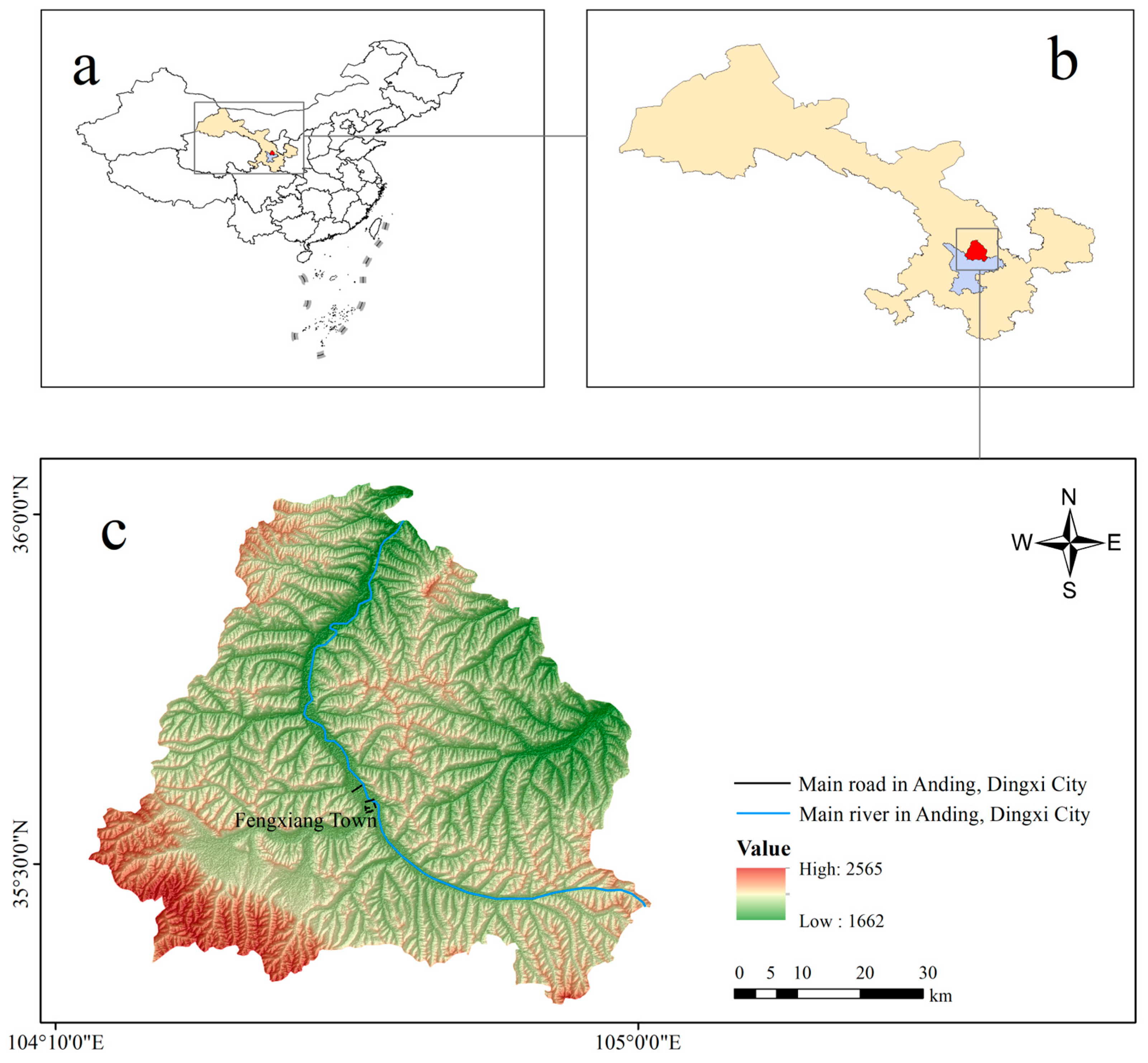
2.1. Overview of the Research Area
2.2. Soil, Meteorological, Crop Management, and Yield Data Inputs to the APSIM and ML Models
2.2.1. Soil Data
2.2.2. Meteorological Data
2.2.3. Crop Management Data
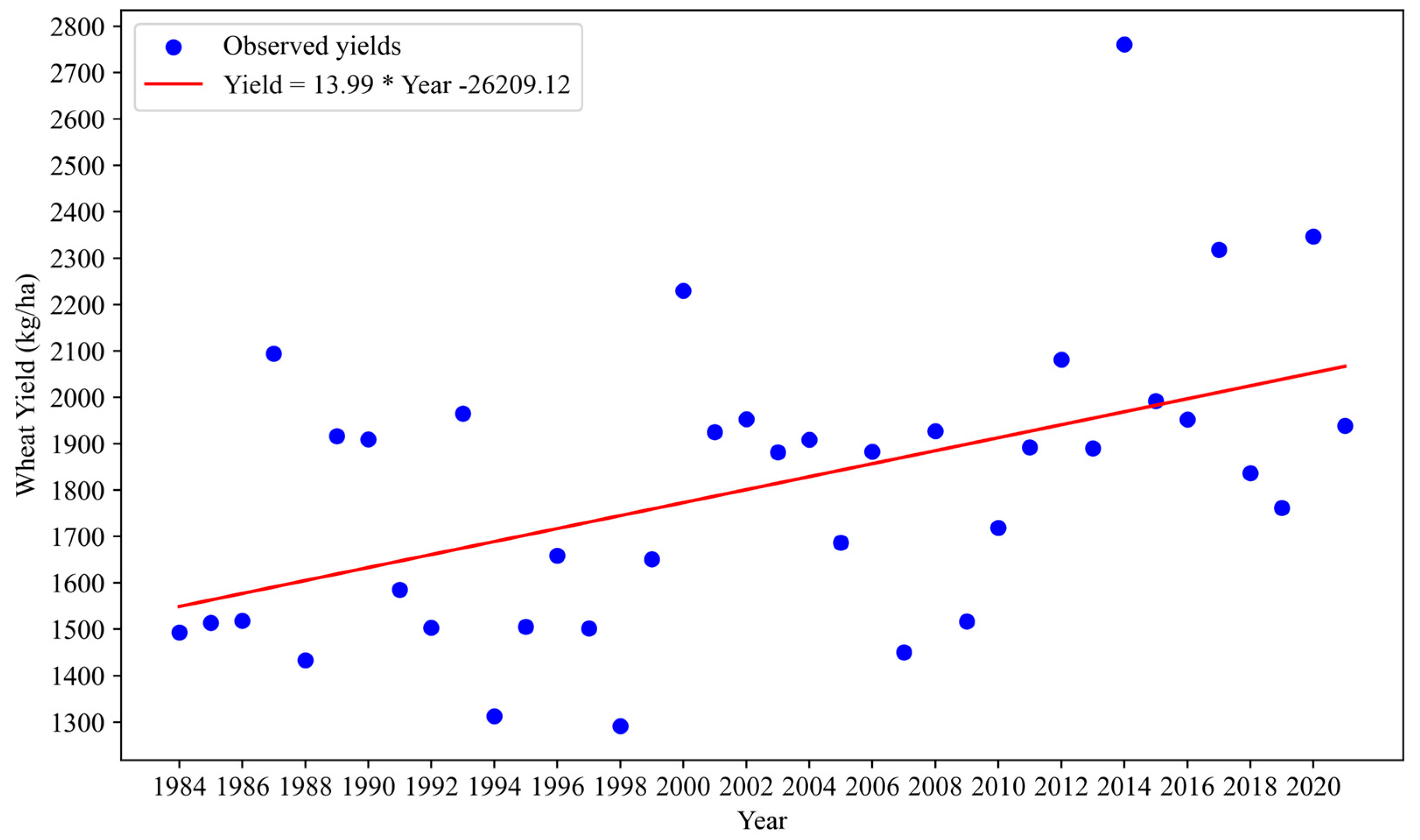
2.2.4. Crop Yield Data
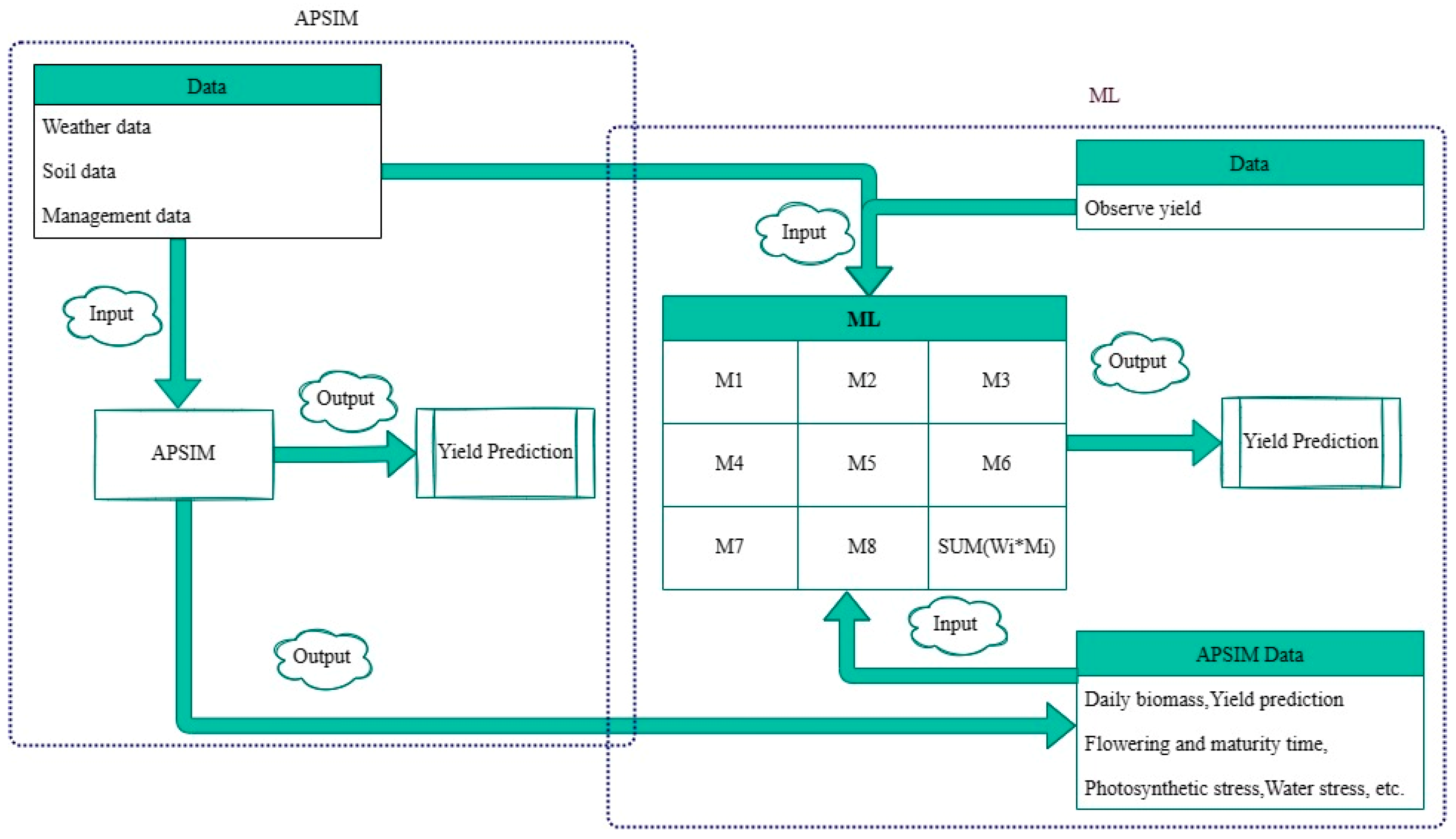
2.3. APSIM Model-Simulated Data Inputs to the ML Models
2.4. Data Preprocessing
2.4.1. Aggregation of All Data Sources and Unit Conversions
2.4.2. Imputation of Missing Values and Removal of Outliers
2.4.3. Construction of Features
2.4.4. Normalization of the Feature Data
2.4.5. Feature Selection
Expert Knowledge-Based Feature Selection
Permutation Feature Selection and Random Forests
2.5. Adjustment of Hyperparameters
2.6. Predictive Models
2.6.1. Agricultural Production Simulator (APSIM)
2.6.2. Eight Machine Learning Algorithms
2.6.3. Weighted Average Ensemble Model
2.6.4. Optimized Weighted Ensemble Model
- Set the model parameters (weights) to certain values.
- Compute the gradient of the loss function with respect to the parameters.
- Update the parameters in the direction opposite to the gradient to reduce the loss.
- Repeat the above steps until the loss reaches a satisfactory level or the maximum number of iterations is reached.
2.7. Evaluation Metrics
2.8. Experimental Environment Configuration
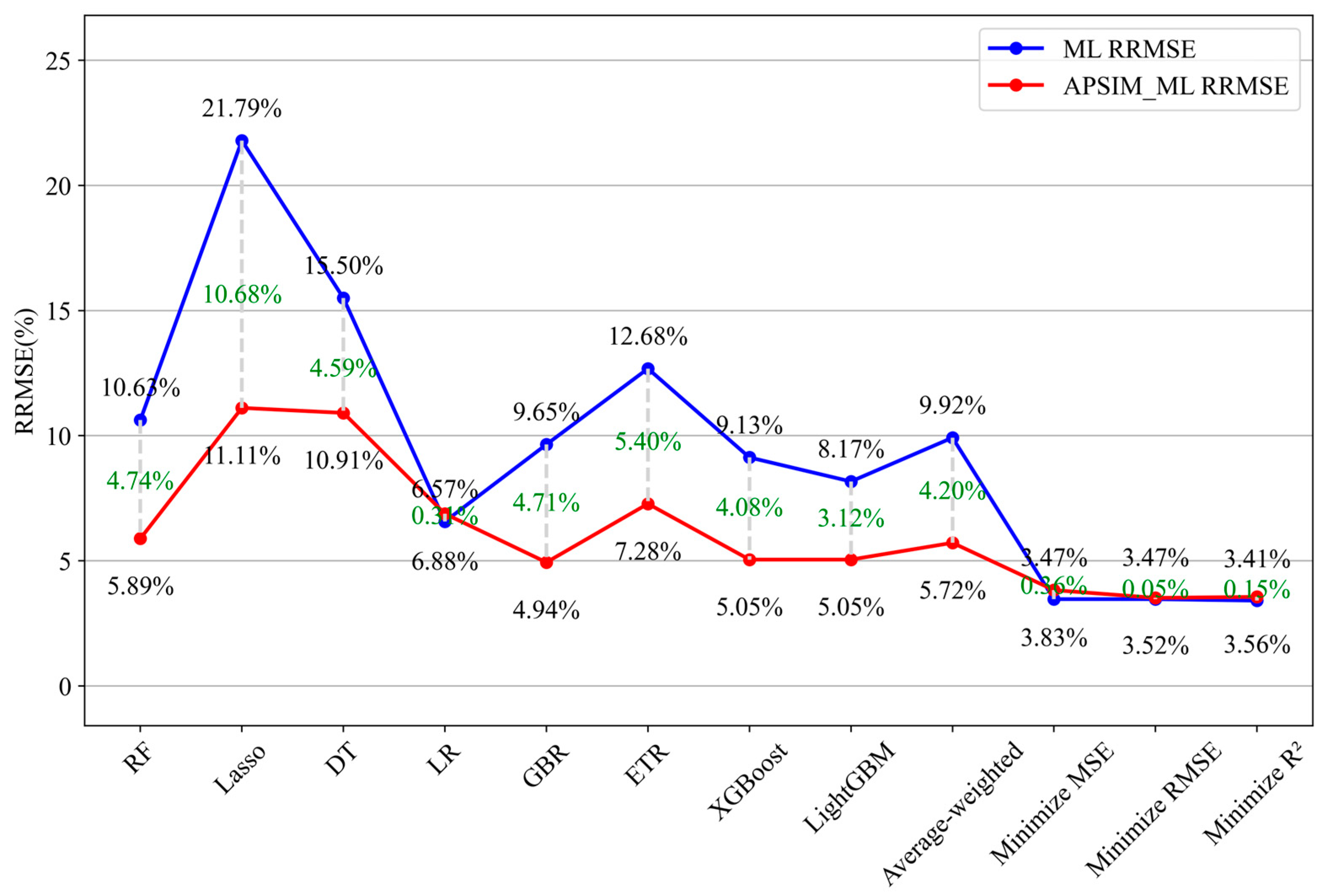
3. Results
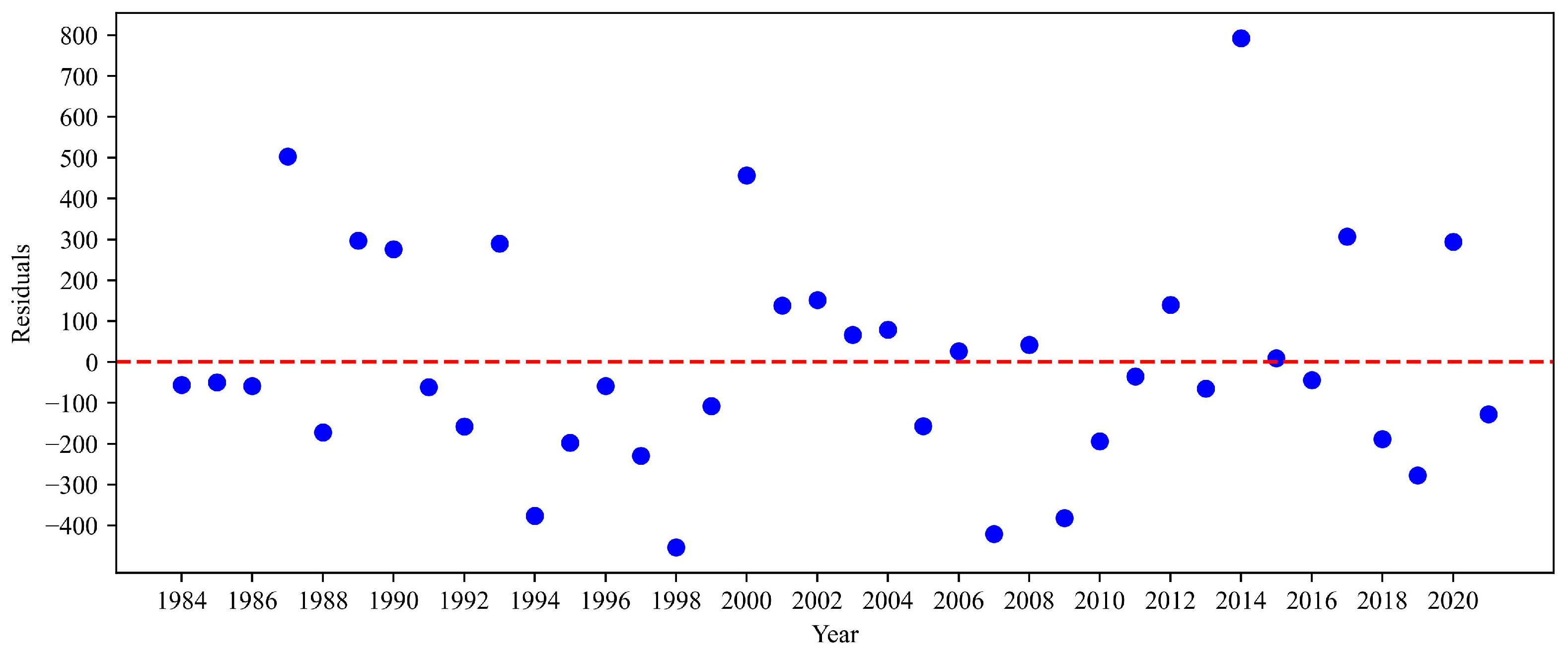
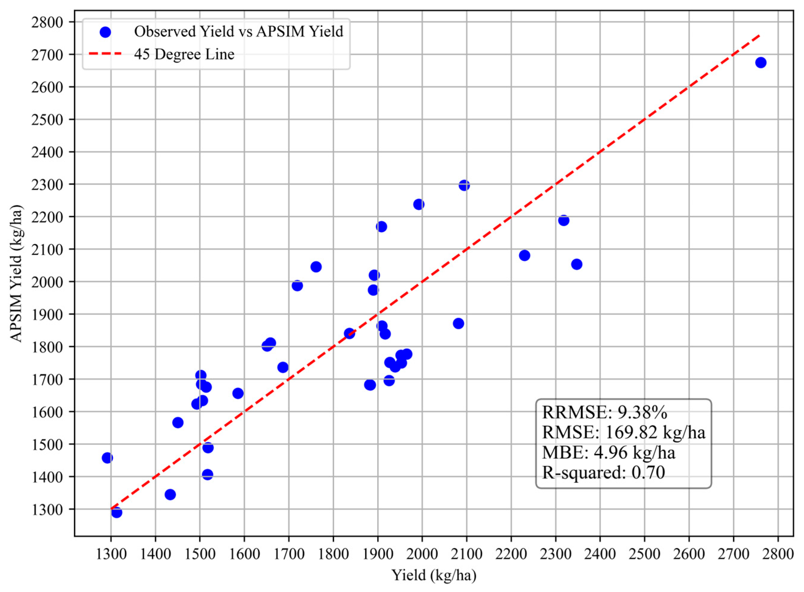
3.1. APSIM Model Performance Verification
3.2. Prediction of the Model Performance
3.3. Comparison and Analysis of Model Performance in Different Years
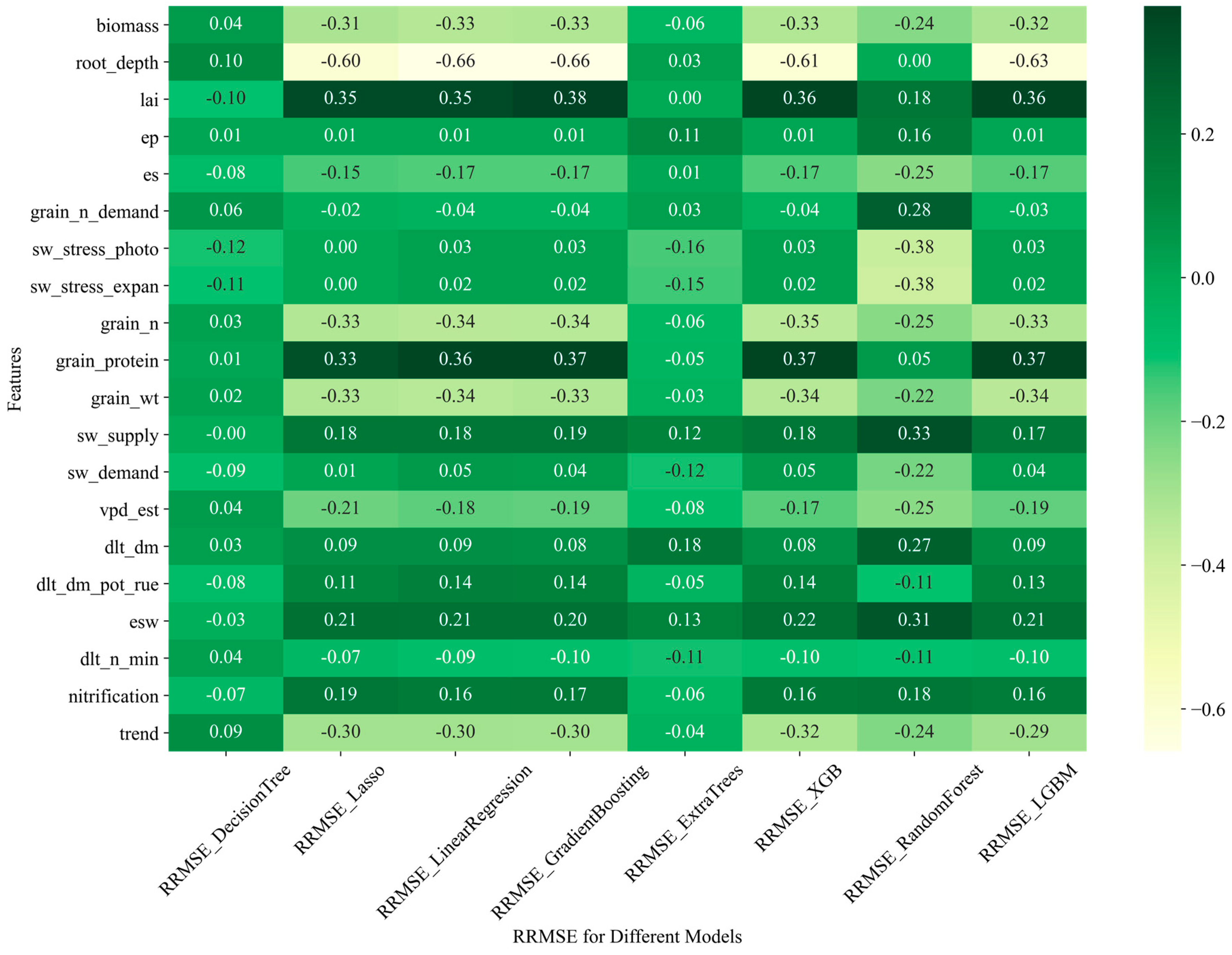
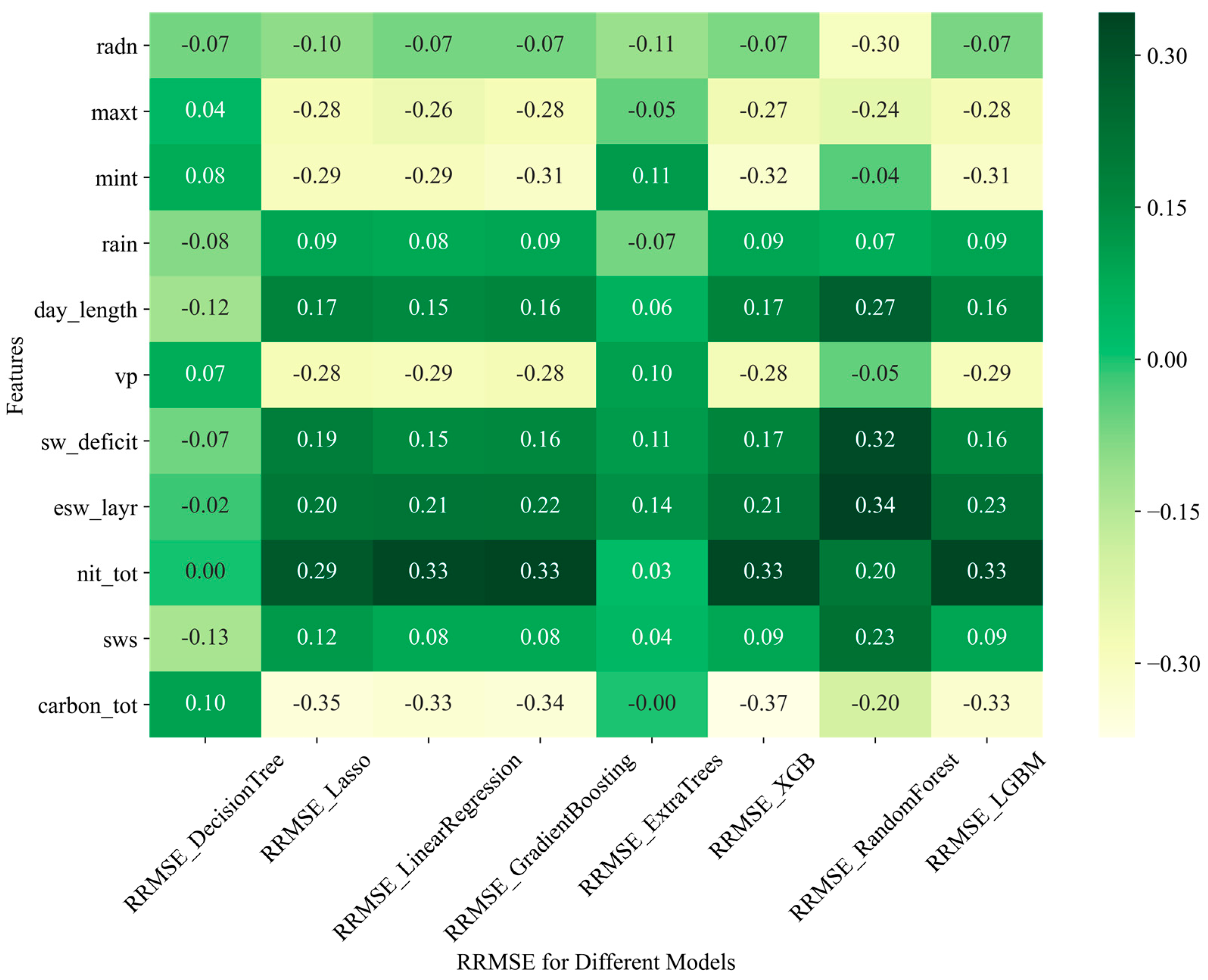
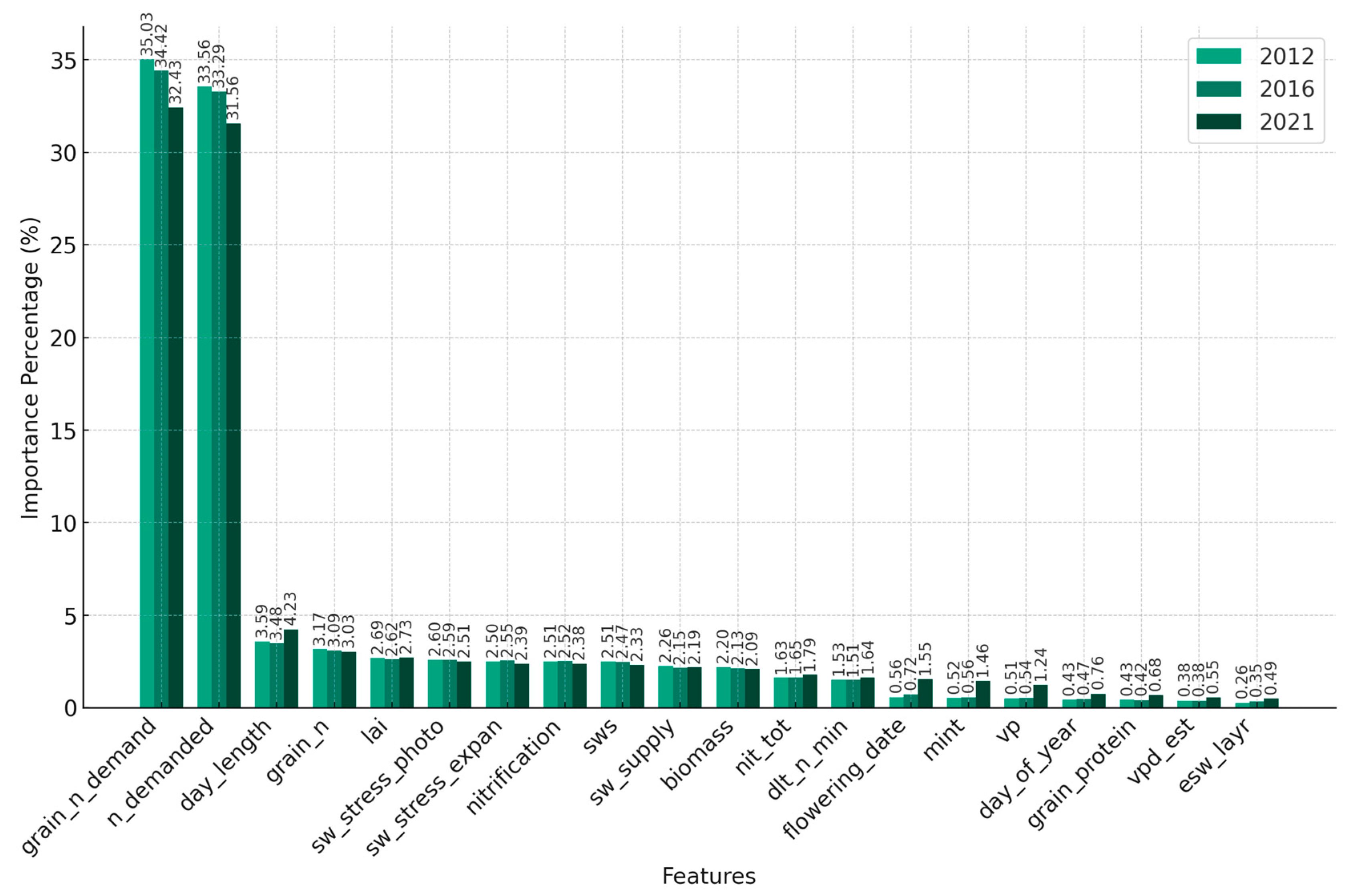
3.4. Relationship between APSIM-ML Model Performance and Input Features
3.4.1. Relationship of the Model Performance to Partial APSIM Output Variables and the Constructed Feature
3.4.2. Relationship of the Model Performance and Weather Features and the APSIM Output of Soil Variable
4. Discussion
5. Conclusions
Author Contributions
Funding
Data Availability Statement
Conflicts of Interest
References
- Asseng, S.; Zhu, Y.; Basso, B.; Wilson, T.; Cammarano, D. Simulation Modeling: Applications in Cropping Systems. In Encyclopedia of Agriculture and Food Systems; Van Alfen, N.K., Ed.; Academic Press: Cambridge, MA, USA, 2014; pp. 102–112. ISBN 9780080931395. [Google Scholar] [CrossRef]
- Ahmed, M.; Akram, M.N.; Asim, M.; Aslam, M.; Hassan, F.-U.; Higgins, S.; Stöckle, C.O.; Hoogenboom, G. Calibration and validation of APSIM-Wheat and CERES-Wheat for spring wheat under rainfed conditions: Models evaluation and application. Comput. Electron. Agric. 2016, 123, 384–401. [Google Scholar] [CrossRef]
- Shahhosseini, M.; Martinez-Feria, R.A.; Hu, G.; Archontoulis, S.V. Maize yield and nitrate loss prediction with machine learning algorithms. Environ. Res. Lett. 2019, 14, 124026. [Google Scholar] [CrossRef]
- Yu, D.; Zha, Y.; Shi, L.; Ye, H.; Zhang, Y. Improving sugarcane growth simulations by integrating multi-source observations into a crop model. Eur. J. Agron. 2022, 132, 126410. [Google Scholar] [CrossRef]
- Yang, W.; Guo, T.; Luo, J.; Zhang, R.; Zhao, J.; Warburton, M.L.; Xiao, Y.; Yan, J. Target-oriented prioritization: Targeted selection strategy by integrating organismal and molecular traits through predictive analytics in breeding. Genome Biol. 2022, 23, 80. [Google Scholar] [CrossRef] [PubMed]
- Wu, H.; Yue, Q.; Guo, P.; Xu, X.; Huang, X. Improving the AquaCrop model to achieve direct simulation of evapotranspiration under nitrogen stress and joint simulation-optimization of irrigation and fertilizer schedules. Agric. Water Manag. 2022, 266, 107599. [Google Scholar] [CrossRef]
- Husson, O.; Tano, B.F.; Saito, K. Designing low-input upland rice-based cropping systems with conservation agriculture for climate change adaptation: A six-year experiment in M’bé, Bouaké, Côte d’Ivoire. Field Crops Res. 2022, 277, 108418. [Google Scholar] [CrossRef]
- Basso, B.; Liu, L. Seasonal Crop Yield Forecast: Methods, Applications, and Accuracies. In Advances in Agronomy; Sparks, D.L., Ed.; Academic Press: Cambridge, MA, USA, 2019; Volume 154, pp. 201–255. [Google Scholar] [CrossRef]
- Feng, P.; Wang, B.; Liu, D.L.; Waters, C.; Xiao, D.; Shi, L.; Yu, Q. Dynamic Wheat Yield Forecasts Are Improved by a Hybrid Approach Using a Biophysical Model and Machine Learning Technique. Agric. For. Meteorol. 2020, 285–286, 107922. [Google Scholar] [CrossRef]
- Islam, S.S.; Arafat, A.C.; Hasan, A.K.; Khomphet, T.; Karim, R. Estimating the optimum dose of nitrogen fertilizer with climatic conditions on improving Boro rice (Oryza sativa) yield using DSSAT-Rice crop model. Res. Crops 2022, 23, 253–260. [Google Scholar] [CrossRef]
- Kipkulei, H.K.; Bellingrath-Kimura, S.D.; Lana, M.A.; Ghazaryan, G.; Baatz, R.; Boitt, M.K.; Chisanga, C.B.; Rotich, B.; Sieber, S. Assessment of Maize Yield Response to Agricultural Management Strategies Using the DSSAT–CERES-Maize Model in Trans Nzoia County in Kenya. Int. J. Plant Prod. 2022, 16, 557–577. [Google Scholar] [CrossRef]
- Zhao, P.; Zhou, Y.; Li, F.; Ling, X.; Deng, N.; Peng, S.; Man, J. The Adaptability of APSIM-Wheat Model in the Middle and Lower Reaches of the Yangtze River Plain of China: A Case Study of Winter Wheat in Hubei Province. Agronomy 2020, 10, 981. [Google Scholar] [CrossRef]
- Wang, Y.; Lv, J.; Wang, Y.; Sun, H.; Hannaford, J.; Su, Z.; Barker, L.J.; Qu, Y. Drought Risk Assessment of Spring Maize Based on APSIM Crop Model in Liaoning Province, China. Int. J. Disaster Risk Reduct. 2020, 45, 101483. [Google Scholar] [CrossRef]
- Morel, J.; Kumar, U.; Ahmed, M.; Bergkvist, G.; Lana, M.; Halling, M.; Parsons, D. Quantification of the Impact of Temperature, CO2, and Rainfall Changes on Swedish Annual Crops Production Using the APSIM Model. Front. Sustain. Food Syst. 2021, 5, 665025. [Google Scholar] [CrossRef]
- Vogeler, I.; Cichota, R.; Langer, S.; Thomas, S.; Ekanayake, D.; Werner, A. Simulating Water and Nitrogen Runoff with APSIM. Soil Tillage Res. 2023, 227, 105593. [Google Scholar] [CrossRef]
- Kumar, U.; Hansen, E.M.; Thomsen, I.K.; Vogeler, I. Performance of APSIM to Simulate the Dynamics of Winter Wheat Growth, Phenology, and Nitrogen Uptake from Early Growth Stages to Maturity in Northern Europe. Plants 2023, 12, 986. [Google Scholar] [CrossRef] [PubMed]
- Sharma, A.; Jain, A.; Gupta, P.; Chowdary, V. Machine Learning Applications for Precision Agriculture: A Comprehensive Review. IEEE Access 2021, 9, 4843–4873. [Google Scholar] [CrossRef]
- Liakos, K.G.; Busato, P.; Moshou, D.; Pearson, S.; Bochtis, D. Machine Learning in Agriculture: A Review. Sensors 2018, 18, 2674. [Google Scholar] [CrossRef] [PubMed]
- Zhang, C.; Park, D.S.; Yoon, S.; Zhang, S. Editorial: Machine learning and artificial intelligence for smart agriculture. Front. Plant Sci. 2022, 13, 1121468. [Google Scholar] [CrossRef]
- Cao, J.; Wang, H.; Li, J.; Tian, Q.; Niyogi, D. Improving the Forecasting of Winter Wheat Yields in Northern China with Machine Learning–Dynamical Hybrid Subseasonal-to-Seasonal Ensemble Prediction. Remote Sens. 2022, 14, 1707. [Google Scholar] [CrossRef]
- González Sánchez, A.; Frausto Solís, J.; Ojeda Bustamante, W. Predictive ability of machine learning methods for massive crop yield prediction. Span. J. Agric. Res. 2014, 12, 313. [Google Scholar] [CrossRef]
- Klompenburg, T.V.; Kassahun, A.; Catal, C. Crop yield prediction using machine learning: A systematic literature review. Comput. Electron. Agric. 2020, 177, 105709. [Google Scholar] [CrossRef]
- Morales, A.; Villalobos, F.J. Using machine learning for crop yield prediction in the past or the future. Front. Plant Sci. 2023, 14, 1128388. [Google Scholar] [CrossRef]
- Chlingaryan, A.; Sukkarieh, S.; Whelan, B. Machine learning approaches for crop yield prediction and nitrogen status estimation in precision agriculture: A review. Comput. Electron. Agric. 2018, 151, 61–69. [Google Scholar] [CrossRef]
- Yamparla, R.; Shaik, H.S.; Guntaka, N.S.P.; Marri, P.; Nallamothu, S. Crop yield prediction using Random Forest Algorithm. In Proceedings of the 2022 7th International Conference on Communication and Electronics Systems (ICCES), Coimbatore, India, 22–24 June 2022; pp. 1538–1543. [Google Scholar] [CrossRef]
- Burdett, H.; Wellen, C. Statistical and machine learning methods for crop yield prediction in the context of precision agriculture. Precis. Agric. 2022, 23, 1553–1574. [Google Scholar] [CrossRef]
- Paudel, D.; Boogaard, H.; de Wit, A.; van der Velde, M.; Claverie, M.; Nisini, L.; Janssen, S.; Osinga, S.; Athanasiadis, I.N. Machine learning for regional crop yield forecasting in Europe. Field Crops Res. 2022, 276, 108377. [Google Scholar] [CrossRef]
- Chergui, N. Durum wheat yield forecasting using machine learning. Artif. Intell. Agric. 2022, 6, 156–166. [Google Scholar] [CrossRef]
- Adisa, O.M.; Botai, J.O.; Adeola, A.M.; Hassen, A.; Botai, C.M.; Darkey, D.; Tesfamariam, E. Application of Artificial Neural Network for Predicting Maize Production in South Africa. Sustainability 2019, 11, 1145. [Google Scholar] [CrossRef]
- Nevavuori, P.; Narra, N.; Lipping, T. Crop yield prediction with deep convolutional neural networks. Comput. Electron. Agric. 2019, 163, 104859. [Google Scholar] [CrossRef]
- Ma, Y.; Zhang, Z.; Kang, Y.; Özdoğan, M. Corn yield prediction and uncertainty analysis based on remotely sensed variables using a Bayesian neural network approach. Remote Sens. Environ. 2021, 259, 112408. [Google Scholar] [CrossRef]
- Hara, P.; Piekutowska, M.; Niedbała, G. Selection of Independent Variables for Crop Yield Prediction Using Artificial Neural Network Models with Remote Sensing Data. Land 2021, 10, 609. [Google Scholar] [CrossRef]
- Aubakirova, G.; Ivel, V.; Gerassimova, Y.; Moldakhmetov, S.; Petrov, P. Application of Artificial Neural Network for Wheat Yield Forecasting. East.-Eur. J. Enterp. Technol. 2022, 117, 31. [Google Scholar] [CrossRef]
- Belouz, K.; Nourani, A.; Zereg, S.; Bencheikh, A. Prediction of Greenhouse Tomato Yield Using Artificial Neural Networks Combined with Sensitivity Analysis. Sci. Hortic. 2022, 293, 110666. [Google Scholar] [CrossRef]
- Srivastava, A.K.; Safaei, N.; Khaki, S.; Lopez, G.; Zeng, W.; Ewert, F.; Gaiser, T.; Rahimi, J. Winter Wheat Yield Prediction Using Convolutional Neural Networks from Environmental and Phenological Data. Sci. Rep. 2022, 12, 3215. [Google Scholar] [CrossRef] [PubMed]
- Khaki, S.; Wang, L.; Archontoulis, S.V. A CNN-RNN Framework for Crop Yield Prediction. Front. Plant Sci. 2020, 10, 1750. [Google Scholar] [CrossRef] [PubMed]
- Gavahi, K.; Abbaszadeh, P.; Moradkhani, H. DeepYield: A Combined Convolutional Neural Network with Long Short-Term Memory for Crop Yield Forecasting. Expert Syst. Appl. 2021, 184, 115511. [Google Scholar] [CrossRef]
- Zhang, N.; Zhou, X.; Kang, M.; Hu, B.-G.; Heuvelink, E.P.; Marcelis, L.F.M. Machine Learning Versus Crop Growth Models: An Ally, Not a Rival. AoB PLANTS 2023, 15, plac061. [Google Scholar] [CrossRef] [PubMed]
- Balakrishnan, N.; Muthukumarasamy, G. Crop Production-Ensemble Machine Learning Model for Prediction. Int. J. Comput. Sci. Softw. Eng. 2016, 5, 148. [Google Scholar]
- Zou, Y.; Kattel, G.R.; Miao, L. Enhancing Maize Yield Simulations in Regional China Using Machine Learning and Multi-Data Resources. Remote Sens. 2024, 16, 701. [Google Scholar] [CrossRef]
- Paudel, D.; Boogaard, H.; de Wit, A.; Janssen, S.; Osinga, S.; Pylianidis, C.; Athanasiadis, I.N. Machine Learning for Large-Scale Crop Yield Forecasting. Agric. Syst. 2021, 187, 103016. [Google Scholar] [CrossRef]
- Maharana, K.; Mondal, S.; Nemade, B. A Review: Data Pre-processing and Data Augmentation Techniques. Glob. Transit. Proc. 2022, 3, 91–99. [Google Scholar] [CrossRef]
- Jansen, B.J.; Aldous, K.K.; Salminen, J.; Almerekhi, H.; Jung, S.G. Data Preprocessing. In Understanding Audiences, Customers, and Users via Analytics: An Introduction to the Employment of Web, Social, and Other Types of Digital People Data; Springer Nature Switzerland: Cham, Switzerland, 2023; pp. 65–75. [Google Scholar] [CrossRef]
- Wang, T.C.; Casadebaig, P.; Chen, T.W. More than 1000 Genotypes Are Required to Derive Robust Relationships between Yield, Yield Stability and Physiological Parameters: A Computational Study on Wheat Crop. Theor. Appl. Genet. 2023, 136, 34. [Google Scholar] [CrossRef]
- Du, W. PyPOTS: A Python Toolbox for Data Mining on Partially-Observed Time Series. arXiv 2023, arXiv:2305.18811. [Google Scholar] [CrossRef]
- Maniraj, S.P.; Chaudhary, D.; Deep, V.H.; Singh, V.P. Data Aggregation and Terror Group Prediction Using Machine Learning Algorithms. Int. J. Recent Technol. Eng. 2019, 8, 1467–1469. [Google Scholar] [CrossRef]
- Jin, X.; Zhang, J.; Kong, J.; Su, T.; Bai, Y. A Reversible Automatic Selection Normalization (RASN) Deep Network for Predicting in the Smart Agriculture System. Agronomy 2022, 12, 591. [Google Scholar] [CrossRef]
- Strobl, C.; Boulesteix, A.; Zeileis, A.; Hothorn, T. Bias in Random Forest Variable Importance Measures: Illustrations, Sources and a Solution. BMC Bioinform. 2007, 8, 25. [Google Scholar] [CrossRef] [PubMed]
- Breiman, L. Random Forests. Mach. Learn. 2001, 45, 5–32. [Google Scholar] [CrossRef]
- Maciej, S.; Becker, F.G.; Cleary, M.; Team, R.M.; Holtermann, H.; The, D.; Agenda, N.; Science, P.; Sk, S.K.; Hinnebusch, R.; et al. Synteza i Aktywność Biologiczna Nowych Analogów Tiosemikarbazonowych Chelatorów Żelaza. Uniw. Śląski 2013, 7, 343–354. [Google Scholar]
- Altmann, A.; Toloși, L.; Sander, O.; Lengauer, T. Permutation Importance: A Corrected Feature Importance Measure. Bioinformatics 2010, 26, 1340–1347. [Google Scholar] [CrossRef]
- Molnar, C. Interpretable Machine Learning. 2020. Available online: https://Lulu.com (accessed on 2 October 2023).
- Garnett, R. Bayesian Optimization; Cambridge University Press: Cambridge, UK, 2023. [Google Scholar] [CrossRef]
- Snoek, J.; Larochelle, H.; Adams, R.P. Practical Bayesian Optimization of Machine Learning Algorithms. Adv. Neural Inf. Process. Syst. 2012, 25, 2951–2959. [Google Scholar]
- Wang, X.; Jin, Y.; Schmitt, S.; Olhofer, M. Recent Advances in Bayesian Optimization. ACM Comput. Surv. 2023, 55, 1–36. [Google Scholar] [CrossRef]
- Keating, B.A.; Carberry, P.S.; Hammer, G.L.; Probert, M.E.; Robertson, M.J.; Holzworth, D.; Huth, N.I.; Hargreaves, J.N.; Meinke, H.; Hochman, Z.; et al. An Overview of APSIM, a Model Designed for Farming Systems Simulation. Eur. J. Agron. 2003, 18, 267–288. [Google Scholar] [CrossRef]
- Holzworth, D.P.; Huth, N.I.; Voil, P.G.; Zurcher, E.J.; Herrmann, N.I.; McLean, G.; Chenu, K.; Oosterom, E.J.; Snow, V.O.; Murphy, C.; et al. APSIM—Evolution Towards a New Generation of Agricultural Systems Simulation. Environ. Model. Softw. 2014, 62, 327–350. [Google Scholar] [CrossRef]
- Brown, H.; Huth, N.; Holzworth, D. Crop Model Improvement in APSIM: Using Wheat as a Case Study. Eur. J. Agron. 2018, 100, 141–150. [Google Scholar] [CrossRef]
- Zhao, G.; Bryan, B.A.; Song, X. Sensitivity and Uncertainty Analysis of the APSIM-Wheat Model: Interactions between Cultivar, Environmental, and Management Parameters. Ecol. Model. 2014, 279, 1–11. [Google Scholar] [CrossRef]
- Zhang, Y.; Walker, J.P.; Pauwels, V.R.N.; Sadeh, Y. Assimilation of Wheat and Soil States into the APSIM-Wheat Crop Model: A Case Study. Remote Sens. 2022, 14, 65. [Google Scholar] [CrossRef]
- Zhang, Y.; Feng, L.; Wang, E.; Wang, J.; Li, B. Evaluation of the APSIM-Wheat Model in Terms of Different Cultivars, Management Regimes and Environmental Conditions. Can. J. Plant Sci. 2012, 92, 937–949. [Google Scholar] [CrossRef]
- James, G.; Witten, D.; Hastie, T.; Tibshirani, R.; Taylor, J. Statistical Learning. In An Introduction to Statistical Learning; Springer Texts in Statistics; Springer: Cham, Switzerland, 2023. [Google Scholar] [CrossRef]
- Tibshirani, R. Regression Shrinkage and Selection via the Lasso. J. R. Stat. Soc. Ser. B 1996, 58, 267–288. [Google Scholar] [CrossRef]
- Ranstam, J.; Cook, J.A. LASSO Regression. Br. J. Surg. 2018, 105, 1348. [Google Scholar] [CrossRef]
- Bansal, M.; Goyal, A.; Choudhary, A. A Comparative Analysis of K-Nearest Neighbor, Genetic, Support Vector Machine, Decision Tree, and Long Short Term Memory Algorithms in Machine Learning. Decis. Anal. J. 2022, 3, 100071. [Google Scholar] [CrossRef]
- Suresh, N.; Ramesh, N.V.K.; Inthiyaz, S.; Priya, P.P.; Nagasowmika, K.; Kumar, K.V.N.H.; Shaik, M.; Reddy, B.N.K. Crop Yield Prediction Using Random Forest Algorithm. In Proceedings of the 2021 7th International Conference on Advanced Computing and Communication Systems (ICACCS), Coimbatore, India, 19–20 March 2021; pp. 279–282. [Google Scholar] [CrossRef]
- Cutler, D.R.; Edwards, T.C., Jr.; Beard, K.H.; Cutler, A.; Hess, K.T.; Gibson, J.; Lawler, J.J. Random Forests for Classification in Ecology. Ecology 2007, 88, 2783–2792. [Google Scholar] [CrossRef]
- Chen, T.; Guestrin, C. XGBoost: A Scalable Tree Boosting System. In Proceedings of the 22nd ACM SIGKDD International Conference on Knowledge Discovery and Data Mining, San Francisco, CA, USA, 13–17 August 2016; pp. 785–794. [Google Scholar] [CrossRef]
- Ke, G.; Meng, Q.; Finley, T.; Wang, T.; Chen, W.; Ma, W.; Ye, Q.; Liu, T. LightGBM: A Highly Efficient Gradient Boosting Decision Tree. Neural Information Processing Systems. 2017. Available online: https://api.semanticscholar.org/CorpusID:3815895 (accessed on 2 October 2023).
- Friedman, J.H. Greedy Function Approximation: A Gradient Boosting Machine. Ann. Statist. 2001, 29, 1189–1232. Available online: http://www.jstor.org/stable/2699986 (accessed on 2 October 2023). [CrossRef]
- Friedman, J.H. Stochastic Gradient Boosting. Comput. Stat. Data Anal. 2002, 38, 367–378. [Google Scholar] [CrossRef]
- Geurts, P.; Ernst, D.; Wehenkel, L. Extremely Randomized Trees. Mach. Learn. 2006, 63, 3–42. [Google Scholar] [CrossRef]
- Shang, K.; Yao, Y.; Li, Y.; Yang, J.; Jia, K.; Zhang, X.; Chen, X.; Bei, X.; Guo, X. Fusion of Five Satellite-Derived Products Using Extremely Randomized Trees to Estimate Terrestrial Latent Heat Flux Over Europe. Remote Sens. 2020, 12, 687. [Google Scholar] [CrossRef]
- Mienye, I.D.; Sun, Y. A Survey of Ensemble Learning: Concepts, Algorithms, Applications, and Prospects. IEEE Access 2022, 10, 99129–99149. [Google Scholar] [CrossRef]
- Shahhosseini, M.; Hu, G.; Pham, H. Optimizing Ensemble Weights and Hyperparameters of Machine Learning Models for Regression Problems. Mach. Learn. Appl. 2022, 7, 100251. [Google Scholar] [CrossRef]
- Sammut, C.; Webb, G. Encyclopedia of Machine Learning and Data Mining; Springer Publishing Company: Berlin/Heidelberg, Germany, 2017. [Google Scholar] [CrossRef]
- Zhou, Z.H. Ensemble Learning. In Machine Learning; Springer: Singapore, 2021; pp. 149–171. [Google Scholar] [CrossRef]
- Shahhosseini, M.; Hu, G.; Pham, H. Optimizing Ensemble Weights for Machine Learning Models: A Case Study for Housing Price Prediction. In Smart Service Systems, Operations Management, and Analytics. INFORMS-CSS 2019; Springer Proceedings in Business and Economics; Springer: Cham, Switzerland, 2020; pp. 123–136. [Google Scholar] [CrossRef]
- Zheng, A.; Shelby, N.; Volckhausen, E. Evaluating Machine Learning Models. In Machine Learning in the AWS Cloud; Wiley: Hoboken, NJ, USA, 2019. [Google Scholar] [CrossRef]
- Mathieu, J.A.; Aires, F. Assessment of Agro-Climatic Indices for Enhancing Crop Yield Forecasting. Agric. For. Meteorol. 2018, 253–254, 15–30. [Google Scholar] [CrossRef]
- Franz, T.E.; Pokal, S.; Gibson, J.P.; Zhou, Y.; Gholizadeh, H.; Tenorio, F.A.; Rudnick, D.; Heeren, D.; McCabe, M.; Ziliani, M.; et al. The Role of Topography, Soil, and Remotely Sensed Vegetation Condition in Predicting Crop Yield. Field Crops Res. 2020, 252, 107788. [Google Scholar] [CrossRef]
- Dai, X.; Huo, Z.; Wang, H. Simulation for Response of Crop Yield to Soil Moisture and Salinity with Artificial Neural Network. Field Crops Res. 2011, 121, 441–449. [Google Scholar] [CrossRef]
- Guo, L.; Yang, Y.; Zhao, Y.; Li, Y.; Sui, Y.; Tang, C.; Jin, J.; Liu, X. Reducing Topsoil Depth Decreases the Yield and Nutrient Uptake of Maize and Soybean Grown in a Glacial Till. Land Degrad. Dev. 2021, 32, 2849–2860. [Google Scholar] [CrossRef]
- Jiang, H.; Hu, H.; Li, B.; Zhang, Z.; Wang, S.; Lin, T. Understanding the Non-stationary Relationships Between Corn Yields and Meteorology via a Spatiotemporally Varying Coefficient Model. Agric. For. Meteorol. 2021, 301–302, 108340. [Google Scholar] [CrossRef]


| Study | Model | Key Findings | Reference |
|---|---|---|---|
| Islam et al. | DSSAT (rice) | The BRRI dhan 29 variety showed the best performance under a nitrogen fertilizer treatment of 150 kg/ha, yielding 6000 kg/ha. | [10] |
| Kipkulei et al. | DSSAT-CERES (maize) | In Trans Nzoia County, Kenya, the KH600-23A maize variety outperformed H614 by 7.1% under the optimal nitrogen application strategy of 100 kg/ha in mid-February. | [11] |
| Zhao et al. | APSIM-Wheat | A strong positive correlation (R2: 0.90–0.97) was found between the predicted and observed wheat growth durations in the middle and lower reaches of the Yangtze River Plain, indicating the high predictive accuracy of the model. | [12] |
| Wang et al. | APSIM (maize) | The APSIM model assessment of drought risk in Liaoning showed that spring maize in the Chaoyang and Fuxin districts faces the highest drought risk. | [13] |
| Morel et al. | APSIM (annual crops) | In Sweden’s high latitude areas, a temperature increase of 1 °C maximizes barley and oats yields, while a 2–3 °C increase optimizes silage maize production. | [14] |
| Vogeler et al. | APSIM (runoff) | The study highlighted the significant impact of rainfall intensity and surface conductivity on water and nitrogen runoff loss in poorly drained clay soils. | [15] |
| Kumar et al. | APSIM (wheat phenology) | High accuracy in simulating winter wheat phenological stages in Nordic regions was achieved with an r2 of 0.97 and RMSE of 3.98–4.15 on the BBCH scale. | [16] |
| Study | ML Model | Key Findings | Reference |
|---|---|---|---|
| Yamparla et al. | Various (Gradient Boosting, Linear Regression, etc.) | Random forest achieved 95% accuracy in predicting crop yields in India, standing out among various machine learning techniques based on extensive historical and environmental data. | [25] |
| Burdett and Wellen | Random Forest, Decision Tree | In southwestern Ontario, Random Forest and Decision Tree models showed superior yield prediction for corn and soybean, analyzing soil attributes across 17 fields. | [26] |
| Paudel et al. | Machine Learning-based Method | A machine learning method for regional crop yield prediction in Europe was introduced, outperforming traditional models with lower errors, especially effectively close to the harvesting time. | [27] |
| Chergui | Deep Neural Network, Random Forest | Enhanced wheat yield predictions in two Algerian provinces through data augmentation, with a Deep Neural Network leading in one (RMSE of 4 kg/ha) and Random Forest in another (RMSE of 5 kg/ha). | [28] |
| Recently, Neural Network-based crop yield prediction models have also demonstrated exceptional accuracy [29,30,31,32,33,34]. | |||
| Srivastava et al. | Convolutional Neural Network (CNN) | A CNN model for winter wheat yield prediction in Germany reduced the RMSE and MAE significantly, showing high accuracy over other machine learning models in a 20-year dataset. | [35] |
| Khaki et al. | Residual Neural Network (CNN and RNN) | A Residual Neural Network was employed for corn and soybean yield prediction in the U.S., revealing critical insights into temporal variations through environmental and operational data. | [36] |
| Gavahi et al. | Deep Yield (ConvLSTM with 3DCNN) | The Deep Yield model, using ConvLSTM and 3DCNN and trained on historical soybean data and MODIS imagery, outshone traditional models in predictive accuracy across the U.S. | [37] |
| Parameter | Soil Depth (mm) | ||||||||
|---|---|---|---|---|---|---|---|---|---|
| 0–50 | 50–100 | 100–300 | 300–500 | 500–800 | 800–1100 | 1100–1400 | 1400–1700 | 1700–2000 | |
| Bulk density (g/cm3) | 1.29 | 1.23 | 1.33 | 1.20 | 1.14 | 1.14 | 1.25 | 1.12 | 1.11 |
| pH (1:5 water) | 8.320 | 8.370 | 8.330 | 8.300 | 8.320 | 8.370 | 8.420 | 8.430 | 8.400 |
| Air-dried moisture (mm/mm) | 0.01 | 0.01 | 0.05 | 0.07 | 0.09 | 0.10 | 0.11 | 0.12 | 0.13 |
| Wilting coefficient (mm/mm) | 0.09 | 0.09 | 0.09 | 0.09 | 0.09 | 0.11 | 0.11 | 0.12 | 0.13 |
| Field capacity (mm/mm) | 0.27 | 0.27 | 0.27 | 0.27 | 0.26 | 0.27 | 0.26 | 0.26 | 0.26 |
| Saturated moisture (mm/mm) | 0.46 | 0.49 | 0.45 | 0.50 | 0.52 | 0.52 | 0.48 | 0.53 | 0.53 |
| Lower available moisture (mm/mm) | 0.09 | 0.09 | 0.09 | 0.09 | 0.10 | 0.12 | 0.13 | 0.18 | 0.22 |
| Soil water conductivity (mm/h) | 0.60 | 0.60 | 0.60 | 0.60 | 0.60 | 0.60 | 0.60 | 0.60 | 0.60 |
| Acronym | Description |
|---|---|
| day_of_year | Day of year (day) |
| Yield | Crop yield (kg/ha) |
| Biomass | Crop biomass (kg/ha) |
| root_depth | Depth of roots (mm) |
| flowering_date | Day number of flowering (doy) |
| maturity_date | Day number of maturity (doy) |
| Lai | Leaf area index (m2/m2) |
| Ep | Plant water uptake (mm) |
| Es | Evaporation from soil (mm) |
| N_demanded | N demand of plant (g/m2) |
| grain_n_demand | N demand of grain (g/m2) |
| grain_wt | Weight of grain (g/m2) |
| Grain1GrainTotalN | GrainTotal Grain1 nitrogen (g/m2) |
| sw_stress_photo | Soil water stress for photosynthesis (0–1) |
| sw_stress_expan | Soil water stress for leaf expansion (0–1) |
| water_table | Water table depth (mm) |
| Runoff | Runoff (mm) |
| dlt_n_min_tot | Humic N mineralization (kg/ha) |
| Nitrification | Nitrogen moved by nitrification (kg/ha) |
| dlt_n_min | Het N mineralization (kg/ha) |
| Sws | Soil water (mm/mm) |
| sw_supply | Soil water supply (mm) |
| sw_demand | Demand for soil water (mm) |
| sw_deficit | Soil water deficit (mm) |
| vpd_est | Estimated vapor pressure deficit (kPa) |
| esw_layr | Extractable soil water (mm) |
| dlt_dm | Actual above-ground dry matter production (g/m2) |
| dlt_dm_pot_rue | Potential above-ground dry matter production via photosynthesis (g/m2) |
| day_of_year | grain_n_demand | grain_size | radn | sws | trend | grain_size | GrowthN | leaf_no | n_demand_head |
| yield | sw_stress_photo | grain_wt | maxt | dul | dnit | grain_protein | GrowthP | LeafDetachingN | n_supply_soil |
| biomass | sw_stress_expan | Grain1GrainTotalN | mint | sat | cover_green | Grain1DetachingN | GrowthWt | LeafDetachingP | n_uptake |
| root_depth | water_table | sw_supply | rain | swcon | dlt_lai | Grain1DetachingP | HeadGreenWt | LeafDetachingWt | p_conc_stover |
| flowering_date | runoff | sw_demand | day_length | nit_tot | dlt_n_fixed | Grain1DetachingWt | HeadGrowthN | LeafTotalP | p_demand |
| maturity_date | dlt_n_min_tot | sw_deficit | vp | ll15_dep | dlt_Pai | green_biomass | HeadGrowthP | LeafTotalpconc | p_uptake |
| lai | nitrification | vpd_est | air_dry | ll_dep | dm_plant_min | green_biomass_n | HeadGrowthWt | n_conc_crit | Pai |
| ep | dlt_n_min | esw_layr | bd | LL15 | effective_rue | green_biomass_p | lai_sum | n_conc_crit_grain | SenescedN |
| es | grain_n | dlt_dm | carbon_tot | PH | grain_p | green_biomass_wt | leaf_area | n_conc_grain | sowing_date |
| n_demanded | grain_protein | dlt_dm_pot_rue | esw | fertiliser | grain_wt | GreenWt | TTAfteremergence | n_demand_grain | Stage |
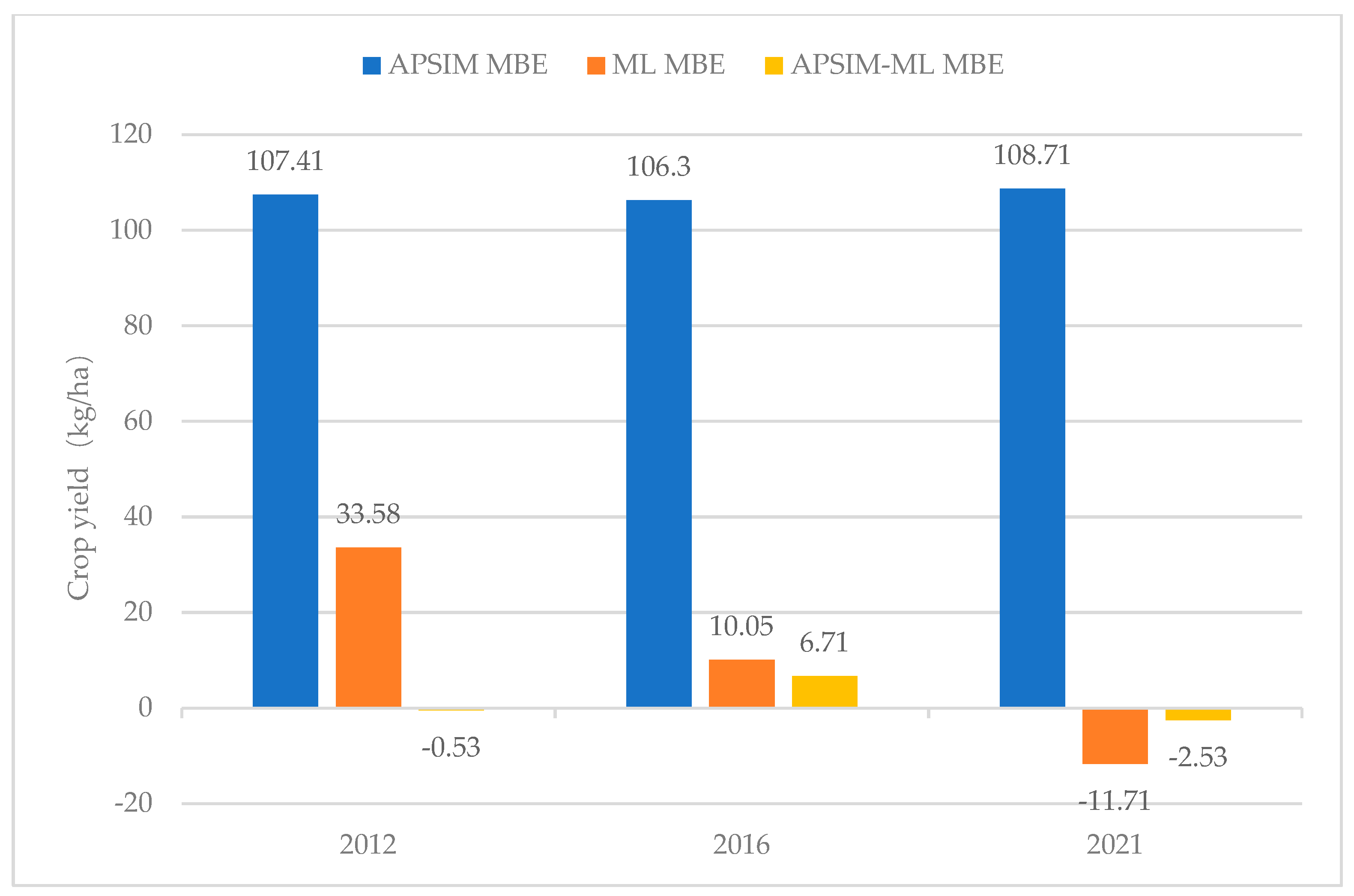
| Year | RMSE (kg/ha) | RRMSE (%) | MBE (kg/ha) | R2 |
|---|---|---|---|---|
| 2012 | 134.11 | 10.69 | 107.41 | 0.9573 |
| 2016 | 133.63 | 9.93 | 106.30 | 0.9616 |
| 2021 | 135.67 | 11.71 | 108.71 | 0.9613 |
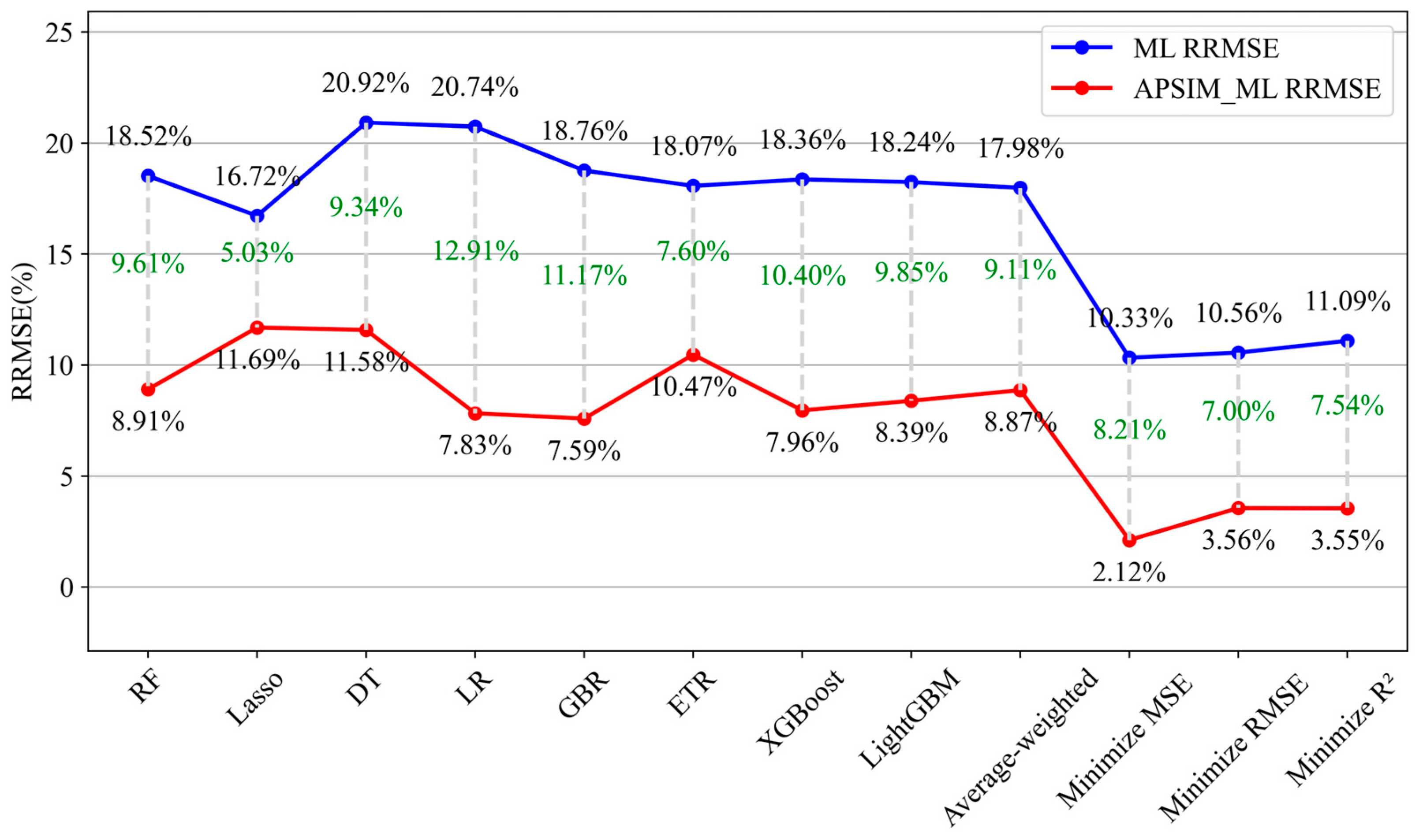
| ML Model | RMSE (kg/ha) | RRMSE (%) | MBE (kg/ha) | R2 | APSIM-ML Model | RMSE (kg/ha) | RRMSE (%) | MBE (kg/ha) | R2 | Increase in RRMSE (%) |
|---|---|---|---|---|---|---|---|---|---|---|
| Random Forest | 231.68 | 18.52 | 199.71 | 0.8744 | APSIM-Random Forest | 111.62 | 8.91 | 94.31 | 0.9737 | −9.61 |
| Lasso Regression | 208.63 | 16.72 | 107.07 | 0.8952 | APSIM-Lasso Regression | 146.09 | 11.69 | 116.65 | 0.9462 | −5.03 |
| Decision Tree | 260.54 | 20.92 | 208.15 | 0.8376 | APSIM-Decision Tree | 144.71 | 11.58 | 113.63 | 0.9463 | −9.34 |
| Linear Regression | 259.41 | 20.74 | 242.1 | 0.8375 | APSIM-Linear Regression | 97.92 | 7.83 | 79.83 | 0.9742 | −12.91 |
| Gradient Boosting | 234.04 | 18.76 | 200.57 | 0.8702 | APSIM-Gradient Boosting | 94.62 | 7.59 | 74.22 | 0.9752 | −11.17 |
| Extra Trees | 228.07 | 18.07 | 186.7 | 0.8767 | APSIM-Extra Trees | 130.89 | 10.47 | 110.43 | 0.9608 | −7.60 |
| XGBoost | 229.76 | 18.36 | 196.47 | 0.8743 | APSIM-XGBoost | 99.80 | 7.96 | 78.26 | 0.9760 | −10.4 |
| LightGBM | 229.18 | 18.24 | 191.82 | 0.8751 | APSIM-LightGBM | 105.05 | 8.39 | 78.68 | 0.9743 | −9.85 |
| Weighted Average Ensemble | 225.75 | 17.98 | 191.83 | 0.8785 | Weighted Average Ensemble | 110.95 | 8.87 | 93.19 | 0.9713 | −9.11 |
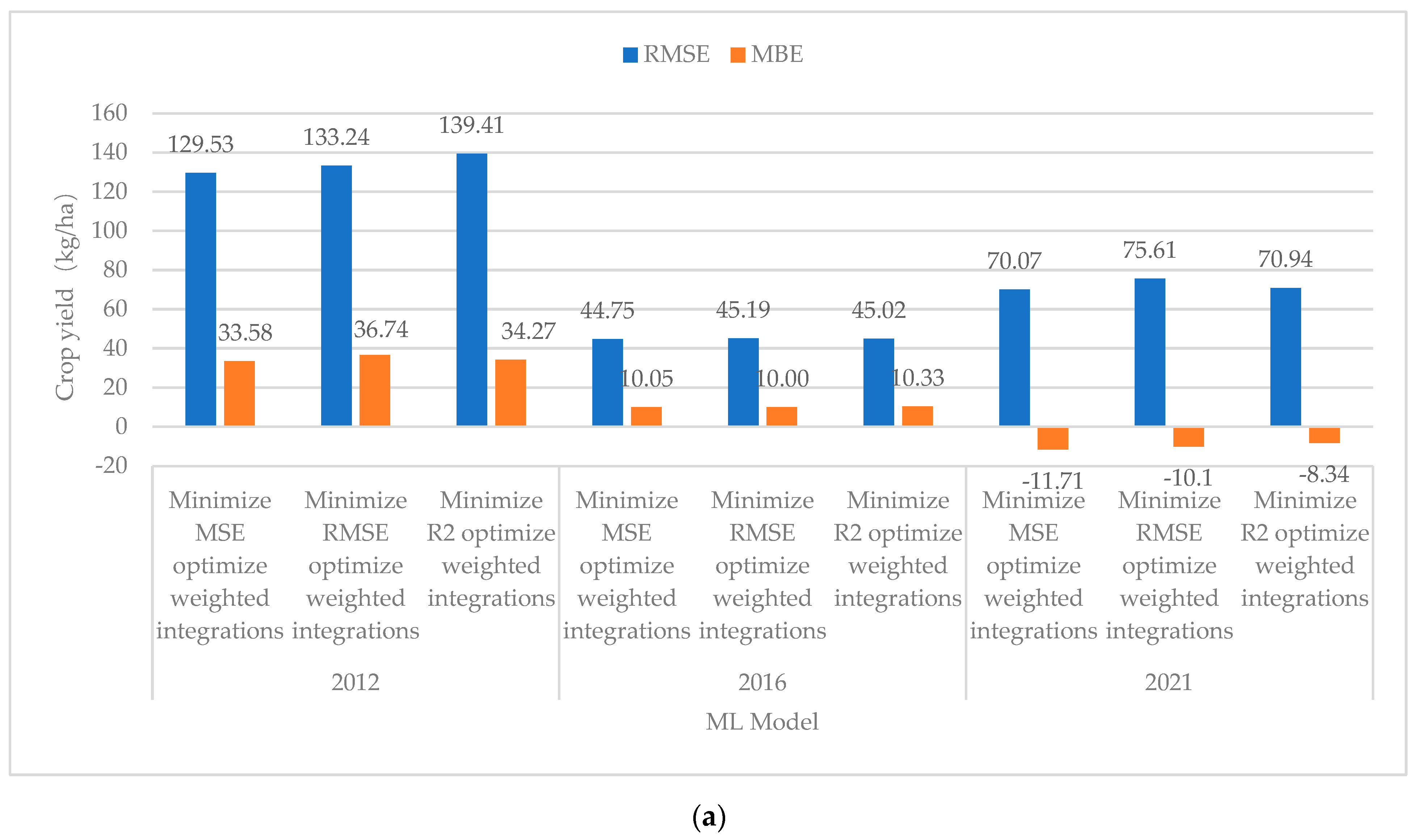
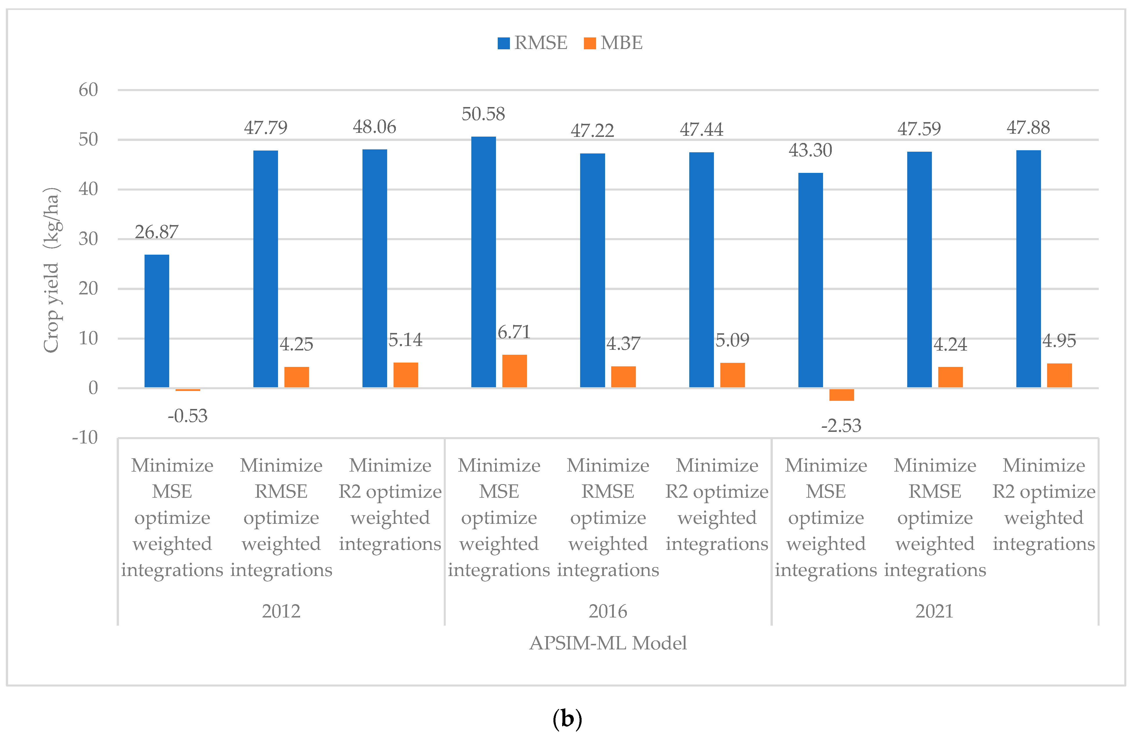
| Minimized MSE Optimized Weighted Integrations | 129.53 | 10.33 | 33.58 | 0.9608 | Minimized MSE Optimized Weighted Integrations | 26.78 | 2.12 | −0.53 | 0.9978 | −8.21 |
| Minimized RMSE Optimized Weighted Integrations | 133.24 | 10.56 | 36.74 | 0.9577 | Minimized RMSE Optimized Weighted Integrations | 47.66 | 3.56 | 4.25 | 0.9948 | −7.00 |
| Minimized R2 Optimized Weighted Integrations | 139.41 | 11.09 | 34.27 | 0.9541 | Minimized R2 Optimized Weighted Integrations | 47.93 | 3.55 | 5.14 | 0.9947 | −7.54 |
| ML Model | RMSE (kg/ha) | RRMSE (%) | MBE (kg/ha) | R2 | APSIM-ML Model | RMSE (kg/ha) | RRMSE (%) | MBE (kg/ha) | R2 | Increase in RRMSE (%) |
|---|---|---|---|---|---|---|---|---|---|---|
| Random Forest | 142.76 | 10.63 | 115.76 | 0.9347 | APSIM-Random Forest | 79.15 | 5.89 | 58.93 | 0.9827 | −4.74 |
| Lasso Regression | 296.16 | 21.79 | 154.49 | 0.8045 | APSIM-Lasso Regression | 150.68 | 11.11 | 120.35 | 0.952 | −10.68 |
| Decision Tree | 217.07 | 15.5 | 90.13 | 0.9013 | APSIM-Decision Tree | 147.05 | 10.91 | −5.67 | 0.9549 | −4.59 |
| Linear Regression | 83.93 | 6.57 | 54.02 | 0.9821 | APSIM-Linear Regression | 92.07 | 6.88 | 67.51 | 0.9733 | 0.31 |
| Gradient Boosting | 123.88 | 9.65 | 90.49 | 0.9656 | APSIM-Gradient Boosting | 66.69 | 4.94 | 24.95 | 0.9806 | −4.71 |
| Extra Trees | 173.15 | 12.68 | 144.89 | 0.9405 | APSIM-Extra Trees | 98.92 | 7.28 | 73.77 | 0.96 | −5.4 |
| XGBoost | 128.8 | 9.13 | 91.04 | 0.9657 | APSIM-XGBoost | 67.36 | 5.05 | 25.87 | 0.9805 | −4.08 |
| LightGBM | 108.21 | 8.17 | 96.9 | 0.9744 | APSIM-LightGBM | 67.63 | 5.05 | 21.01 | 0.9804 | −3.12 |
| Weighted Average Ensemble | 118.61 | 9.92 | −39.3 | 0.9725 | Weighted Average Ensemble | 77.09 | 5.72 | 57.88 | 0.9774 | −4.2 |
| Minimized MSE Optimized Weighted Integrations | 44.75 | 3.47 | 10.05 | 0.9952 | Minimized MSE Optimized Weighted Integrations | 50.58 | 3.83 | 6.71 | 0.9916 | 0.36 |
| Minimized RMSE Optimized Weighted Integrations | 45.19 | 3.47 | 10.00 | 0.9952 | Minimized RMSE Optimized Weighted Integrations | 47.22 | 3.52 | 4.37 | 0.9925 | 0.05 |
| Minimized R2 Optimized Weighted Integrations | 45.02 | 3.41 | 10.33 | 0.9952 | Minimized R2 Optimized Weighted Integrations | 47.44 | 3.56 | 5.09 | 0.9924 | 0.15 |
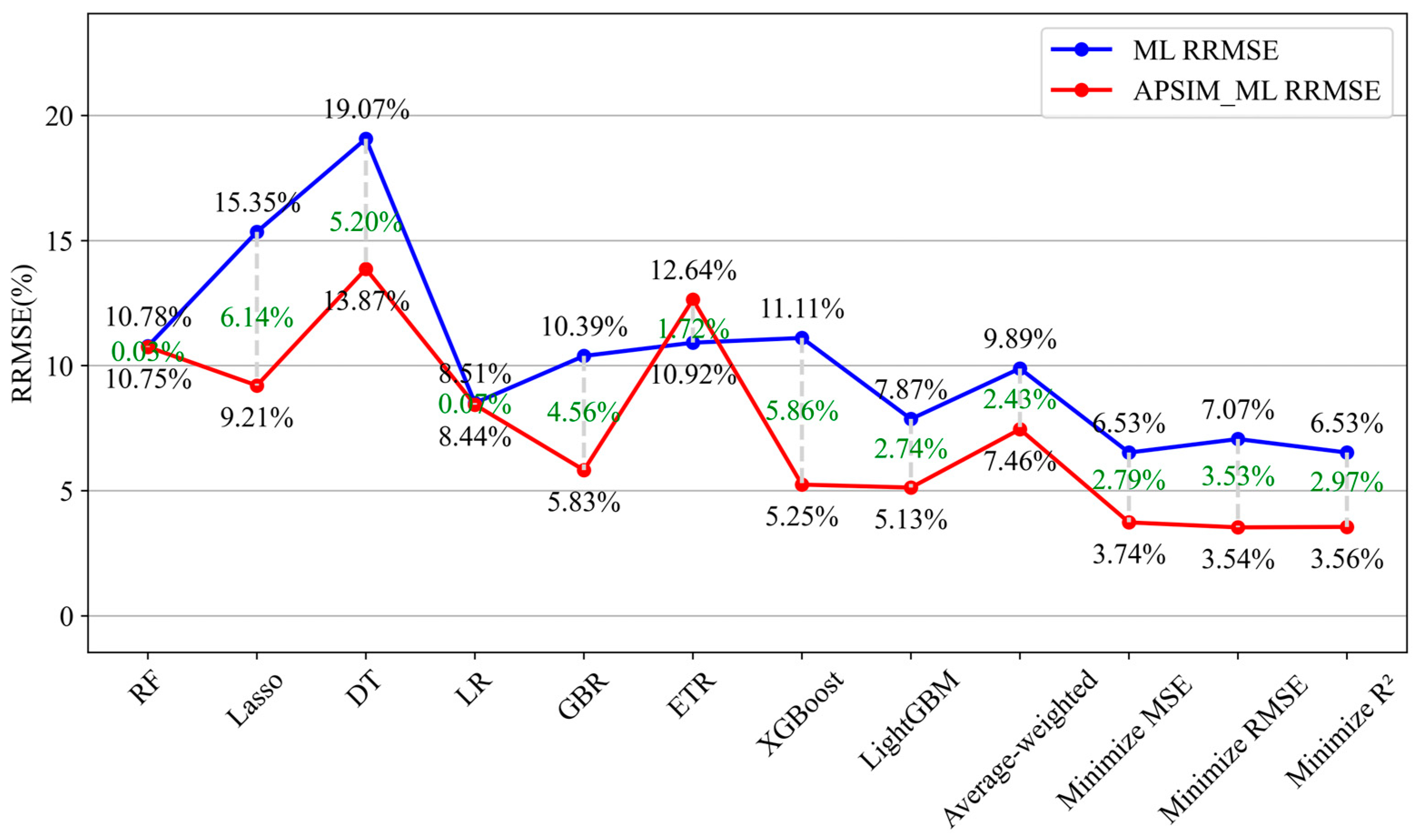
| ML Model | RMSE (kg/ha) | RRMSE (%) | MBE (kg/ha) | R2 | APSIM-ML Model | RMSE (kg/ha) | RRMSE (%) | MBE (kg/ha) | R2 | Increase in RRMSE (%) |
|---|---|---|---|---|---|---|---|---|---|---|
| Random Forest | 117.56 | 10.78 | −49.81 | 0.9718 | APSIM-Random Forest | 123.73 | 10.75 | 97.20 | 0.9684 | −0.03 |
| Lasso Regression | 166.21 | 15.35 | −41.83 | 0.9314 | APSIM-Lasso Regression | 106.89 | 9.21 | 78.55 | 0.9756 | −6.14 |
| Decision Tree | 209.03 | 19.07 | −21.97 | 0.8971 | APSIM-Decision Tree | 160.26 | 13.87 | 49.86 | 0.9453 | −5.2 |
| Linear Regression | 93.09 | 8.51 | −70.52 | 0.9846 | APSIM-Linear Regression | 98.07 | 8.44 | 57.45 | 0.9792 | −0.07 |
| Gradient Boosting | 114.01 | 10.39 | −25.4 | 0.9744 | APSIM-Gradient Boosting | 67.78 | 5.83 | 17.96 | 0.9902 | −4.56 |
| Extra Trees | 119.38 | 10.92 | −28.05 | 0.9661 | APSIM-Extra Trees | 146.34 | 12.64 | 116.25 | 0.9559 | 1.72 |
| XGBoost | 121.62 | 11.11 | −44.84 | 0.9643 | APSIM-XGBoost | 60.62 | 5.25 | 21.45 | 0.9921 | −5.86 |
| LightGBM | 85.56 | 7.87 | −34.98 | 0.9822 | APSIM-LightGBM | 58.36 | 5.1 | 17.28 | 0.9921 | −2.77 |
| Weighted Average Ensemble | 107.90 | 9.89 | −39.27 | 0.9701 | Weighted Average Ensemble | 86.56 | 7.46 | 56.88 | 0.9833 | −2.43 |
| Minimized MSE optimized weighted integrations | 70.07 | 6.53 | −11.71 | 0.9883 | Minimized MSE Optimized Weighted Integrations | 43.3 | 3.74 | −2.53 | 0.9957 | −2.79 |
| Minimized RMSE Optimized Weighted Integrations | 75.61 | 7.07 | −10.10 | 0.9852 | Minimized RMSE Optimized Weighted Integrations | 47.59 | 3.54 | 4.24 | 0.9953 | −3.53 |
| Minimized R2 Optimized Weighted Integrations | 70.94 | 6.53 | −8.34 | 0.9869 | Minimized R2 Optimized Weighted Integrations | 47.88 | 3.56 | 4.95 | 0.9950 | −2.97 |
Disclaimer/Publisher’s Note: The statements, opinions and data contained in all publications are solely those of the individual author(s) and contributor(s) and not of MDPI and/or the editor(s). MDPI and/or the editor(s) disclaim responsibility for any injury to people or property resulting from any ideas, methods, instructions or products referred to in the content. |
© 2024 by the authors. Licensee MDPI, Basel, Switzerland. This article is an open access article distributed under the terms and conditions of the Creative Commons Attribution (CC BY) license (https://creativecommons.org/licenses/by/4.0/).
Share and Cite
Li, Z.; Nie, Z.; Li, G. Integrating Crop Modeling and Machine Learning for the Improved Prediction of Dryland Wheat Yield. Agronomy 2024, 14, 777. https://doi.org/10.3390/agronomy14040777
Li Z, Nie Z, Li G. Integrating Crop Modeling and Machine Learning for the Improved Prediction of Dryland Wheat Yield. Agronomy. 2024; 14(4):777. https://doi.org/10.3390/agronomy14040777
Chicago/Turabian StyleLi, Zhiyang, Zhigang Nie, and Guang Li. 2024. "Integrating Crop Modeling and Machine Learning for the Improved Prediction of Dryland Wheat Yield" Agronomy 14, no. 4: 777. https://doi.org/10.3390/agronomy14040777
APA StyleLi, Z., Nie, Z., & Li, G. (2024). Integrating Crop Modeling and Machine Learning for the Improved Prediction of Dryland Wheat Yield. Agronomy, 14(4), 777. https://doi.org/10.3390/agronomy14040777