Evaluation of the Effect of Sentinel-1 SAR and Environmental Factors in Alfalfa Yield and Quality Estimation

Abstract

Alfalfa is one of the most widely cultivated perennial legume crops used as feedstock for animals. Efficiently estimating alfalfa yield and quality traits before harvesting is critical for the decision-making process regarding precision management activities and harvesting time to ensure high profitability. Satellite-based radar is a powerful tool in remote sensing for crop monitoring because it provides high-quality data regardless of weather conditions. Therefore, this study aims to investigate the potential use of satellite radar features and environmental factors in estimating alfalfa yield and quality. Alfalfa yield and quality traits, including dry matter yield (DMY), crude protein (CP), neutral detergent fiber (NDF), NDF digestibility (NDFD), and acid detergent fiber (ADF), were collected over 16 alfalfa fields from 2016 to 2021, leading to 126 samples in total. Sentinel-1 radar backscattering coefficients and environmental factors were collected for all the fields across all growing seasons. Five commonly used machine learning models were established to estimate each alfalfa trait separately. The results show that the Extreme Gradient Boosting model consistently performed the best for all alfalfa traits. The accuracy of the DMY estimates is acceptable, with an average R² of 0.67 and an RMSE of 0.68 tons/ha. The best result for estimating CP was an average R² of 0.70 and an RMSE of 1.63% DM. In estimating alfalfa fiber indicators (i.e., ADF, NDF, and NDFD), we achieved the highest average R² values of 0.54, 0.62, and 0.56, respectively. Overall, this study demonstrated the potential use of environmental factors for alfalfa yield and quality estimation in-field before harvesting. However, the Sentinel-1 radar backscattering coefficients did not make significant contributions to improving the estimation performance, compared to the environmental factors.

1. Introduction

Alfalfa, one of the most critical and stable legumes, is a valuable nutritious crop with a comparatively high yield, which is considered the fourth most valuable field crop in the United States behind corn, soybean, and wheat, and is a commercially grown source of forage and feed around the world [1,2]. In 2021 and 2022, 15.2 and 14.9 million acres were harvested, resulting in 49.2 and 47.9 million tons of alfalfa and alfalfa mixture for hay production in the United States, respectively [3]. Alfalfa is one of the most nutritive forages and is extensively applied as well-preserved forage in the diets of beef and dairy cattle [4,5,6]. The amount and quality of forage consumed by livestock are crucial to maintaining their health and milk production. Forage quality is regulated by two important components, including fiber (acid detergent fiber (ADF) and neutral detergent fiber (NDF)) and crude protein (CP). High-fiber alfalfa, with high fiber contents (ADF and NDF) and slow fiber digestibility (NDFD), results in rumen fill, which ultimately reduces energy intake and animal performance [5,7]. In addition, the concentration of protein, indicated by the CP, is also important, since amino acids from proteins are the building blocks for muscle, milk, and animal enzymes.

The proportions of fiber and CP in forage dry matter are dependent on the maturity stages when the forage is harvested. When alfalfa gets close to its maturity, the proportion of stems becomes greater relative to the leaves. As a result, the percentages of ADF and NDF increase relative to CP. As alfalfa quality traits and yield change rapidly during the short harvest window, the frequent and accurate estimation of alfalfa’s quality and yield becomes a critical issue in managing the tradeoff between yield and quality to obtain the highest total profits [8]. Alfalfa’s quantity and quality traits are traditionally determined by laboratory chemical methods, which are time-consuming, costly, labor-intensive, and can generate hazardous wastes [9]. Moreover, laboratory tests on a few samples are not sufficient to represent spatial variations within entire fields or those across a state and country. Recently, various remote sensing (RS) imaging platforms, such as unmanned aerial vehicles (UAVs) and satellites, have provided solutions for monitoring such crop traits over a variety of scales for different purposes [10,11,12].

UAV imagery has been widely used for crop monitoring due to its high spatial resolution as well as flexibility in temporal and spectral resolutions [13,14]. Its potential use in estimating alfalfa yield and quality traits has been evaluated with various UAV imagery, including hyperspectral images [8], digital image-based three-dimensional models [15], and aerial multispectral and thermal infrared images [16]. While the results are promising, UAV imagery has mainly been used to cover small-scale fields for applications in precision agriculture and breeding due to its limited payload and short flight endurance. In the previous studies, the covered area was limited to 0.2 [9] to 11 ha [15]. Therefore, UAV-based imagery is not applicable for monitoring alfalfa fields across a country or a state/province. Besides this, operating UAV platforms requires remote pilots with specific training and expertise. Daily data acquisition over large and multiple fields will significantly increase inputs of human labor and time, and thus the total costs. Plus, operating UAVs in mountainous locations is risky due to blocked signals, unexpected obstacles, and weather [17]. Consequently, relying on UAV imagery is impractical for informing alfalfa traits over large scales.

Satellite-based imagery has also been extensively investigated for use in agricultural crop monitoring. Compared to UAV imagery, satellite imagery benefits from its autonomy, accessibility, consistency, and scalability [18]. Satellites autonomously acquire data on large scales and in inaccessible mountainous areas, lowering the costs and risks of collecting RS data more than any other means. Moreover, satellite images, since launching, have been collected consistently around the Earth and securely stored, guaranteeing access to historical RS data over a region of interest. RS satellite-based optical and radar data are the two main types used for agricultural applications [19,20]. Among various satellite platforms, data from the optical platforms, e.g., Landsat-8, Sentinel-2, and Moderate Resolution Imaging Spectroradiometer (MODIS), have been investigated for use in estimating alfalfa yield. The Landsat-8 acquires multispectral data with a spatial resolution of 30 m in visible, near-infrared (NIR), and thermal infrared bands of electromagnetic waves, providing valuable observations for crop monitoring at the field and county levels. Kayad et al. investigated the correlation between a few vegetation indices (VIs) derived from the Landsat-8 Level 1 GeoTIFF data products and alfalfa yield measured by a hay yield monitoring system on a rectangular baler [11]. The highest corresponding correlations of determination (R²) of 0.54, 0.56, and 0.53 were obtained for the linear regressions between alfalfa yield and NIR, Soil Adjusted VI (SAVI) and Normalized Difference VI (NDVI), respectively. Moving beyond the investigation of linear correlations, Azadbakht et al. adopted machine learning methods for estimating alfalfa yield using time-series image features from Landsat 8 and PROBA-V. The best estimation performance was achieved by the Gaussian Process Regression (GPR) model with an R² of 0.92 and RMSE of 1.1 tons/ha with the selected time-series features over three years [10]. Similarly, He et al. used features from both MODIS and Landsat imagery as inputs to the data-driven light use efficiency (LUE) model for estimating county-level alfalfa yield, and achieved an R² of 0.72 between the estimated and measured values [21]. Interestingly, Sadenova et al. compared the performance in forecasting alfalfa yield at the field level among satellite, UAV, and weather data. It was found that the best result (R² = 0.94 and RMSE = 0.25 t/ha) was given by the Random Forest (RF) model with a combined input dataset of image features from both UAV and satellites (Sentinel-2, Landsat-8, and MODIS) with climatic and weather data, showing the improvement achieved by combining remote sensing data with environmental information [22].

Although demonstrated in previous studies to show promising performance, success in crop monitoring on particular regions could be limited when solely relying on satellite optical data because areas at high latitudes on Earth are severely affected by cloud, fog, and evaporation, resulting in up to 80% being missing for those areas [23,24]. Instead, RS radar-based satellites could be effectively applied in these areas as they function by transmitting and receiving electromagnetic waves in microwave ranges, including Ku (1.6–2.5 cm), X (2.5–3.75 cm), C (3.75–7.5 cm), L (15–30 cm), and P (30–130 cm) bands, which are nearly unaffected by clouds due to their long wavelength [25]. Therefore, radar data have received special attention for use in crop monitoring at high latitudes due to their capacity to acquire data regardless of the weather and external energy sources, such as the Sun or the energy radiation of the objects [19,20]. Synthetic aperture radar (SAR) satellites, a form of radar satellites, collect data with a finer spatial resolution by utilizing the synthetic aperture antenna for capturing data from the target. Sentinel-1 is a combination of two satellites deployed by the European Space Agency in 2014 and 2015, providing C-band SAR data with a spatial resolution of 5 m in range and 20 m azimuth in Interferometric Wide Swath mode (IW mode) [26]. Sentinel-1 provides free and high-resolution SAR backscattering coefficients, which have been recently used for a variety of crop monitoring purposes, including aboveground biomass (AGB), height, and leaf area index in large pasture fields [27]; quantity and quality of semi-natural grassland forage [28]; and biophysical parameters of wheat, soybeans, and canola [29]. However, there are no studies reported on estimating alfalfa yield using satellite radar data, nor on estimating alfalfa quality traits using any satellite features [30].

Beyond remote sensing data, numerous studies have also utilized environmental data to estimate the yield and quality of alfalfa [31], especially regarding factors like light duration [32], water [33], and temperature [34]. Besides directly using temperature data, the application of Growing Degree Days (GDD) for evaluating yield and quality has seen widespread use [1,35]. Given the diversity of experimental setups, the response of yield and quality traits to environmental factors varies greatly across studies. For example, moisture can significantly affect alfalfa yield [36], or it may show no clear trend [37]. Therefore, analyzing a single factor is not comprehensive enough; the combined impact of different environmental factors is an indispensable aspect that must be considered for an accurate estimation. To date, studies solely utilizing environmental factors are rare; a multi-factor combination, especially in conjunction with remote sensing data, can achieve higher precision [1]. The majority use optical remote sensing data, which, despite their susceptibility to weather impacts, do not align well with the stable data acquisition capacities of environmental data. Hence, combining environmental data with stably acquired SAR imagery could further validate the potential for long-term stable monitoring.

Therefore, this study aims to investigate the potential of two types of stably acquired data, satellite radar data (Sentinel-1) and environmental factors, in estimating alfalfa DMY and quality traits. For this purpose, the objectives are itemized as follows: (1) evaluating the significance of SAR data and environmental factors in explaining the variations of alfalfa DMY and quality traits; (2) evaluating the performance in estimating alfalfa yield and quality traits using Sentinel-1 SAR features and environmental factors; (3) comparing the estimation accuracy for each of the alfalfa traits among machine learning models.

2. Materials and Methods

The workflow of this study is illustrated in Figure 1. The first step involves collecting samples from the experimental fields for yield and quality analysis, as well as acquiring satellite and environmental data. The features calculated from these data are statistically analyzed and used as input features for the machine learning (ML) models. Through strategies such as cross-validation and feature combination, the evaluation accuracy of different features is analyzed. Finally, the optimal model is used to generate alfalfa yield and quality maps.

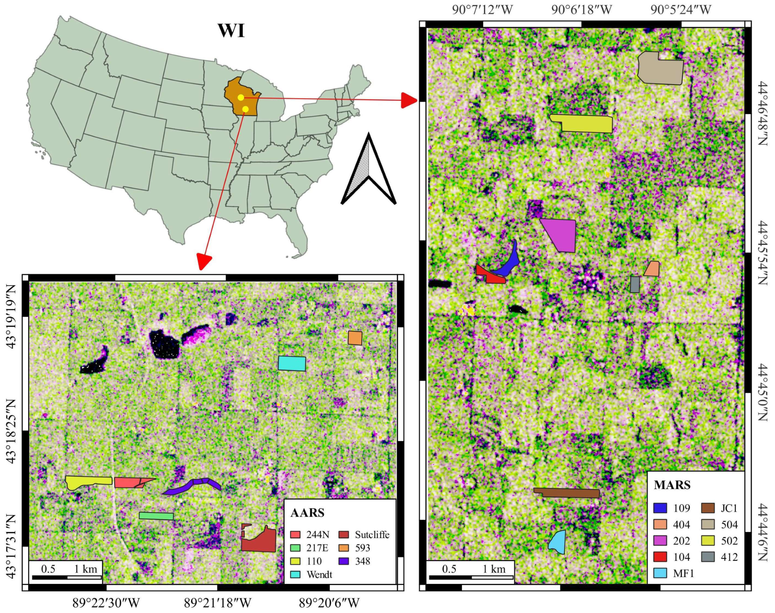
2.1. Study Area and Ground Data Sampling

The study was conducted from 2013 to 2021 at the Arlington Agricultural Research Station (AARS, latitude of 43°16′ N to 43°20′ N and longitude of 89°19′ W to 89°24′ W) and Marshfield Agricultural Research Station (MARS, latitude of 44°43′ N to 44°48′ N and longitude of 90°04′ W to 90°08′ W) at the University of Wisconsin-Madison. From 2016 to 2021, ground data (i.e., alfalfa DMY, CP, ADF, NDF, and NDFD) were collected from seven sites at AARS and nine sites at MARS. The geographic locations of the research stations and the distribution of the sampling sites are shown in Figure 2. Alfalfa in each site was sampled three to four times in each growing season starting from the first year and extending to three years after seeding. The detailed sampling times for all the sites are listed in

Table 1. Sampling sites and times.

Site ID	Year Seeded	Alfalfa Variety	Sampling Years
AARS-593	2013	Pioneer 55V50	2016 (4), 2017 (4)
AARS-348	2014	Mixed RR varieties	2016 (4), 2017 (4), 2018 (4)
AARS-217E	2015	Pioneer 55V50/Dairyland HF3400	2016 (4), 2017 (4), 2018 (4)
AARS-244N	2016	HVXRR 4.0 Brand	2017 (4), 2018 (4), 2019 (4)
AARS-Wendt	2017	Pioneer 55VR08	2018 (4), 2019 (4), 2020 (4)
AARS-110	2018	Jung 4R418	2019 (4), 2020 (4), 2021 (4)
AARS-Sutcliffe	2019	HybriForce 3431	2020 (4), 2021 (4)
MARS-109	2014	Dairyland Magnum 7/wet	2016 (3), 2017 (4)
MARS-JC1	2015	Dairyland Magnum 7/wet	2016 (3), 2017 (3)
MARS-404	2016	Dairyland Hybriforce 3405	2017 (3), 2018 (4)
MARS-504	2016	Dairyland 2420/wet	2017 (3), 2018 (4)
MARS-MF1	2017	Dairyland 3420/wet	2018 (4), 2019 (3)
MARS-202	2018	Dairyland 3420/wet	2019 (4), 2020 (4)
MARS-502	2018	Dairyland 3420/wet	2019 (4)
MARS-412	2016	Pioneer 55V50	2016 (1)
MARS-104	2019	Dairyland 3420/wet	2020 (3)

. The first cut (sampling) of individual sites in a year usually happened at the end of May; there was a roughly one-month interval between two cuts. Therefore, the second, third, and fourth cuts happened at the end of June, July, and August, respectively. In total, 126 samples were collected for measuring alfalfa DMY and quality traits, categorized by the sites, years, and cutting orders. Due to the limited and uneven numbers of samples for each alfalfa variety, we did not discuss them separately in the subsequent analysis, and treated the variety as a random factor.

The total wet yield of each experimental site was obtained during the harvest by weighing the empty and full trucks carrying the harvested forage with an on-farm drive-over scale [38]. The total dry yield was then obtained by multiplying the total wet yield by a dry/wet ratio obtained using two dried samples that were randomly selected from each harvest. Then, the DMY of a field was taken as the total dry yield divided by its size. The two selected samples were then sent to the UW Soil & Forage Analysis Laboratory (https://uwlab.soils.wisc.edu/, accessed on 13 April 2024) for quality analysis of CP, ADF, NDF, and NDFD). The CP and ADF were analyzed by Near Infrared Reflectance Spectroscopy (NIRS), while the NDF and NDFD were tested through wet chemistry analysis. The results from the two forage samples were averaged for each harvest [38].

Major environmental factors (Figure A1 and Figure A2 in Appendix A) during alfalfa regrowth were collected from Daymet V4 [39], including the daylight duration (period of days during which the sun is above a hypothetical flat horizon), precipitation, incident shortwave radiation flux density or radiation for short (taken as an average over the daylight period of the day), and vapor pressure (VP, daily average partial pressure of water vapor). GDD was calculated to assess crop development over the regrowth period, using Equation (1). We used the cumulative values of each environmental factor over the regrowth before each cut (around one month period) as input variables for further analysis. For the first cut in a year, we calculated the cumulative values from 30 days prior to the cut to the day before the cut, and for the second to fourth cut, we calculated the cumulative values from the day after the previous cut to the day before the current cut.

$$GDD=(T_{max}+T_{min})/2-T_{base}$$

(1)

where $T_{max}$ and $T_{min}$ are the maximum and minimum air temperature in a day. $T_{base}$ was set to 5 °C [40,41].

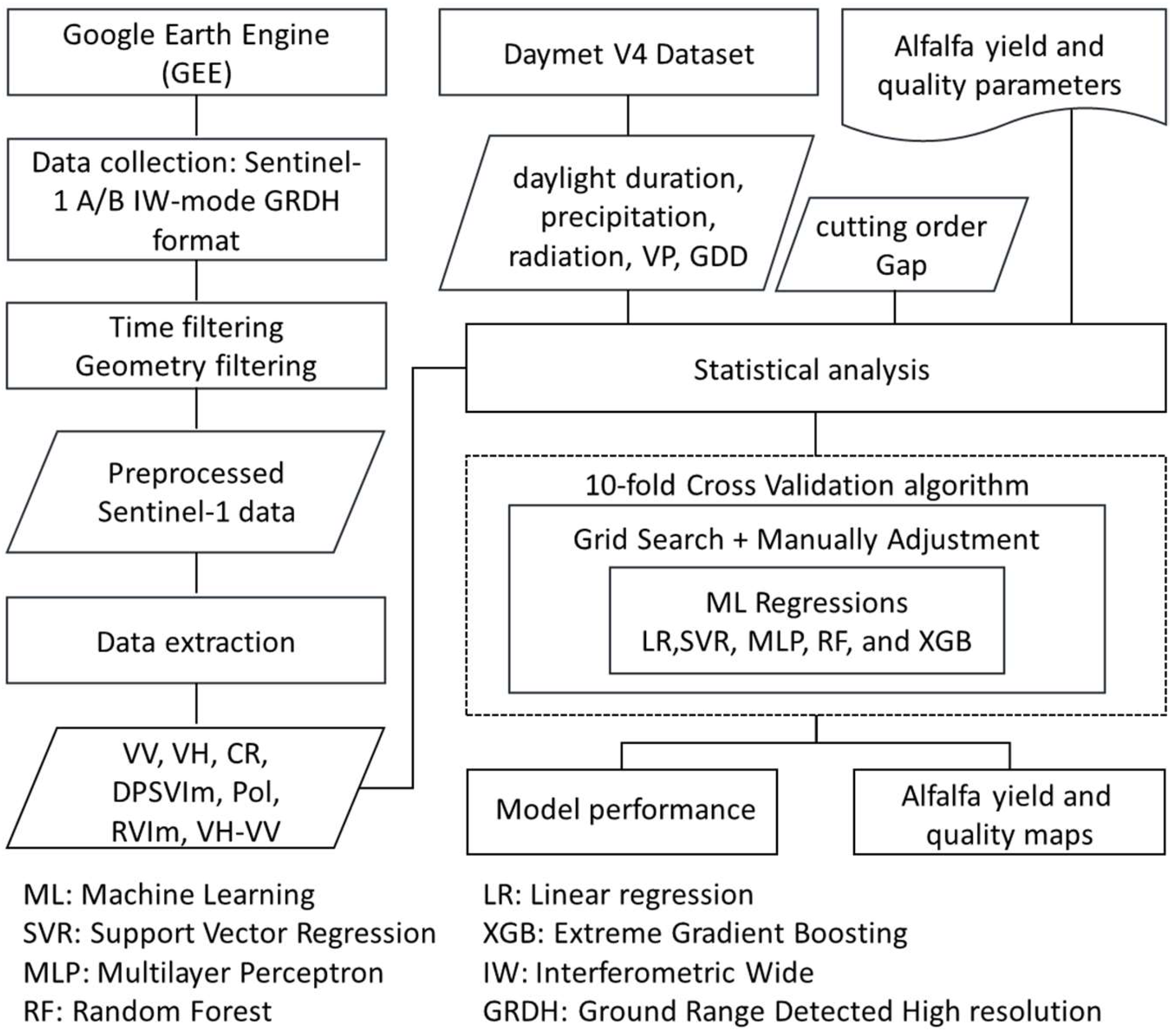
2.2. Satellite Image Acquisition and Processing

Sentinel-1 imagery over all the experimental sites from 2016 to 2021 was acquired and processed for estimating alfalfa DMY and quality traits. Technically, the two polar-orbiting satellites (Sentinel-1 A and B) provide imagery with a six-day temporal resolution. However, the six-day resolution is mainly ensured over Europe, while 1–12-day revisit circles are expected for other parts of the world. In this study, features at two acquisition dates were processed for each sample, namely, the late features (from the closest imaging day to the ground sampling date) and the early features (from the second-closest imaging day to the ground sampling date). The SAR data were collected from the high-resolution Ground Range Detected (GRD) products of Sentinel-1 in the IW mode.

As shown in Figure 1, the GRD images were downloaded using the Google Earth Engine (GEE) cloud platform and preprocessed using the Sentinel-1 toolbox [36] provided by the European Space Agency. These data have been preprocessed in five steps: (1) applying orbit file, (2) GRDH border noise removal, (3) thermal noise removal, (4) radiometric calibration computing backscatter coefficients using sensor calibration parameters in the GRD metadata, and (5) terrain correction. The SAR images were then reshaped to a 30 m spatial resolution with the nearest approach. Backscattering coefficients VV (${\sigma }_{VV}^o$) and VH (${\sigma }_{VH}^o$), along with the cross-polarization ratio or CR (${\sigma }_{VV}^o$/${\sigma }_{VH}^o$), modified Dual Polarization SAR Vegetation Index or DPSVIm ((${\sigma }_{VV}^o\ast {\sigma }_{VV}^o$+${\sigma }_{VH}^o\ast {\sigma }_{VV}^o$)/$\sqrt{2}$) [42], normalized polarization or Pol ((${\sigma }_{VH}^o-{\sigma }_{VV}^o)$/${(\sigma }_{VH}^o+{\sigma }_{VV}^o$)) [43], modified Radar Vegetation Index or RVIm ((${4\ast \sigma }_{VH}^o)$/${(\sigma }_{VH}^o+{\sigma }_{VV}^o$)) [44], and VH-VV (${\sigma }_{VH}^o-{\sigma }_{VV}^o$), were calculated and used as input features to estimate the alfalfa DMY and quality traits. Each sample was featured with a Gap variable, indicating the day difference between when the sample was cut and when it was imaged (the satellite acquisition dates). To increase the sample size for machine learning modeling, we resampled the dataset by stacking samples with early features and late features and removed those that were imaged too long ago from the sampling days (i.e., Gap > 12 days), leading to a dataset with 216 samples for training and validating the machine learning models.

2.3. Statistical Analysis and Machine Learning Modelling

Statistical analysis and machine learning modeling were performed in Python (Version 3.11.4). A two-way analysis of variance (ANOVA) was conducted to evaluate the effects of cutting orders, environmental factors and SAR image features on alfalfa DMY and quality traits and the explained variations in alfalfa traits by combining environmental factors and SAR features. The ANOVA tests were conducted at a significance level of 5% using the “aov” function. In the first ANOVA test with only the cutting orders and environmental factors as variables, we assumed an interaction between the cutting orders and each of the environmental factors (daylight duration, precipitation, radiation, GDD, and VP), while in the second ANOVA test, the SAR image features and Gap were added with the consideration of an interaction between the cutting orders and each of the image features. The explained variation of each variable was calculated as the percentage of the sum of squares regression (SSR) of the variable in the sum of squares total (SST) in the test. A p-value indicating whether the variable has a significant effect on alfalfa traits has also been reported.

To evaluate the performance of machine learning models in estimating alfalfa DMY and quality traits, five models that have been widely used in estimating crop traits with remote sensing data, namely, Linear Regression (LR), Support Vector Regression (SVR), Multilayer Perceptron (MLP), Random Forest (RF), and Extreme Gradient Boosting (XGB), were developed and validated using the dataset. Optimal hyperparameters in each non-linear model were found for each alfalfa trait using a grid search algorithm. The search range and steps for all the hyperparameters are listed in

Table 2. Grid search specifications for hyperparameters of the machine learning models.

Model	Hyperparameter	Searching Range
SVR	Squared L2 penalty	0.01, 0.1, 0.5, 1, 5, 10, 100
	Gamma	0.01, 0.1, 0.5, 1, 5, 10, 100
MLP	Activation	‘identity’, ‘logistic’, ‘tanh’, ‘relu’
	Solver	‘adam’, ‘sgd’
	Hidden layers	10, 15, 20, 25, 30, 35, 40
	Batch size	20, 24, 32, 40
	Random state	0, 1, 2, 3
RF	Max features	‘sqrt’, ‘log2’, 0.3, 0.5, 1
	Number of trees	30, 40, 50, 80, 100
	The minimum samples at leaf	2, 4, 6, 8, 10
	Random state	0, 1, 2, 3
XGB	Maximum depth	3, 4, 5, 6, 7, 8
	Number of trees	30, 40, 50, 80, 100
	Learning rate	0.01, 0.05, 0.1
	Tree method	‘exact’, ‘approx’, ‘hist’
	L1 regularization	0.4, 0.5, 0.8, 1
	L2 regularization	0.6, 0.8, 1, 1.2

, as well as their optimized values. The model performance was evaluated using ten-fold cross-validation (CV), which was repeated for each alfalfa trait 20 times. In each of the repetitions, the coefficient of determination (R²), root mean square error (RMSE) and mean absolute error (MAE) were calculated between the estimated and measured values. Averages of the three metrics over the 20 CV repetitions are reported.

3. Results and Discussion

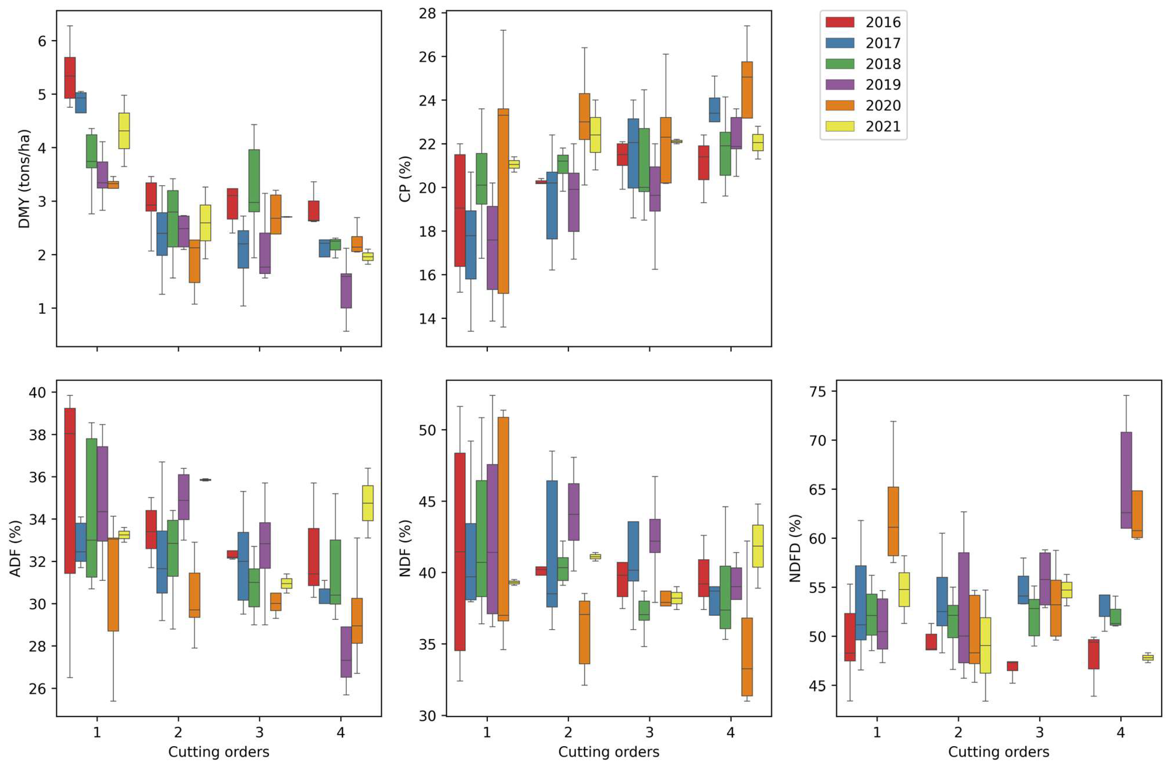
3.1. Ground Data Statistics

Distributions of DMY and quality traits for alfalfa harvested in each year from 2016 to 2021 are plotted against the cutting orders in Figure 3. The DMY decreased with increasing cutting order in all years, with the first cut yielding significantly higher than each of the others. This is because the growth duration for the first cut of alfalfa was significantly longer than the others, from the end of the last season (September) to May of the next year, allowing more biomass accumulation [4,45]. Besides this, when alfalfa plants were cut, they utilized the stored energy reserves in their roots to regrow and produce new shoots. Multiple cuts in a growing season led to a gradual decrease in these energy reserves, reducing the plant’s ability to produce as much dry matter in subsequent cuts [46]. Moreover, changes in environmental conditions, such as temperature, precipitation, and radiation duration, could jointly impact the plant’s ability to produce dry matter in subsequent cuts. While the DMYs of the second cuts were relatively stable over the years, the third cuts had a trend of DMY increase, with high variation. In some years (e.g., 2016, 2018, and 2020), the third cuts yielded more than the second cuts, while in some years (e.g., 2017 and 2019), they were much lower. These variations could have been caused by the weather changes in the month.

Increasing trends in the CP content with narrower ranges can be observed throughout successive cuts in Figure 3. While the general trend in the previous studies suggests a decline in alfalfa CP content with successive cuts, variabilities in alfalfa varieties and growing environments in this dataset could contribute to the opposite pattern. Growth patterns and responses to cutting varied among alfalfa varieties, with some producing higher protein content during later regrowth stages and others lower. Besides this, the ability to synthesize protein from outside nitrogen from the atmosphere and soil highly depends on soil fertility, environmental conditions, management practices, and previous cutting schedules [47,48]. Variations in these factors and their interactions introduced large variabilities in estimating CP from this dataset.

The ADF, NDF, and NDFD remained around similar levels from the first to the last cut, without a significant decrease or increase noticed. Low fiber contents represent better alfalfa quality, as they ensure the sufficient nutritional intake of dairy cows and consequently result in increased milk protein and production [4,5]. Alfalfa with high fiber contents and a low concentration of protein does not support an adequate supply of metabolizable protein, and reduces energy intake and animal performance as a result of faster rumen fill, resulting in a reduction in milk production [49]. However, it is important to note that there are a few factors interacting with each other and the cutting time, consequently affecting the ADF and NDF content in alfalfa productions with temporal and geographic variations, including harvest timing, environmental factors, soil fertility and nutrient availability, varietal differences, and stressors [50]. Thus, strategically taking these factors into consideration plays an important role in estimating alfalfa fiber contents.

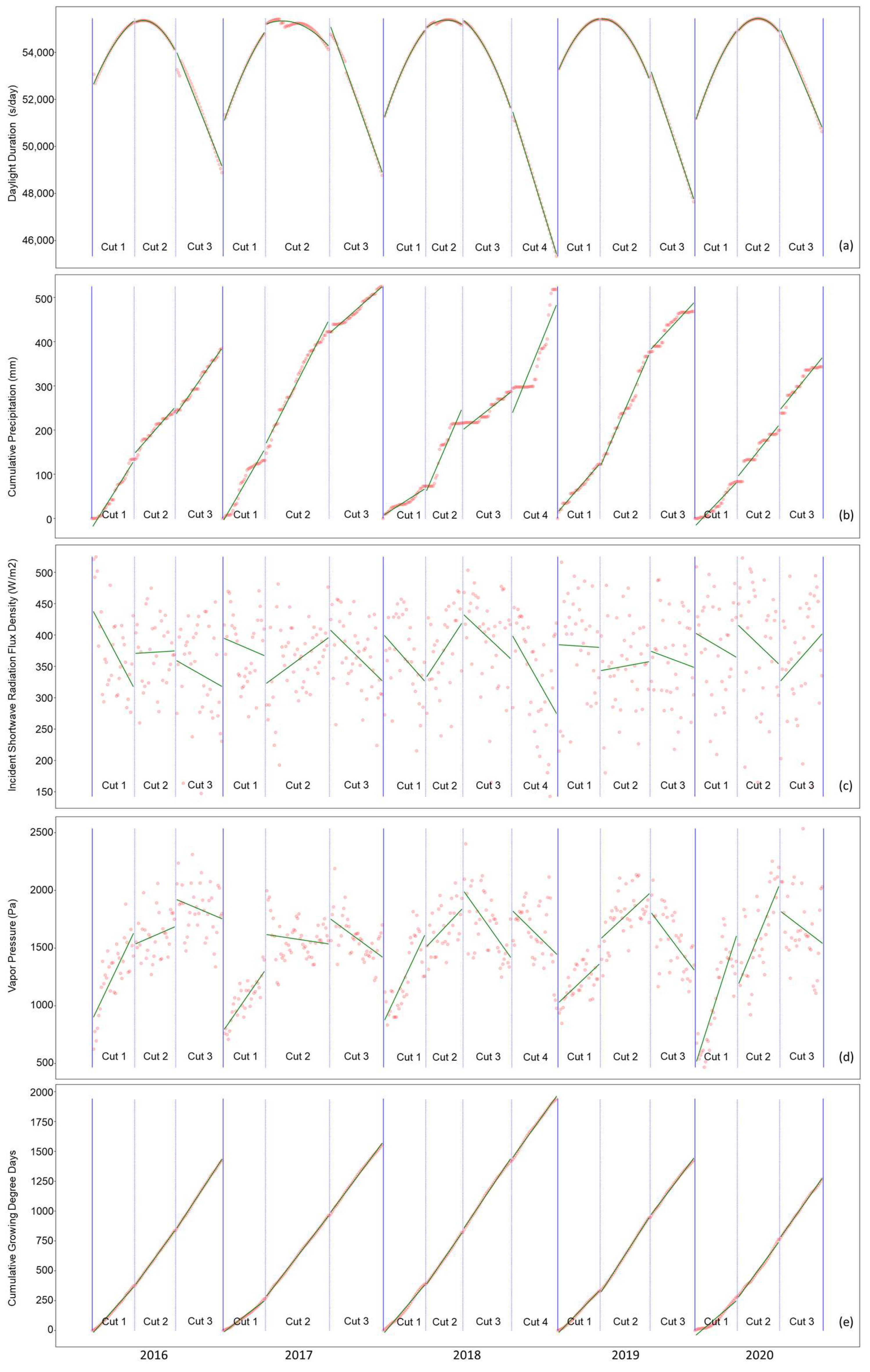
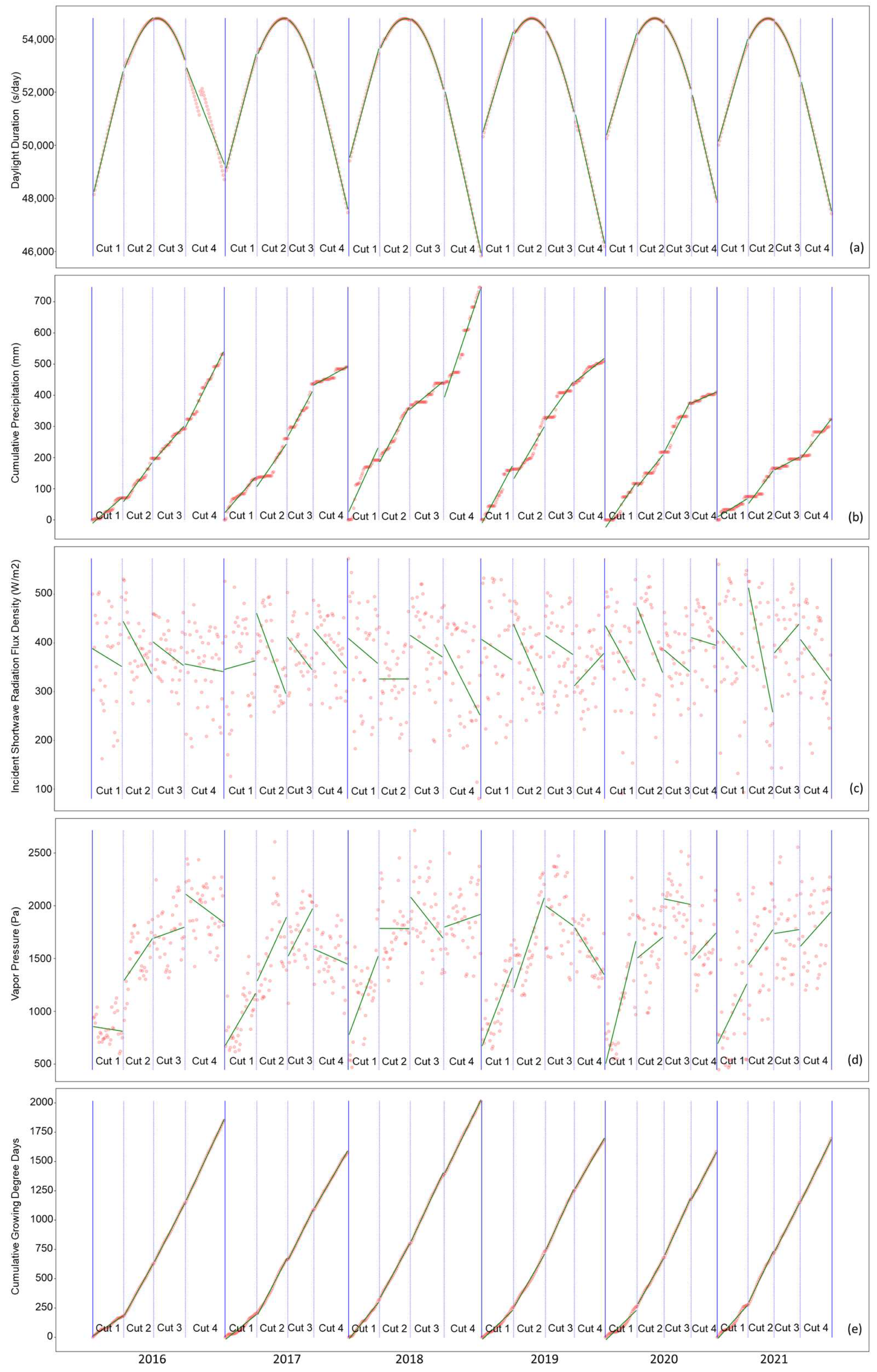
3.2. Variations in Alfalfa DMY and Quality Traits Explained by Environmental Factors and Image Features

Variations among alfalfa DMY and quality traits explained by the cutting order and weather data in the ANOVA are listed in

Table 3. Variations in alfalfa DMY and quality traits explained by only the weather data in two-way ANOVA.

	DMY	CP	ADF	NDF	NDFD
Cutting orders	30.78 ***	6.35 ***	14.93 ***	10.97 ***	11.67 ***
Daylight duration	0.27 NS	3.02 ***	2.04 NS	2.44 ***	1.01 NS
Precipitation	1.88 NS	18.14 ***	6.75 ***	7.38 ***	2.50 NS
Radiation	0.68 NS	0.98 NS	1.06 NS	0.39 NS	0.02 NS
GDD	3.86 NS	6.99 ***	1.15 NS	3.57 NS	6.73 ***
VP	2.35 ***	1.41 ***	2.94 ***	1.14 NS	3.56 ***
Cutting orders: daylight duration	1.88 NS	5.71 ***	2.62 NS	2.62 NS	3.39 NS
Cutting orders: precipitation	1.28 NS	1.45 ***	7.04 ***	2.73 ***	3.38 ***
Cutting orders: radiation	2.08 NS	9.59 ***	1.81 NS	5.73 ***	6.15 ***
Cutting orders: GDD	0.28 NS	1.16 NS	3.24 ***	1.19 NS	1.58 NS
Cutting orders: VP	2.97 NS	11.69 ***	2.25 NS	4.81 ***	4.98 ***
Error	51.67	33.52	54.17	57.04	55.02

Numbers in the table are presented in percentages. *** indicate the significance levels of p = 0.001, respectively. NS stands for no significance.

. The variations could be explained by the input variables of 48.33%, 66.48%, 45.83%, 42.96%, and 44.98% for the DMY, CP, ADF, NDF, and NDFD, respectively. The cutting order has a significant effect on all the alfalfa traits. Particularly, it explained over 30% of the variation in the alfalfa DMY, which confirms the observations in Figure 3. Other than the cutting order, the VP also significantly relates to the alfalfa DMY. No interaction effects were noticed between cutting order and weather conditions on DMY, which implies that the effects of weather conditions on alfalfa DMY remained unchanged among different cuttings. The CP was also significantly affected by daylight duration, precipitation, GDD, and VP. Moreover, the interaction between cutting order and weather conditions (except for the GDD) was also significant, indicating the extent to which weather conditions affect alfalfa CP depending upon the regrowth stages in a season. While the radiation had no significant effect on all three fiber contents, the daylight duration had a significant effect on the NDF, the precipitation had a significant effect on the ADF and NDF, VP had a significant effect on both ADF and NDFD, and GDD only affected NDFD. It was also noted that the interaction between cutting order and precipitation was also significant for all three fiber contents, implying that the fiber formation relates to the water availability in summer during regrowth.

Variations among alfalfa DMY and quality traits explained by the cutting order, weather data, and SAR features are listed in

Table 4. Variations in alfalfa DMY and quality traits explained by weather data and SAR features in two-way ANOVA.

	DMY	CP	ADF	NDF	NDFD
Cutting orders	26.00 ***	10.31 ***	15.11 ***	17.22 ***	12.81 ***
Daylight	0.79 NS	1.96 *	0.98 NS	0.85 NS	1.05 NS
Precipitation	0.94 NS	2.12 *	0.78 NS	0.36 NS	0.04 NS
Radiation	2.18 *	0.54 NS	0.84 NS	0.39 NS	1.04 NS
GDD	1.91 *	1.70 NS	4.64 *	1.86 NS	3.18 ***
VP	0.83 NS	1.64 NS	2.51 NS	0.56 NS	2.27 NS
Cutting orders: daylight	2.89 NS	14.23 ***	4.67 NS	4.99 NS	2.46 NS
Cutting orders: precipitation	3.73 NS	5.21 *	1.36 NS	3.11 NS	5.07 NS
Cutting orders: radiation	2.91 NS	4.96 *	2.08 NS	3.08 NS	1.05 NS
Cutting orders: GDD	1.59 NS	6.79 **	1.44 NS	3.97 NS	7.27 ***
Cutting orders: VP	2.53 NS	8.61 **	1.42 NS	2.83 NS	4.50 NS
Gaps	0.04 NS	0.05 NS	0.15 NS	0.44 NS	0.50 NS
VV	3.43 ***	0.02 NS	0.28 NS	0.10 NS	0.02 NS
VH	3.44 ***	0.02 NS	0.28 NS	0.10 NS	0.02 NS
CR	1.20 NS	0.07 NS	1.20 NS	0.13 NS	3.40 ***
DPSVIm	0.22 NS	0.00 NS	0.04 NS	0.34 NS	0.11 NS
Pol	0.08 NS	0.53 NS	0.01 NS	0.25 NS	0.18 NS
RVIm	0.26 NS	0.00 NS	0.06 NS	0.30 NS	0.14 NS
VH-VV	3.44 ***	0.02 NS	0.28 NS	0.10 NS	0.02 NS
Cutting orders: VV	1.40 NS	1.45 NS	1.79 NS	1.80 NS	0.10 NS
Cutting orders: VH	1.39 NS	1.45 NS	1.80 NS	1.80 NS	0.10 NS
Cutting orders: CR	0.43 NS	0.42 NS	0.63 NS	1.57 NS	0.43 NS
Cutting orders: DPSVIm	0.28 NS	0.37 NS	3.20 NS	1.39 NS	0.57 NS
Cutting orders: Pol	3.06 NS	0.77 NS	0.49 NS	2.96 NS	1.69 NS
Cutting orders: RVIm	0.31 NS	0.37 NS	3.23 NS	1.43 NS	0.58 NS
Cutting orders: VH-VV	1.39 NS	1.45 NS	1.80 NS	1.80 NS	0.10 NS
Error	33.32	34.96	48.95	46.26	51.33

Numbers in the table are presented in percentages. *, **, *** indicate the significance levels of p = 0.05, 0.01 and 0.001, respectively. NS stands for no significance.

. With the addition of SAR features, the explained variations in DMY, ADF, NDF, and NDFD were improved to 66.68%, 51.05%, 53.73%, and 48.67%, respectively. For the DMY, VV, VH, and VH-VV had significant effects, but their interaction with the cutting order did not. This implies that the effect on DMY of these features remained consistent during the different regrowth stages. Among the fiber contents, NDFD is the only one that has been significantly affected by the SAR feature CR. Although the explained variations were increased in ADF and NDF, none of the SAR features had significant effects. Comparing these results to those in Table 3, it can be seen that the SAR features help with explaining some of the variations in alfalfa DMY and fiber contents that were not explained by the weather data alone in the ANOVA analysis. The remaining variations could have been caused by other factors that were considered random in this analysis, such as soil type, fertilizer application, and pest management, or could be captured by the linear relationship. Therefore, in the following sections, we will evaluate the performance of ML models in representing and estimating alfalfa DMY and quality traits.

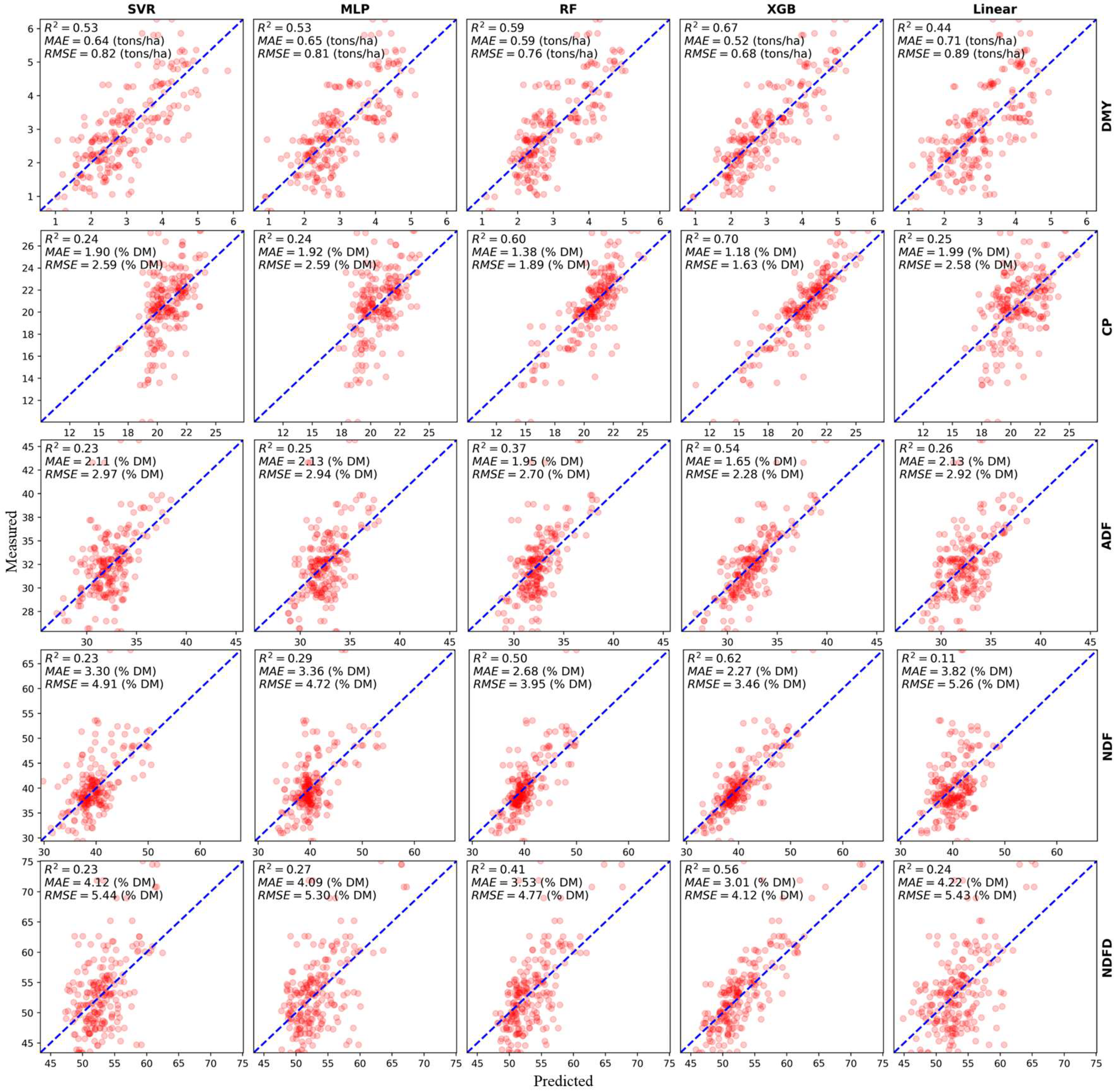
3.3. Performance for Alfalfa DMY and Quality Traits

Figure 4 shows scatterplots between the alfalfas’ measured and estimated values given by the five trained models. The DMY estimates given by the XGB models closely agree with the measured values, with an average R² of 0.67 and RMSE of 0.68 tons/ha over the 20 repeated CV. The models’ performances benefited from the relationships between either DMY or backscattering coefficients and vegetation water content (VWC). DMY, though measured as the weight of water-free substances in vegetation samples, has a high correlation with the VWC. Zhou et al. and Bhattacharya showed a strong linear relationship (r = 0.96) between DMY and VWC [51,52]. Logically, vegetation with more water has a higher capacity to sustain water, supported by a larger volume of dry matter. On the other hand, radar backscattering coefficients from vegetation are highly related to the VWC because water absorbs more energy than other substances in vegetation [20,53,54]. Consequently, vegetations with higher VWC tend to reflect fewer radar signals than those with lower VWC.

Our results are competitive compared to previous studies using satellite optical data. Azadbakht et al. reported an R² of 0.92, an RMSE of 1.1 tons/ha, and an MAE of 0.8 tons/ha using the GPR model with the selected time-series Landsat 8 and PROBA-V features [10]. Using single-time satellite SAR data requires less data processing and computational effort, while achieving lower average errors. The best results in estimating alfalfa DMY described in the published literature were an R² = 0.94 and RMSE = 0.25 t/ha, reported by [22], which, however, required high-resolution images from UAV as well as satellite imagery from three platforms (i.e., Sentinel-2, Landsat-8, and MODIS). Overall, the performance of this study suggests its practical use in estimating alfalfa DMY.

For estimating CP, the best result, with an average R² of 0.70 and RMSE of 1.63%, was given by the XGB model (Figure 4). The CP concentration in alfalfa is related to chlorophyll concentration, which is closely dependent on its water and nitrogen status [28]. Therefore, it could be reflected by the backscattering coefficients. The CP estimates agree the most with the measured values in our studies, demonstrating its utility in practical use [15,19,28]. The performances in estimating alfalfa fiber indicators (i.e., ADF, NDF, and NDFD) are shown in Figure 4, with the highest average R² values of 0.54, 0.62, and 0.56, respectively. The best estimates for the three fiber indicators were all given by the XGB models. The relationships between backscattering coefficients and plant density account for the models’ performance. Plant density primarily affects the structure of the plant population. Increasing plant density causes more competition among individuals for nutrients, water, and light, and consequently lowers the quality by increasing fiber contents in the plant. It was reported that the fiber contents (ADF and NDF) increased with higher plant densities, thus resulting in decreasing quality [55,56,57,58]. In addition to VWC, radar backscattering coefficients from vegetation are affected by geometric factors including plant density, pattern, and height. Dense and high objects increase both the duration and energy of radar signals being reflected to the satellite receiver, accordingly resulting in higher backscattering coefficients [25,59,60,61].

3.4. Impact of Environmental Factors and SAR Features on Estimates

To investigate the impact of environmental factors and SAR features on yield and quality estimation, it is crucial to avoid the errors caused by repeated environmental factors in the expanded dataset. Therefore, we conducted experiments with 117 samples from the original dataset with a gap less than 12 days to demonstrate the contributions of these two types of features.

Table 5. Performances of the five machine learning models in estimating alfalfa yield and quality traits.

Input	Traits	SVR			MLP			RF			XGB			LR
		R2	RMSE	MAE	R2	RMSE	MAE	R2	RMSE	MAE	R2	RMSE	MAE	R2	RMSE	MAE
Group 1	DMY	0.51	0.82	0.64	0.46	0.84	0.69	0.41	0.89	0.72	0.28	0.99	0.77	0.34	0.94	0.77
	CP	0.39	2.28	1.70	0.20	2.61	1.91	0.42	2.22	1.68	0.39	2.29	1.75	0.20	2.61	1.97
	ADF	0.25	2.92	2.13	0.15	3.10	2.27	0.19	3.04	2.31	−0.01	3.38	2.53	0.19	3.03	2.25
	NDF	0.35	4.48	3.14	0.21	4.91	3.51	0.32	4.57	3.23	0.20	4.94	3.51	0.13	5.16	3.75
	NDFD	0.21	5.60	4.16	0.06	6.08	4.57	0.17	5.72	4.29	0.18	5.68	4.27	0.10	5.97	4.70
Group 2	DMY	0.40	0.89	0.72	0.43	0.89	0.72	0.42	0.89	0.72	0.33	0.94	0.74	0.37	0.91	0.77
	CP	0.24	2.55	1.90	0.23	2.57	1.93	0.21	2.60	1.95	0.06	2.84	2.18	0.16	2.67	2.01
	ADF	0.12	3.15	2.39	0.11	3.17	2.40	0.08	3.23	2.41	−0.08	3.49	2.63	0.02	3.33	2.54
	NDF	−0.01	5.58	3.90	−0.04	5.65	3.94	0.05	5.41	4.01	−0.27	6.23	4.52	−0.08	5.75	4.31
	NDFD	0.07	6.06	4.53	0.11	5.95	4.52	0.17	5.73	4.21	0.10	5.98	4.41	0.02	6.22	4.70
Group 3	DMY	0.50	0.82	0.64	0.43	0.89	0.72	0.40	0.89	0.69	0.32	0.96	0.74	0.36	0.91	0.77
	CP	0.29	2.46	1.73	0.28	2.48	1.85	0.40	2.26	1.71	0.27	2.49	1.90	0.21	2.59	2.00
	ADF	0.19	3.02	2.16	0.20	3.00	2.22	0.19	3.02	2.24	0.08	3.23	2.36	0.18	3.05	2.31
	NDF	0.21	4.92	3.47	0.17	5.04	3.60	0.33	4.52	3.25	0.27	4.73	3.44	−0.01	5.56	4.02
	NDFD	0.15	5.79	4.16	0.24	5.48	4.16	0.18	5.71	4.15	0.16	5.76	4.25	0.18	5.69	4.41

Group 1: Cutting order + Environmental factors. Group 2: Cutting order + SAR feature. Group 3: Cutting order + Environmental factors + SAR feature. The highest R² for a trait in one group is in bold.

shows a comparison of the performance between two groups of inputs and their combination in different machine learning models. When using the SAR image features only, the best performance in DMY estimation was obtained by the MLP with an R² of 0.43 and RMSE of 0.89 tons/ha. The average performance in the group was competitive with previous studies. However, the results for the fiber indicators and CP were not ideal when only using the SAR features, with the best R² values all being lower than 0.25. The performance was significantly better when the environmental factors were used, especially for the quality traits. The significance of environmental changes in estimating alfalfa traits in this study can also be inferred from the ANOVA tests, where there were more environmental factors having significant effects than SAR image features. When the two types of features were combined, only the accuracy of NDFD showed a slight improvement, while the accuracy of other quality traits underwent a slight decline. This indicates that in our study, the SAR image features did not make significant contributions to improving the estimation performance, compared to the environmental factors.

The weaker effects of the satellite data could have occurred because we did not account for the separate impacts of alfalfa status and soil water content on the radar backscatter. Radar signals interact with the vegetation and soil in alfalfa fields at the same time. Given the same vegetation conditions, the radar signals experience less attenuation (weakening) in dry soil and thus lead to higher backscatter values. And the backscatter values at earlier alfalfa growth stages tended to be affected by soil conditions, as less ground was covered when the alfalfas were short and thin. Neglecting to distinguish the effects of soil water content from alfalfa traits in the radar backscatter data likely contributed to the errors in our estimates. We recognize the importance of distinguishing these backscatter effects as a crucial aspect of future research attempts.

When comparing different models, we found that the SVR model achieved higher accuracy in this set of experiments, even surpassing the previously optimal XGB model (Figure 4). This is because the dataset used in these experiments was relatively small and simpler, which plays to the strengths of the SVR model. SVR is particularly robust when working with small, uncomplicated datasets. However, as the data complexity increases, moving from group 1 to group 3, the accuracy of the SVR model noticeably declines, whereas most other models either improve in accuracy or maintain their performance.

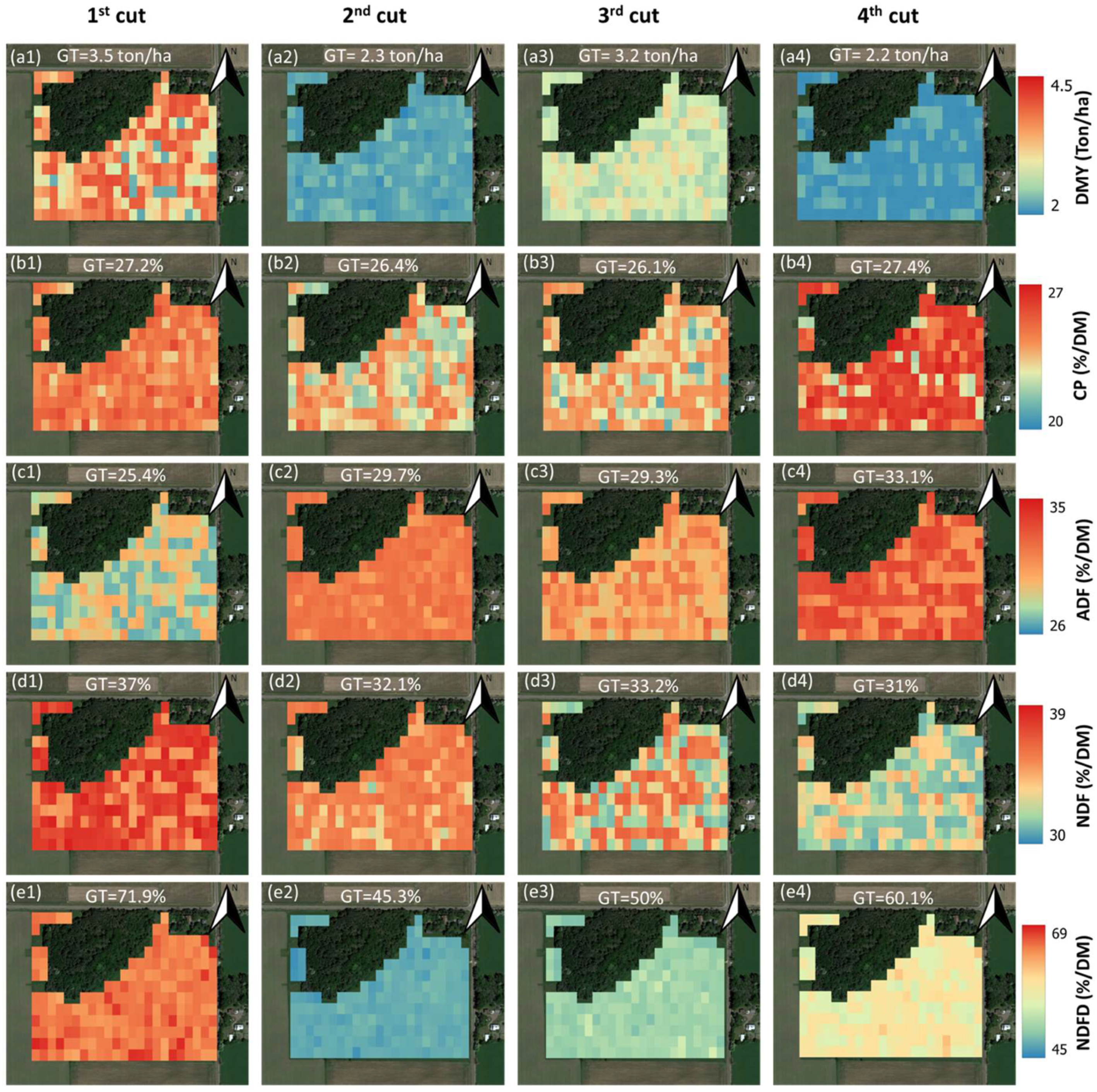
3.5. Visualization of the Estimated Alfalfa DMY and Quality Traits

The estimated maps of an example field are shown in Figure 5 to visualize in-field variations in the alfalfa DMY and quality traits estimated by the XGB model with both environmental factors and SAR features. Each column in Figure 5 shows maps before each cut in the season of 2020. In general, the average values of each map correspond well with their field-level ground data. The estimated maps also demonstrate the spatial variations of each field. Given the complicated interactions of weather, in-field microenvironments, and management activities, alfalfa growth status in fields could be affected as a whole or in specific areas. Using the spatial variation maps, further investigations could be conducted, and decisions could be made regarding field management practices, such as time, amount, and location for precision irrigation, fertilization, and alfalfa cutting windows, so as to maximize production potential, quality, and profitability.

4. Conclusions

The potential to use Sentinel-1 radar features and environmental factors in estimating alfalfa yield and quality was investigated in this study. Radar features and environmental factors, as stably obtainable and low-labor data sources, hold significant applicative value in estimating alfalfa yield and quality, particularly for data that are sparse both temporally and spatially, providing a reference for the long-term stable monitoring of alfalfa. The ANOVA tests show that environmental factors had significant effects on alfalfa traits, and more variations in alfalfa DMY and fiber indicators can be explained when using SAR data. The results from the machine learning modeling show that the Extreme Gradient Boosting model consistently performed the best for all alfalfa traits. The precision of the DMY predictions is deemed acceptable, featuring an average R² of 0.67 and an RMSE of 0.68 tons/ha. For CP content estimation, optimal outcomes were observed with an average R² value of 0.70 and an RMSE of 1.63% DM. In terms of estimating alfalfa’s fiber metrics—namely, ADF, NDF, and NDFD—the best average R² values recorded were 0.54, 0.62, and 0.56, respectively. In our studies, it was observed that solely relying on SAR features for the estimation of alfalfa’s quality traits led to poor performance. The precision achieved through environmental factors markedly surpassed that when using SAR features. Furthermore, when combining the SAR features and environmental factors, the SAR features did not make a noticeable positive contribution to improving the estimation performance. Field maps were generated for alfalfa DMY and quality using the model estimates depicting in-field variations, providing a valuable reference for decision-making related to field management practices and alfalfa harvest time.

References

1. Noland, R.L.; Wells, M.S.; Coulter, J.A.; Tiede, T.; Baker, J.M.; Martinson, K.L.; Sheaffer, C.C. Estimating Alfalfa Yield and Nutritive Value Using Remote Sensing and Air Temperature. Field Crops Res. 2018, 222, 189–196. [Google Scholar] [CrossRef]
2. Radovic, J.; Sokolovic, D.; Markovic, J. Alfalfa-Most Important Perennial Forage Legume in Animal Husbandry. Bio. Anim. Husb. 2009, 25, 465–475. [Google Scholar] [CrossRef]
3. USDA, National Agricultural Statistics Service. Crop Production 2022 Summary; USDA: Washington, DC, USA, 2023.
4. Hancock, D.W.; Collins, M. Forage Preservation Method Influences Alfalfa Nutritive Value and Feeding Characteristics. Crop Sci. 2006, 46, 688–694. [Google Scholar] [CrossRef]
5. Kendall, C.; Leonardi, C.; Hoffman, P.C.; Combs, D.K. Intake and Milk Production of Cows Fed Diets That Differed in Dietary Neutral Detergent Fiber and Neutral Detergent Fiber Digestibility. J. Dairy Sci. 2009, 92, 313–323. [Google Scholar] [CrossRef] [PubMed]
6. Ruppert, L.D.; Drackley, J.K.; Bremmer, D.R.; Clark, J.H. Effects of Tallow in Diets Based on Corn Silage or Alfalfa Silage on Digestion and Nutrient Use by Lactating Dairy Cows1. J. Dairy Sci. 2003, 86, 593–609. [Google Scholar] [CrossRef] [PubMed]
7. Broderick, G.A.; Walgenbach, R.P.; Maignan, S. Production of Lactating Dairy Cows Fed Alfalfa or Red Clover Silage at Equal Dry Matter or Crude Protein Contents in the Diet1. J. Dairy Sci. 2001, 84, 1728–1737. [Google Scholar] [CrossRef] [PubMed]
8. Feng, L.; Zhang, Z.; Ma, Y.; Du, Q.; Williams, P.; Drewry, J.; Luck, B. Alfalfa Yield Prediction Using UAV-Based Hyperspectral Imagery and Ensemble Learning. Remote Sens. 2020, 12, 2028. [Google Scholar] [CrossRef]
9. Feng, L.; Zhang, Z.; Ma, Y.; Sun, Y.; Du, Q.; Williams, P.; Drewry, J.; Luck, B. Multitask Learning of Alfalfa Nutritive Value From UAV-Based Hyperspectral Images. IEEE Geosci. Remote Sens. Lett. 2022, 19, 5506305. [Google Scholar] [CrossRef]
10. Azadbakht, M.; Ashourloo, D.; Aghighi, H.; Homayouni, S.; Shahrabi, H.S.; Matkan, A.; Radiom, S. Alfalfa Yield Estimation Based on Time Series of Landsat 8 and PROBA-V Images: An Investigation of Machine Learning Techniques and Spectral-Temporal Features. Remote Sens. Appl. Soc. Environ. 2022, 25, 100657. [Google Scholar] [CrossRef]
11. Kayad, A.G.; Al-Gaadi, K.A.; Tola, E.; Madugundu, R.; Zeyada, A.M.; Kalaitzidis, C. Assessing the Spatial Variability of Alfalfa Yield Using Satellite Imagery and Ground-Based Data. PLoS ONE 2016, 11, e0157166. [Google Scholar] [CrossRef] [PubMed]
12. Vong, C.N.; Zhou, J.; Tooley, J.A.; Naumann, H.D.; Lory, J.A. Estimating Forage Dry Matter and Nutritive Value Using UAV- and Ground-Based Sensors–A Preliminary Study. In Proceedings of the 2019 ASABE Annual International Meeting, Boston, MA, USA, 7–10 July 2019; American Society of Agricultural and Biological Engineers: St. Joseph, MI, USA, 2019. [Google Scholar]
13. de Castro, A.I.; Shi, Y.; Maja, J.M.; Peña, J.M. UAVs for Vegetation Monitoring: Overview and Recent Scientific Contributions. Remote Sens. 2021, 13, 2139. [Google Scholar] [CrossRef]
14. Maimaitijiang, M.; Sagan, V.; Sidike, P.; Daloye, A.M.; Erkbol, H.; Fritschi, F.B. Crop Monitoring Using Satellite/UAV Data Fusion and Machine Learning. Remote Sens. 2020, 12, 1357. [Google Scholar] [CrossRef]
15. Dvorak, J.S.; Pampolini, L.F.; Jackson, J.J.; Seyyedhasani, H.; Sama, M.P.; Goff, B. Predicting Quality and Yield of Growing Alfalfa from a UAV. Trans. ASABE 2021, 64, 63–72. [Google Scholar] [CrossRef]
16. Chandel, A.K.; Khot, L.R.; Yu, L.-X. Alfalfa (Medicago sativa L.) Crop Vigor and Yield Characterization Using High-Resolution Aerial Multispectral and Thermal Infrared Imaging Technique. Comput. Electron. Agric. 2021, 182, 105999. [Google Scholar] [CrossRef]
17. Shakhatreh, H.; Sawalmeh, A.H.; Al-Fuqaha, A.; Dou, Z.; Almaita, E.; Khalil, I.; Othman, N.S.; Khreishah, A.; Guizani, M. Unmanned Aerial Vehicles (UAVs): A Survey on Civil Applications and Key Research Challenges. IEEE Access 2019, 7, 48572–48634. [Google Scholar] [CrossRef]
18. Colpaert, A. Satellite and UAV Platforms, Remote Sensing for Geographic Information Systems. Sensors 2022, 22, 4564. [Google Scholar] [CrossRef] [PubMed]
19. Bahrami, H.; Homayouni, S.; Safari, A.; Mirzaei, S.; Mahdianpari, M.; Reisi-Gahrouei, O. Deep Learning-Based Estimation of Crop Biophysical Parameters Using Multi-Source and Multi-Temporal Remote Sensing Observations. Agronomy 2021, 11, 1363. [Google Scholar] [CrossRef]
20. Ranjbar, S.; Akhoondzadeh, M.; Brisco, B.; Amani, M.; Hosseini, M. Soil Moisture Change Monitoring from C and L-Band SAR Interferometric Phase Observations. IEEE J. Sel. Top. Appl. Earth Obs. Remote Sens. 2021, 14, 7179–7197. [Google Scholar] [CrossRef]
21. He, M.; Kimball, J.S.; Maneta, M.P.; Maxwell, B.D.; Moreno, A.; Beguería, S.; Wu, X. Regional Crop Gross Primary Productivity and Yield Estimation Using Fused Landsat-MODIS Data. Remote Sens. 2018, 10, 372. [Google Scholar] [CrossRef]
22. Sadenova, M.A.; Beisekenov, N.A.; Apshikur, B.; Khrapov, S.S.; Kapasov, A.K.; Mamysheva, A.M.; Klemeš, J.J. Modelling of Alfalfa Yield Forecasting Based on Earth Remote Sensing (ERS) Data and Remote Sensing Methods. Chem. Eng. Trans. 2022, 94, 697–702. [Google Scholar] [CrossRef]
23. He, M.; Hu, Y.; Chen, N.; Wang, D.; Huang, J.; Stamnes, K. High Cloud Coverage over Melted Areas Dominates the Impact of Clouds on the Albedo Feedback in the Arctic. Sci. Rep. 2019, 9, 9529. [Google Scholar] [CrossRef] [PubMed]
24. Sarafanov, M.; Kazakov, E.; Nikitin, N.O.; Kalyuzhnaya, A.V. A Machine Learning Approach for Remote Sensing Data Gap-Filling with Open-Source Implementation: An Example Regarding Land Surface Temperature, Surface Albedo and NDVI. Remote Sens. 2020, 12, 3865. [Google Scholar] [CrossRef]
25. Ulaby, F.T.; Long, D.G. Microwave Radar and Radiometric Remote Sensing; The University of Michigan Press: Ann Arbor, MI, USA, 2014; ISBN 978-0-472-11935-6. [Google Scholar]
26. Potin, P.; Rosich, B.; Grimont, P.; Miranda, N.; Shurmer, I.; O’Connell, A.; Torres, R.; Krassenburg, M. Sentinel-1 Mission Status. In Proceedings of the EUSAR 2016: 11th European Conference on Synthetic Aperture Radar, Hamburg, Germany, 6–9 June 2016; VDE: Berlin, Germany, 2016; pp. 1–6. [Google Scholar]
27. Crabbe, R.A.; Lamb, D.W.; Edwards, C.; Andersson, K.; Schneider, D. A Preliminary Investigation of the Potential of Sentinel-1 Radar to Estimate Pasture Biomass in a Grazed Pasture Landscape. Remote Sens. 2019, 11, 872. [Google Scholar] [CrossRef]
28. Raab, C.; Riesch, F.; Tonn, B.; Barrett, B.; Meißner, M.; Balkenhol, N.; Isselstein, J. Target-Oriented Habitat and Wildlife Management: Estimating Forage Quantity and Quality of Semi-Natural Grasslands with Sentinel-1 and Sentinel-2 Data. Remote Sens. Ecol. Conserv. 2020, 6, 381–398. [Google Scholar] [CrossRef]
29. Bahrami, H.; Homayouni, S.; McNairn, H.; Hosseini, M.; Mahdianpari, M. Regional Crop Characterization Using Multi-Temporal Optical and Synthetic Aperture Radar Earth Observations Data. Can. J. Remote Sens. 2022, 48, 258–277. [Google Scholar] [CrossRef]
30. Tedesco, D.; Nieto, L.; Hernández, C.; Rybecky, J.F.; Min, D.; Sharda, A.; Hamilton, K.J.; Ciampitti, I.A. Remote Sensing on Alfalfa as an Approach to Optimize Production Outcomes: A Review of Evidence and Directions for Future Assessments. Remote Sens. 2022, 14, 4940. [Google Scholar] [CrossRef]
31. Smeal, D.; Kallsen, C.E.; Sammis, T.W. Alfalfa Yield as Related to Transpiration, Growth Stage and Environment. Irrig. Sci. 1991, 12, 79–86. [Google Scholar] [CrossRef]
32. Suwignyo, B.; Suhartanto, B.; Noviandi, C.T.; Umami, N.; Suseno, N.; Hermanto; Prasetiyono, B.W.H.E. Generative Plant Characteristics Alfalfa (Medicago sativa L.) on Different Levels of Dolomite and Lighting Duration. In Proceedings of the 1st International Conference on Tropical Agriculture, Yogyakarta, Indonesia, 25–26 October 2016; Springer: Berlin/Heidelberg, Germany, 2017; pp. 353–361. [Google Scholar]
33. Ren, L.; Bennett, J.A.; Coulman, B.; Liu, J.; Biligetu, B. Forage Yield Trend of Alfalfa Cultivars in the Canadian Prairies and Its Relation to Environmental Factors and Harvest Management. Grass Forage Sci. 2021, 76, 390–399. [Google Scholar] [CrossRef]
34. Robison, G.D.; Robinson, G.D.; Massengale, M.A. Effect of Night Temperature on Growth and Development of Alfalfa (Medicago sativa L.). J. Ariz. Acad. Sci. 1969, 5, 227–231. [Google Scholar] [CrossRef]
35. Gámez, A.L.; Vatter, T.; Santesteban, L.G.; Araus, J.L.; Aranjuelo, I. Onfield Estimation of Quality Parameters in Alfalfa through Hyperspectral Spectrometer Data. Comput. Electron. Agric. 2024, 216, 108463. [Google Scholar] [CrossRef]
36. Dellar, M.; Topp, C.F.E.; Banos, G.; Wall, E. A Meta-Analysis on the Effects of Climate Change on the Yield and Quality of European Pastures. Agric. Ecosyst. Environ. 2018, 265, 413–420. [Google Scholar] [CrossRef]
37. Andresen, J.A.; Alagarswamy, G.; Rotz, C.A.; Ritchie, J.T.; LeBaron, A.W. Weather Impacts on Maize, Soybean, and Alfalfa Production in the Great Lakes Region, 1895–1996. Agron. J. 2001, 93, 1059–1070. [Google Scholar] [CrossRef]
38. Bertram, M.; Cavadini, J. Wisconsin Alfalfa Yield and Persistence (Wayp) Program 2020 Summary Report; University of Wisconsin-Madison: Madison, WI, USA, 2020. [Google Scholar]
39. Thornton, M.M.; Shrestha, R.; Wei, Y.; Thornton, P.E.; Kao, S.-C.; Wilson, B.E. Daymet: Daily Surface Weather Data on a 1-Km Grid for North America, Version 4 R1; ORNL DAAC: Oak Ridge, TN, USA, 2022. [Google Scholar]
40. Sanderson, M.A.; Karnezos, T.P.; Matches, A.G. Morphological Development of Alfalfa as a Function of Growing Degree Days. J. Prod. Agric. 1994, 7, 239–242. [Google Scholar] [CrossRef]
41. Confalonieri, R.; Bechini, L. A Preliminary Evaluation of the Simulation Model CropSyst for Alfalfa. Eur. J. Agron. 2004, 21, 223–237. [Google Scholar] [CrossRef]
42. dos Santos, E.P.; Da Silva, D.D.; do Amaral, C.H. Vegetation Cover Monitoring in Tropical Regions Using SAR-C Dual-Polarization Index: Seasonal and Spatial Influences. Int. J. Remote Sens. 2021, 42, 7581–7609. [Google Scholar] [CrossRef]
43. Hird, J.N.; DeLancey, E.R.; McDermid, G.J.; Kariyeva, J. Google Earth Engine, Open-Access Satellite Data, and Machine Learning in Support of Large-Area Probabilistic Wetland Mapping. Remote Sens. 2017, 9, 1315. [Google Scholar] [CrossRef]
44. Nasirzadehdizaji, R.; Balik Sanli, F.; Abdikan, S.; Cakir, Z.; Sekertekin, A.; Ustuner, M. Sensitivity Analysis of Multi-Temporal Sentinel-1 SAR Parameters to Crop Height and Canopy Coverage. Appl. Sci. 2019, 9, 655. [Google Scholar] [CrossRef]
45. Lamb, J.F.S.; Sheaffer, C.C.; Rhodes, L.H.; Sulc, R.M.; Undersander, D.J.; Brummer, E.C. Five Decades of Alfalfa Cultivar Improvement: Impact on Forage Yield, Persistence, and Nutritive Value. Crop Sci. 2006, 46, 902–909. [Google Scholar] [CrossRef]
46. Avice, J.C.; Ourry, A.; Lemaire, G.; Volenec, J.J.; Boucaud, J. Root Protein and Vegetative Storage Protein Are Key Organic Nutrients for Alfalfa Shoot Regrowth. Crop Sci. 1997, 37, 1187–1193. [Google Scholar] [CrossRef]
47. Hannaway, D.B.; Shuler, P.E. Nitrogen Fertilization in Alfalfa Production. J. Prod. Agric. 1993, 6, 80–85. [Google Scholar] [CrossRef]
48. Jungers, J.M.; Kaiser, D.E.; Lamb, J.F.S.; Lamb, J.A.; Noland, R.L.; Samac, D.A.; Wells, M.S.; Sheaffer, C.C. Potassium Fertilization Affects Alfalfa Forage Yield, Nutritive Value, Root Traits, and Persistence. Agron. J. 2019, 111, 2843–2852. [Google Scholar] [CrossRef]
49. Laroche, J.-P.; Gervais, R.; Lapierre, H.; Ouellet, D.R.; Tremblay, G.F.; Halde, C.; Boucher, M.-S.; Charbonneau, É. Milk Production and Efficiency of Utilization of Nitrogen, Metabolizable Protein, and Amino Acids Are Affected by Protein and Energy Supplies in Dairy Cows Fed Alfalfa-Based Diets. J. Dairy Sci. 2022, 105, 329–346. [Google Scholar] [CrossRef] [PubMed]
50. Bani, P.; Minuti, A.; Luraschi, O.; Ligabue, M.; Ruozzi, F. Genetic and Environmental Influences on in Vitro Digestibility of Alfalfa. Ital. J. Anim. Sci. 2007, 6, 251–253. [Google Scholar] [CrossRef]
51. Bhattacharya, A. Dry Matter Production, Partitioning, and Seed Yield Under Soil Water Deficit: A Review. In Soil Water Deficit and Physiological Issues in Plants; Bhattacharya, A., Ed.; Springer: Singapore, 2021; pp. 585–702. ISBN 978-981-336-276-5. [Google Scholar]
52. Zhou, H.; Zhou, G.; Song, X.; He, Q. Dynamic Characteristics of Canopy and Vegetation Water Content during an Entire Maize Growing Season in Relation to Spectral-Based Indices. Remote Sens. 2022, 14, 584. [Google Scholar] [CrossRef]
53. Baghdadi, N.; El Hajj, M.; Zribi, M.; Bousbih, S. Calibration of the Water Cloud Model at C-Band for Winter Crop Fields and Grasslands. Remote Sens. 2017, 9, 969. [Google Scholar] [CrossRef]
54. Mandal, D.; Kumar, V.; Lopez-Sanchez, J.M.; Bhattacharya, A.; McNairn, H.; Rao, Y.S. Crop Biophysical Parameter Retrieval from Sentinel-1 SAR Data with a Multi-Target Inversion of Water Cloud Model. Int. J. Remote Sens. 2020, 41, 5503–5524. [Google Scholar] [CrossRef]
55. Graybill, J.S.; Cox, W.J.; Otis, D.J. Yield and Quality of Forage Maize as Influenced by Hybrid, Planting Date, and Plant Density. Agron. J. 1991, 83, 559–564. [Google Scholar] [CrossRef]
56. Phipps, R.H.; Weller, R.F. The Development of Plant Components and Their Effects on the Composition of Fresh and Ensiled Forage Maize: 1. The Accumulation of Dry Matter, Chemical Composition and Nutritive Value of Fresh Maize. J. Agric. Sci. 1979, 92, 471–483. [Google Scholar] [CrossRef]
57. Sanderson, M.A.; Jones, R.M.; Read, J.C.; Lippke, H. Digestibility and Lignocellulose Composition of Forage Corn Morphological Components. J. Prod. Agric. 1995, 8, 169–174. [Google Scholar] [CrossRef]
58. Widdicombe, W.D.; Thelen, K.D. Row Width and Plant Density Effect on Corn Forage Hybrids. Agron. J. 2002, 94, 326–330. [Google Scholar] [CrossRef]
59. Chiu, T.; Sarabandi, K. Electromagnetic Scattering from Short Branching Vegetation. IEEE Trans. Geosci. Remote Sens. 2000, 38, 911–925. [Google Scholar] [CrossRef]
60. Evans, D.L.; Farr, T.G.; van Zyl, J.J.; Zebker, H.A. Radar Polarimetry: Analysis Tools and Applications. IEEE Trans. Geosci. Remote Sens. 1988, 26, 774–789. [Google Scholar] [CrossRef]
61. Patel, P.; Srivastava, H.S.; Panigrahy, S.; Parihar, J.S. Comparative Evaluation of the Sensitivity of Multi-polarized Multi-frequency SAR Backscatter to Plant Density. Int. J. Remote Sens. 2006, 27, 293–305. [Google Scholar] [CrossRef]
Figure 1. Workflow of this study.
Agronomy 14 00859 g001
Figure 2. The two study areas and the distribution of their sampling sites. The RGB images were created using backscattering coefficients derived from Sentinel-1 Ground Range Detected data on 24 July 2020, where blue is σ V V o , green is σ V H o , and red is σ V H o / σ V V o .
Agronomy 14 00859 g002
Figure 3. Boxplots of the alfalfa DMY and quality traits. The cuttings were made at the end of each month from May to August from 2016 to 2021, corresponding to the first to the fourth cuttings. The median value is represented by the line in the middle of the box, and the interquartile range is represented by the box itself. The whiskers extend to the most extreme values that are not considered outliers.
Agronomy 14 00859 g003
Figure 4. Scatterplots of the estimated and measured alfalfa yield and quality traits, with blue dashed lines indicating the ideal condition where predicted data and measured data are the same.
Agronomy 14 00859 g004
Figure 5. Alfalfa yield and quality maps of Sutcliffe field generated using the XGB model. (a1e4) Maps of DMY, CP, ADF, NDF, and NDFD, respectively. GT: ground truth. Background image: Google Earth.
Agronomy 14 00859 g005