Abstract
The microclimate environment can be conveniently controlled with accuracy by plant incubators, in which the cuttings propagation method can efficiently enhance seedling production. To ensure air flow evenly throughout the incubator, the scientific design of the air inlet is crucial. This study utilized a computational fluid dynamics (CFD) model to simulate the airflow patterns in a culture layer under different air inlet conditions. Furthermore, the optimal design parameters were determined by way of response surface methodology (RSM) and the Non-dominated Sorting Genetic Algorithm-II (NSGA-II). Adopting the optimal parameters, a prototype was manufactured, and a cuttings experiment was carried out with apple cuttings in the incubator. The results showed that the optimal air inlet radius is 90 mm, the optimal air inlet height is 188 mm, and the optimal uniform flow plate hole diameter is 13 mm. Meanwhile, the apple cuttings were able to root. Therefore, this incubator with optimal parameters can be used for cuttings. The study provides a methodological and theoretical basis for the future optimizing of air inlet parameters and promoting cuttings rooting.
1. Introduction
Climate change poses continuous threats to plant production and sustainability [1,2]. Evidently, establishing a stable and efficient seedling propagation system is one of the critical challenges for the nursery industry worldwide today [3,4]. Enclosed intensive agricultural buildings have higher efficiency in the utilization of energy, land, water, and carbon dioxide [5].
Gas exchange within a chamber has significant effects on the balance of energy, humidity, and other gases like CO2 and O2 [6,7], which in turn influence plant physiological responses. In an enclosed chamber, a mechanical ventilation system, including fans, ducts, air inlets, and other equipment, is utilized to control airflow to maintain an optimal growing environment. It is indicated in prior studies that promoting air circulation is an important measure for improving crop respiration and photosynthesis [8,9]. However, due to the unique structure of multi-layer or multi-row production areas, the increased resistance to airflow by plants, and the influence of other equipment (such as heat from artificial lights and heating sources), microclimate control in large-scale greenhouses or plant factories becomes more challenging [10]. Therefore, it is necessary to study the airflow in small horticultural facilities. In addition to maintaining even ventilation in the plant canopy, increasing the temperature at the base is beneficial to plant growth. Prior research has analyzed the impact of root temperature on the growth of lettuce [11]; heating the base of cuttings leads to a significant effect on the rooting of woody plant cuttings [12]. Adequate air circulation can maximally control the microclimate environment while minimizing factors that may limit plant growth [13]. Computational fluid dynamics (CFD) is a numerical method that uses finite element analysis to solve fluid flow problems. CFD is a common tool for quantitatively predicting ventilation and thermos fluid physical phenomena [14,15]. Many studies indicate that CFD can predict airflow patterns and ventilation rates inside agricultural buildings based on different building types and chamber dimensions, as well as on the size and location of ventilation openings [13,16,17,18]. With CFD adopted to simulate temperature distributions within chambers [6,19,20], some research has presented comprehensive descriptions of the temperature fields inside the chambers. Heat transfers are influenced by various factors, including air movement, artificial heating (or cooling) sources, plants’ latent and convective exchanges, and the potential heat storage capacity of walls or equipment. For crop cultivation areas, porous medium models based on Darcy’s law have been used to describe the impact of plants on airflow [21]. The influence of various devices in agricultural buildings on the flow field can also be studied through CFD, such as the heat generated by LED light sources and its disturbance to airflow [22,23], as well as the impact of heating devices as energy sources on the airflow distribution within chambers [24,25].
In the design of ventilation systems, the structure of the air inlet is a crucial factor affecting the movement of air inside the environment. Response surface methodology (RSM) can be used to study the relationship between the air inlet structure and airflow [26,27]. RSM, as a tool to find optimal parameter settings, could improve equipment designs by scientists and engineers [28]. RSM can be viewed as a combination of three components, including the design and analysis of experiments, modeling techniques, and optimization methods [29], with each step requiring careful consideration. With regard to interactions among related factors, RSM can generate high-precision predictive models with fewer experiments and is typically used to improve models after identifying significant factors. Prior research has established RSM predictive models based on CFD simulation results to estimate ventilation under different wall openings and ventilation conditions [30,31]. RSM has also been used to simulate the impact of various ventilation forms on indoor environments, reflecting the nonlinear relationship between structural parameters and objectives like airflow velocity and temperature [32]. These studies indicate RSM’s strong potential in researching airflow and ventilation within chambers and establishing corresponding models. In air inlet design, the applicability of the RSM method is worthy of analysis. Classic RSM can be enhanced by modifications to improve the design’s performance. To achieve more accurate models, new methods have been applied in the optimization design field. Studies have used the Non-dominated Sorting Genetic Algorithm-II (NSGA-II) on the basis of RSM to identify optimal design parameter values [33], improving optimization precision and efficiency. As an improvement on the original NSGA, NSGA-II is one of the widely applied multi-objective genetic algorithms (MOGAs), characterized by fast execution speed and better convergence results. Its fast non-dominated sorting mechanism can effectively approximate the Pareto optimal solution [34]. Combining the multi-objective optimization method of RSM with NSGA-II can be applied in the co-optimization of air conditioning systems to find the best parameter settings [35].
Our team has designed the prototype of a cuttings incubator [36]. As part of the project, this study focuses on the design and optimization of air inlets in incubators. To efficiently deliver air at a specified temperature and humidity to the cuttings zone in the incubator during hardwood cuttings propagation, CFD simulations are applied to model the airflow field. With the combination of RSM with NSGA-II, a suitable air inlet structure was designed with the best parameters for the incubator. It was assumed that the actual temperature inside the new prototype would be consistent with the simulation, and the results of the hardwood cuttings propagation will be positive. With its superior environmental control and efficient resource utilization, the incubator can not only enhance propagation efficiency but also expand the scope of plant breeding and agricultural production, which is of application significance for seedling propagation systems.
2. Methods
2.1. Incubator Model Description
Based on existing equipment, this study designed an air inlet structure for a cuttings propagation incubator. Designed for hardwood cuttings, the incubator consists of an environmental controller and the plant incubator (Figure 1). The environmental controller delivers uniformly mixed moist air into the plant incubator body through a ventilation duct, in order to maintain air temperature and humidity within the set limits inside the incubator. To ensure that a single duct provides air with the same temperature and humidity for the three layers of the cultivation zone, an air-guide gap with a width of 80 mm is maintained between the duct and the plant incubator. Equipped with an external insulation layer of 20 mm, the plant incubator has dimensions of 1260 mm × 810 mm × 1900 mm, ensuring better thermal insulation performance. The ventilation duct and air-guide gap are also insulated. The incubator features a forced ventilation system, while the top three layers serve as plant cultivation layers, each with a height of 540 mm. With a height of 280 mm, the lowest layer is used for collecting waste liquid. Under the Polyvinyl Chloride (PVC) seedling trays holding the substrate, there are thermostatic plates to maintain the substrate temperature.
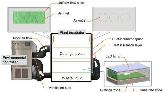
Figure 1.
Environmental control system diagram of cuttings. The white arrow shows the direction of moist airflow: from the left side of the environmental controller through the vent into the plant incubator, the duct-incubator space acts as a buffer so that the moist air can be evenly distributed in the three culture layers, and then returned to the environmental controller from the right side (the return pipe runs around the back of the incubator). Each cuttings layer consists of a lamp zone, a cuttings zone, and a substrate zone. The inlet and outlet are on opposite sides, and the inlet is equipped with an even-flow plate.
It is assumed that each layer of the plant cultivation layers in the incubator is independent. The light zone is set at a 40 mm height and 650 mm width, while the substrate zone is set at a 100 mm height and 650 mm width. The cuttings zone is 1070 mm in length and 550 mm in width. The height of the above-ground part of the cuttings is presumed to be 60 mm. The sides of the plant incubator are respectively equipped with air inlet and an outlet. The environmental controller mixes air with water vapor evenly, which is then introduced from the inlet on the left side into the incubator through the forced ventilation system. The returning airflow exits the plant incubator through the outlet on the right side. A partial model of plants was constructed, focusing only on the light area and substrate area, while support frames, connecting devices, and other similar structures are disregarded in the model.
2.2. CFD Model
2.2.1. Governing Equation
The fundamental control equations in CFD numerical simulations include the continuity equation, the momentum equation, and the energy equation [37].
The continuity equation is as follows:
where t represents time in seconds (s); xi is the coordinate in the i direction (m); and υi is the velocity component in the i direction (m s−1).
The momentum equation is as follows:
where δij represents the components of the stress tensor (kg s−1 m−2); gi is the component of gravitational acceleration in the i direction (m s−2); μ′i is the fluctuating velocity component in the i direction (m s−1); and μ′j is the fluctuating velocity component in the j direction (m s−1).
The energy equation is as follows:
where Cp represents the specific heat capacity of air (J kg−1 K−1); T denotes the air temperature (K); λf is the thermal conductivity of air (W m−1 K−1); μt indicates the turbulent viscosity of air (kg s−1 m−2); and Pt stands for the turbulence Prandtl number.
Considering that the airflow within the plant incubator exhibits significant turbulent characteristics, this study employs the standard k-ε turbulence model, known for its excellent convergence and high computational precision, to solve the airflow dynamics inside the incubator [38,39].
2.2.2. Thermostatic Plate and Substrate
In this study, temperature control of the substrate was achieved using a thermostatic plate based on water circulation control (Figure 2). Four PVC trays filled with a mixed substrate were placed on the thermostatic plate. The composition and moisture content of the substrate significantly influence its thermal properties, which in turn affect the heat exchange among the thermostatic plate, substrate, and air. The thermophysical properties of the substrate can either be determined by experimental measurements or calculated by empirical formulas. The substrate in this research is made up of a mixture of perlite, vermiculite, and peat. The substrate’s bulk density and volumetric water content were measured, and then its thermal conductivity and specific heat capacity were calculated with the effective conductivity model [40,41].
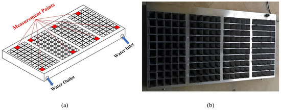
Figure 2.
Thermostatic plate for controlling substrate temperature. (a) Diagram of measurement points, featuring partitions in the thermostatic plate to ensure uniform water flow; (b) Real thermostatic product.
In order to validate the heat conduction between the thermostatic plate, substrate, and air, a prototype of the thermostatic plate was constructed, which operated under a constant environmental temperature of 21 °C. An environmental controller provided circulating water for the thermostatic plate, maintaining the inlet water temperature at 24 °C. Closed-loop feedback regulation was employed. The measurement points are illustrated in Figure 2a. A four-channel thermocouple thermometer (model: TA612C, Suzhou Tasi Electronic Industrial Co., Ltd., Suzhou, China) was utilized to measure the surface temperature of the thermostatic plate, which recorded the time of temperature stability. Once a stable temperature was attained, the Uniformity Index (UI) was calculated according to Equation (4) [23]:
where is the number of measurement points; Ti is the temperature at the ith measurement point (°C); and represents the average temperature of all the measurement points (°C).
PVC trays filled with substrate were placed on the thermostatic plate for closed-loop feedback regulation. The substrate temperature was measured at a depth of 5 cm. Meanwhile, the time for temperature stabilization was recorded. After stabilization, the Uniformity Index (UI) of the substrate temperature was calculated. A CFD model was developed for the experimental setup under the same operating conditions. The reliability of the model was validated by comparing the simulated values with the measured values.
2.2.3. LED Lamp
The light source inside the incubator is LED, whose heat flux q is calculated in accordance with the electrical efficiency [42] and Equation (5). In each cultivation layer, there are four LED tubes (rated 24 W, model: 5B24C-120LED, HiPoint Inc., Gaoxiong, Taiwan, China). Each tube contains 120 LED beads.
where E is the electrical input power (W); η is the electrical efficiency; VLED is the volume of LED beads (m3); and nl is the number of LED beads.
To validate the energy source of the LED lamps and the heat exchange between the LED lamps and air, it is necessary to measure the surface temperature of the lamp under a constant ambient temperature of the stable temperature of 21 °C, calculating the temperature UI. A CFD model was established, operating under the same environmental conditions. By comparing the simulated values with the measured values, the reliability of the LED lamp model can be verified.
2.2.4. Porous Media
Cuttings can create certain obstructions to airflow, resulting in a loss of momentum as well as ventilation problems. In this study, a porous medium model is adopted as it describes the physical characteristics of air movement above the cuttings. When steady, low-speed, incompressible air passes through a porous medium, the resulting momentum source term (Si) can be expressed by the Darcy–Forcheimer equation [43]:
where μ is the air dynamic viscosity (kg s−1 m−1); ρ is the air density (kg m−3); K is the permeability of the porous medium (m2); υ is the wind speed (m s−1); Cf is the nonlinear momentum loss coefficient (m−1); C1 is the viscous resistance factor (m−2); and C2 is the inertial resistance factor (m−1).
The magnitude of K could be calculated by using Kozeny’s equation [44]:
where dp is the average leaf length (m) and ϕ is the porosity of the porous medium. The values of dp = 0.05 m and ϕ = 0.97 were measured and adopted in this study.
The loss of momentum caused by the crop’s drag effect can be quantified using the measurement of a unit of volume of the canopy cover [39], which can obtain:
where L is the leaf area density (m−2 m−3) and Cd is the drag coefficient. Research has conducted experiments and determined the drag coefficients for four types of crops, namely, tomato, sweet pepper, eggplant, and soybean, which are 0.26, 0.23, 0.23, and 0.22, respectively [45]. At certain wind speeds, the differences in drag coefficients among these four crops are not significant. In this study, the drag coefficient was set at 0.22.
2.2.5. Respiratory Heat
By way of respiration during their normal physiological activities, cuttings will generate CO2 and energy. An equation representing respiration with glucose as the substrate is established as shown in Equation (11) [46]:
In a sealed system, the respiration rate of the cuttings is measured. The calculation of the respiration rate is as shown in Equation (12) [47]:
where is the respiratory rate (g m−3 h−1); ∆t is the time interval between two measurements (h); and is the difference in carbon dioxide concentration between two measurements.
For every 1 mole of glucose consumed, 6 moles of CO2 are produced, while releasing 2816 kJ of heat energy [46]. The respiratory heat is calculated by Equation (13):
where Q is the respiratory heat (kJ h−1) and α is the heat loss rate. During the process of respiration, 60% of the energy is released in the form of heat. Vc is the volume of cuttings in the sealing system (m3) and is the molar mass of CO2, equal to 44 g mol−1. Based on the respiratory heat obtained in the sealed system, the heat flux of all the cuttings inside the incubator can be calculated by Equation (14):
where q is the heat flux (W m−3) and Vt is the total volume of cuttings in the incubator (m3).
2.3. Boundary Conditions
The air inside the incubator is considered a homogeneously incompressible gas, flowing at low speed in a normal temperature environment. The airflow in the incubator conforms to the Boussinesq approximation, with the presence of natural convection and isothermal forced flow, taking into account the effect of buoyancy due to the effect of temperature changes on air movement.
The materials used in the CFD model include an air mixture composed of air and water vapor, as well as solid materials such as substrate, glass, and cuttings. The physical properties of these materials are shown in Table 1. The relevant physical parameters for air, glass, plastic, and aluminum are referenced from the study by Zhang et al. [48]. The boundary conditions are set as shown in Table 2. The boundary inlet is defined as a velocity inlet, with a wind speed of 1.5 m/s, a temperature of 21 °C, and a relative humidity of 85%. The boundary outlet is defined as a pressure outlet. The incubator body is wrapped in insulating material on all sides. In addition, the heat exchange with the outside air can be approximately neglected. Heat transfer through thin shells is set between the light area and the air, the substrate area and the air, and the substrate area and the plants.

Table 1.
Physical properties of materials.
Table 2.
Boundary conditions of CFD simulations for air inlet design and ventilation.
2.4. Grid Quality and Solver Settings
Based on the geometric model, hexahedral and tetrahedral elements were used to create the grids. The air and plants inside the incubator were treated as fluid computational domains, while the light area and substrate were considered as solid computational domains. In the plant area and incubator air part, the maximum cell length is 3 mm, forming an unstructured grid. Local grid refinement was applied to the inlet, outlet, and crop areas to capture the flow characteristics in these crucial regions. The mesh has a minimum Orthogonal Quality of 0.2 and passed mesh quality checks and smoothing processes, confirming its effectiveness.
The air inside the plant incubator can be considered a mixture of dry air and water vapor. It had been assumed to be an incompressible Newtonian fluid, while the water vapor did not undergo phase change. A mixed mathematical model has been used for analysis of the multiphase gas flow field. The wall function approach was employed for the near-wall regions. The component transport model described the convective diffusion process of the humid air inside the incubator and the external environment. Based on Darcy’s law, a porous medium model was established between the crop layer and the internal airflow velocity. The SIMPLEC algorithm was used for discretization and pressure–velocity coupling. For spatial discretization, the diffusive terms of all the equations were solved by way of the least squares method. Standard interpolation was used to calculate the pressure on the cell faces, thereby computing pressure gradients. Discretization schemes were used for the pressure. For the convection terms of momentum, continuity, and energy, the second-order upwind interpolation scheme was employed. For the turbulent kinetic energy and turbulent dissipation rate, the first-order upwind discretization schemes were used for better convergence in computations. The convergence criteria for the continuity, momentum, and energy terms were set at 10−6, while for the viscous terms they were set at 10−3. Solution convergence was confirmed by monitoring the residuals.
2.5. Parameter Optimization
Because of the constraints of the plant incubator (Figure 1) structure, the optimization variables were defined as the radius of the air inlet (Ra), the height of the air inlet (Ha), and the diameter of the holes in the even-flow plate (Dp). The value ranges for each parameter were determined based on the results of the single-factor analysis and will be described in Section 3.2.1. To further enhance the performance of the incubator, the study sought the best air inlet design parameters based on the regression equation obtained, which will provide the optimal growth environment for cuttings. The method of evaluating the growth environment for cuttings is as crucial as the choice of objective functions. The interplay between and constraints imposed by the wind speed, temperature, and humidity form a complex coupled physical field within the incubator, which make it inevitable for multi-objective functions to be used to evaluate the thermal environment of the incubator. Cuttings need a full-humidity environment for rooting, while too low a wind speed can result in water vapor condensation and cause rotting. Moreover, in the long-term enclosed environment of an incubator without ventilation, the ratio of carbon dioxide and oxygen is hard to balance, and harmful gases could accumulate, which could damage the cuttings. Additionally, heating the base of the cuttings while maintaining a certain temperature difference with the top can facilitate the production of more roots. Therefore, two objective functions were selected, that is, wind speed (vs) and temperature difference (∆T), serving as a comprehensive evaluation of the environment inside the incubator, which is defined as follows:
Constraints are the various limitations imposed on decision-making solutions when addressing planning problems. Based on the structural limitations of the incubator, the constraints for the relevant structural parameters are proposed as follows:
To verify the practical effectiveness of the inlet design, the hardwood cuttings experiments were conducted using a prototype. The experiments were conducted in the Agricultural Equipment Informatization and Intelligence Laboratory of the Hebei Smart Agriculture Equipment Technology Innovation Center. Through the analysis of the temperature measurements and cuttings experiment results, the reliability of the optimized results from the CFD simulation was verified. The environmental controller and the plant incubator were placed in a laboratory where the air temperature could be adjusted to minimize external environmental interference. The environmental controller was used to control the conditions inside the incubator, setting the air temperature at 21.0 °C, relative humidity at 85%, and substrate temperature at 24.0 °C. The temperatures at the top of the cuttings, the base of the cuttings (i.e., 5 cm deep in the substrate), and the surface of the substrate were measured. The measurement points are shown in Figure 2a, and the measurements were taken with the incubator door closed.
3. Results
3.1. Model Validation
The time was measured from when the circulating water entered through the inlet of the thermostatic plate. After 5 min, the temperature at the measurement points on the surface of the thermostatic plate stopped rising, enabling a comparison between the simulated and experimental measured values (Figure 3a). The average temperatures of the thermostatic plate surface, as simulated and measured, were 24.0 °C and 24.3 °C, respectively. The temperature distribution simulated by the CFD model was much more even compared to the actual measurements, with a simulated UI of 0.9925 and a measured UI of 0.9771.
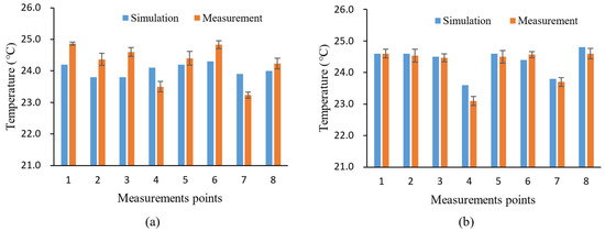
Figure 3.
Thermostatic plate and substrate model validation. (a) The simulated and experimental measured temperature of the thermostatic plate surface without substrate; (b) The simulated and experimental measured temperature of the substrate (5 cm depth) with substrate. The error line represents the standard deviation of multiple readings at the measurement points.
After draining the water from the thermostatic plate, the PVC trays filled with substrate were placed in position, and the thermometer probe was positioned at a depth of 5 cm at the measurement point. After 12 min, the temperature at the measurement point remained constant. The simulated and actual measured values were compared (Figure 3b). The average temperatures of the thermostatic plate surface, as simulated and measured, were 24.4 °C and 24.3 °C, respectively. The UI simulated by the CFD model was 0.9836, which was much more even compared to the actual measured UI of 0.9789.
The surface temperature of the simulated LED lamp was compared with the corresponding points measured in the experiment (Figure 4). The average difference between simulated and measured temperatures was 0.6 °C, and the UI of the two were 0.9863 and 0.9769, respectively. The accuracy of the model in predicting the surface temperature of the LED lamp was slightly lower than that of the surface temperature of the thermostatic plate and the substrate temperature, with an error of less than 10%, which is considered acceptable.
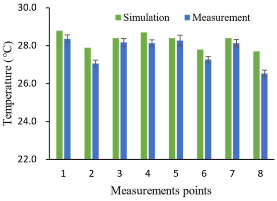
Figure 4.
LED lamp model validation. The 8 points of measurement are distributed equidistantly on an LED lamp. The error line represents the standard deviation of multiple readings at each measurement point.
This study assumed that the heat dissipation of the LED lamps was even. In fact, due to the instability of the air conditioning in the room, the air temperature was constantly changing. Therefore, inaccurate environmental conditions may have led to inaccurate temperature predictions. However, the thermostat was adjusted in real-time by the controller to ensure that the actual situation was more consistent with the simulated situation. In particular, the temperature of the thermostatic plate was regulated by circulating water, and the higher specific heat capacity of water can maintain the strong thermal inertia and consistency of the thermostatic plate.
3.2. Design of Air Inlet
3.2.1. Single-Factor Numerical Fitting
The number of air inlets, Ra, and Ha are factors that affect the flow field and temperature inside the incubator, because the cuttings incubator needs ventilation to maintain the aeration of the cuttings canopy, and reduce the influence of LED lamp heat dissipation. Meanwhile, the airflow should not be too strong, in order to maintain the temperature difference between the upper and lower parts of the cuttings. Different levels for these factors were set (Table 3) and single-factor simulation experiments were conducted (the parameters for the air inlets on both sides were set the same). The results of the 1st to 3rd group of simulation experiments are shown in Figure 5 (at 165 mm high plane). As the number of air inlets increased, the wind speed in the cultivation layer became more even, with the air inlet number at 3 showing a relatively more even wind speed. To further improve the uniformity of the wind speed, an even-flow plate was added at the left air inlet. The diameter of the small holes in the even-flow plate also affected the flow field inside the incubator. The impact of the diameter of the even-flow plate holes on the flow field was analyzed through experiments in groups 18 to 24.
Table 3.
Single-factor experiment table.
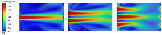
Figure 5.
Simulation experiment results for the number of air inlets.
After conducting simulations through Fluent 19.0, the wind speed at the surface of the cuttings canopy (vs) and the temperature difference between the upper and lower parts of the cuttings (∆T) under different air inlet parameters were obtained. As shown in Figure 6, as Ra increased, vs gradually rose; simultaneously, there was a significant increase in the Ra interval of [70, 100]. The temperature difference showed a trend of rising at first, followed by falling, before reaching a maximum value when Ra was 80.
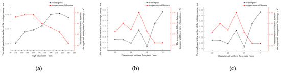
Figure 6.
Influence of different structural parameters on airflow based on single-factor parameter analysis. (a) Radius of air inlet (Ra); (b) Height of air inlet (Ha); (c) Diameter of even-flow plate (Dp).
Along with the increase in Ha, both vs and ∆T showed a trend of initially increasing and then decreasing, while vs reached a maximum value if Ha reached 200. ∆T reached its maximum when Ha was 170. When Dp ranged from 13 to 17, vs exhibited significant fluctuations, reaching a minimum when Dp was 16. When Dp ranged from 12 to 16, ∆T showed significant fluctuations, reaching a maximum when Dp reached 15.
3.2.2. Orthogonal Experiment and Multivariate Model Establishment
Based on the results of the single-factor experiment analysis, a reasonable range of structural parameters was selected. A three-factor three-level experimental table was designed, as shown in Table 4, to conduct response surface experiments. These experiments explored the interactions among the three factors to determine the optimal parameter combination. The average wind speed at the surface of the cuttings canopy was chosen as the response value Y1, and the temperature difference between the upper and lower parts of the cuttings as the response value Y2. The analysis was conducted using the Design-Expert 13.0 software, and the results of the model variance analysis are shown in Table 5.
Table 4.
Factor level.
Table 5.
Significance and analysis of variance.
The significance and variance analysis of Y1 in Table 5 evidenced that the model term was highly significant (p < 0.0001), while the lack-of-fit was not significant (p = 0.0504). This indicated that the model was significantly valid, with no lack-of-fit factors present and minimal error. A high degree of model fitting was suggested (R2 = 0.9682). For the influence on Y1, A, AB, AC, BC, A2, and C2 were highly significant. The order of influence of each factor was A > B > C. The regression equation is as follows:
Similarly, the model for Y2 was significantly valid, with no lack-of-fit factors present and minimal error (the model term was highly significant (p = 0.0001) and the lack-of-fit was not significant (p = 0.1204)). The fit statistic R2 was 0.9781, suggesting a high degree of model fitting. For the influence on Y2, A, B, AB, A2, and C2 were highly significant. The order of influence of each factor was B > A > C. The regression equation is as follows:
The influence of significant interaction factors on the response values is shown in Figure 7. As can be observed from Figure 7a, when A is constant, Y1 initially increases and then decreases along with an increase in B; and when B is constant, Y1 decreases first and then increases with an increase in A. As shown in Figure 7b, when A is constant, Y1 increases with an increase in C; and when C is constant, Y1 gradually increases with an increase in A. As shown in Figure 7c, when B is constant, Y1 slowly decreases; and when C is constant, Y1 initially increases and then slowly decreases with an increase in B. Finally, as shown in Figure 7d, when B is constant, Y2 initially decreases and then increases with an increase in C; and when C is constant, Y2 increases with an increase in B.
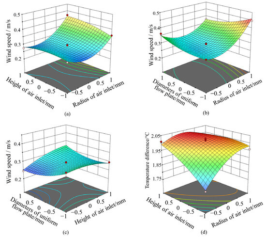
Figure 7.
Response surface indicating the influence of interaction factors on response value. (a–c) Interaction effect of AB, AC, BC on Y1; (d) interaction effect of AB on Y2.
3.3. Optimization of Air Inlet
3.3.1. Optimization Results
In the study, NSGA-II is used for optimization, with a population of 50 individuals in each generation. The algorithm selects the best individuals from the parent population and directly transfers them to the offspring population. The remaining individuals in the offspring population are generated through crossover and mutation between the parent individuals. The final Pareto optimal solution set is obtained by considering constraint conditions and convergence criteria. Multi-objective genetic algorithms have a high convergence efficiency and can quickly search for the optimal results.
After 200 iterations, a total of 70 feasible design solutions that met the constraint conditions were generated. Figure 8 shows the distribution of the optimization results, with the horizontal axis representing the values of the objective function f1 for each solution and the vertical axis representing the values of the objective function f2. It can be observed that the optimal design solutions located on the Pareto front are marked with red squares. The parameters of the four optimal solutions were rounded to determine the optimal designs as follows: air inlet radius of 90 mm, air inlet height of 188 mm, and even-flow plate hole diameter of 13 mm.
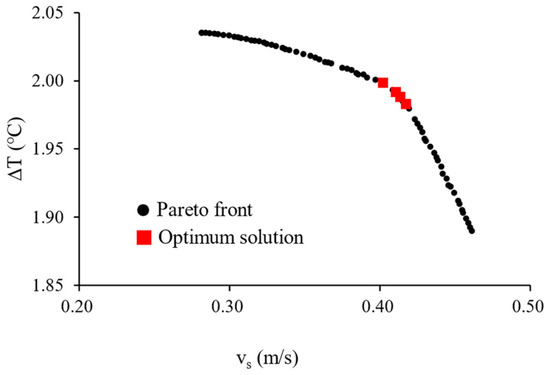
Figure 8.
Pareto front and optimization results.
3.3.2. Parameter Validation
The temperature and airflow velocity distribution for the optimal design results were validated through experimental testing. A CFD model was established with the optimal design parameters, and Figure 9 shows the temperature and airflow velocity distribution for a culture layer in the incubator corresponding to the optimal inlet design. From the figure description, it can be observed that the airflow velocity distribution at the top of the cuttings was relatively even, and the temperature difference between the upper and lower parts of the cuttings was greater than 3 °C, which meets the requirements of rooting.
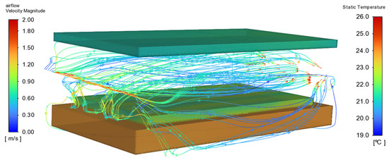
Figure 9.
The temperature and wind speed distribution of the optimal design results. The streamline indicates the flow pattern within the cuttings layer, and its color indicates the air velocity magnitude; the colors of the LED lamp, cuttings zone, and substrate zone indicate the temperature contours.
The actual temperature measurements during the propagation are shown in Table 6; the model’s accuracy was verified by way of the Mean Relative Error (MRE) and Root Mean Square Error (RMSE). The actual temperatures at the top of the cuttings, the base of the cuttings, and the substrate surface showed minimal deviation from the simulated values, and the UI of the actual values was >0.98, indicating a relatively even temperature distribution within the incubator. The air temperature was set at 21 °C and the substrate temperature was set at 24 °C. The average temperatures at the base of the cuttings, 5 cm deep in the substrate, were 24.0 °C and 24.2 °C, respectively. The average temperatures of the substrate surface were 23.0 °C and 23.1 °C, respectively. The temperature of the substrate surface is lower than that of the substrate 5 cm deep because the ventilation reduces the heat of the substrate surface, while the thermostatic plate heats the substrate continuously, and the thermal conductivity of the substrate is small, so heat can be retained. The average temperatures at the top of the cuttings were 21.1 °C and 21.2 °C, respectively, both slightly higher than the set values. This shows that the heat dissipation effect of various devices cannot be completely offset by ventilation. However, the observed experimental results showed the temperature difference between the upper and lower parts of the cuttings were still maintained at 3 °C, and met the needs of the cuttings’ roots.
Table 6.
Actual temperature measurement results of the cuttings experiment.
Apple (Malus pumila) branches were collected for the cuttings on 9 April 2023, using the SH-40 variety (Figure 10a). Six days after cultivation, the cuttings began to sprout (Figure 10c). Twelve days later, a large amount of callus tissue appeared. By the 18th day, significant root systems emerged (Figure 10b). The cuttings experiment demonstrated that the air inlet designed in this study could ensure even temperature distribution within the incubator. Despite the condition of heat generated by the thermostatic plate, LED lighting, and cuttings respiration, a constant temperature difference was kept between the upper and lower parts of the cuttings. In the relatively enclosed environment of the incubator, the conditions necessary for rooting hardwood cuttings were satisfactorily met.
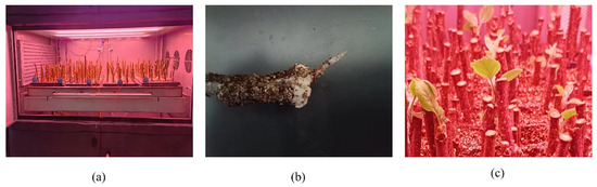
Figure 10.
Cuttings and rooting experiment. (a) Cuttings experiment site; (b) Rooting of cuttings; (c) Sprouting of cuttings.
4. Discussion
With the development of the nursery industry, more and more research is focusing on the growth conditions of seedlings in controlled environments, including how to provide an appropriate growing environment for cuttings propagation [49,50,51]. To study plant growth in microclimatic environments, CFD models have been established. Some studies focus on the interaction between environmental factors like temperature, humidity, and CO2, utilizing air conditioning and fans to improve airflow distribution and reduce environmental variability [52,53]. In these CFD models, some research concerns the exchange of airflow inside and outside the facility as well as the impact of solar radiation [19], some research takes crops as a unified entity and incorporates them as porous media in simulation calculations [22], and some research involves the effect of LED light heat dissipation on airflow [54]. However, these studies predominantly focus on greenhouses or plant factories, whereas this study involves cuttings in an artificially controlled incubator, where airflow is more sensitive to various factors in a relatively confined space. Consequently, in addition to the heat dissipation of the thermostatic plate and LED lights, this study also considers the respiratory heat produced by the life activities of the cuttings. Unlike our study, all the research mentioned above did not consider the heat dissipation of plants to the environment, but considered only the impact of the external environment or equipment on the plants in the CFD model.
A substrate temperature higher than the air temperature can promote the growth process of plants [55]. Compared with non-heating of the substrate, heating the base of cuttings under low-temperature conditions is beneficial for rooting and subsequent growth [56]. Moreover, increasing the temperature at the base of the cuttings while maintaining the same air temperature can increase root mass and plant height, which has been confirmed in many herbaceous plants [57,58], and is even more effective for woody plant cuttings [12]. For most woody plants, cuttings propagation is typically carried out with air temperatures set between 18 and 24 °C, and substrate temperatures maintained between 20 and 25 °C through heating [59]. In this study, these air temperature settings were considered in the validation of apple hardwood cuttings. Accordingly, this study used a thermostatic plate to heat the base of the cuttings to promote rooting, providing continuous ventilation to ensure a certain temperature difference between the upper and lower parts of the cuttings. In greenhouses, studies have used electric heating wires and plates to heat the substrate [60], and many have used rubber tubes or steam pipes to provide the heat [61,62,63]. Heating wires, tubes, or pipes heat the substrate unevenly; heating plates are better, but they can transfer heat from only one side. As Figure 2 shows, our thermostatic plate can transfer heat from multiple sides, and the problem of uneven heating has been improved. The heat provided via heating equipment to the substrate in greenhouses can spread naturally, but that is not at all the case in the incubator. Due to the small height of the cuttings and the cultivation space being much smaller than the greenhouse, a forced ventilation system through the controller was added to provide humid air for the canopy layer of the cuttings, aiming at ensuring a temperature difference between the top and base of the cuttings while providing appropriate humidity for rooting.
The position and structure of the air inlet have a significant impact on ventilation. Research comparing five different ventilation layouts in plant factories has analyzed the uniformity of microclimates under different ventilation conditions [39]. This study used RSM to establish a model, and NSGA-II was adopted to determine the optimal air inlet structure design quantitatively. Moreover, the corresponding correlation coefficients (R2) of 0.9682 and 0.9781 indicated high model fidelity and reliability. The airflow enters from the left inlet without resistance and moves rapidly to the right under the action of the fan, exiting through the right outlet, which makes it difficult for the air to flow around and downward, leading to reduced convective heat transfer and uneven temperature distribution in the space. Therefore, it is necessary for researchers to add an even-flow plate to improve the uniformity of environmental factors within the plant factory [64]. However, their study used only a full mesh ventilation wall of a single size to discuss its effect on reducing local environmental differences, whereas this study obtained a more suitable aperture size for the even-flow plate through RSM and NSGA-II.
The temperature distribution is greatly influenced by airflow patterns. Since the airflow inside the incubator is characterized by high turbulence, representing a highly complex nonlinear movement, and the subject of this study is hardwood cuttings with a relatively small leaf area, employing resistance coefficients from other studies in simulations might increase the error between the simulation results and actual values. In addition, we focus on hardwood or semi-hardwood cuttings and do not give much consideration to herbage in the process of CFD modeling. Meanwhile, cuttings require humidity control, which is achieved in greenhouses through intermittent misting to control the vapor pressure deficit (VPD) [65]. VPD is a key regulator of transpiration [66]; various studies have discussed the interaction of VPD, transpiration, and airflow in chamber CFD modeling [10,23,39]. In conclusion, the flow field simulation of the incubator can be further optimized to adapt to cuttings from multiple types of plants in future studies.
5. Conclusions
In order to improve the uniformity of the flow field inside the incubator, the air inlet needs to be designed and optimized. Using CFD for numerical simulation analysis, the evenness of the airflow field under different structural parameters of the culture layer air inlet is compared. Through single-factor experiments, the ranges of the structural parameters were determined. Within a reasonable range, a response surface model between the structural parameters and response values was established through orthogonal experiments. On this basis, using the NSGA-II algorithm, the optimal design parameters were determined. The optimal design parameters were determined to be as follows: an air inlet radius of 90 mm, an air inlet height of 188 mm, and an even-flow plate hole diameter of 13 mm. Under these optimal parameters for the culture layer air inlet structure, experimental validation was conducted. The rooting of the apple hardwood cuttings confirmed the effectiveness of the ventilation system, proving that as a kind of vertical facility, the incubator is feasible for cuttings. Seedling cultivation through cuttings in vertical facilities could save resources, expand planting scope, and contribute to the development of the future seedling industry.
Author Contributions
H.G. designed the experiments, collected the data, analyzed the statistics, and wrote and revised the manuscript. J.Q. designed the experiments and wrote and revised the manuscript. S.L. collected the data and analyzed the statistics. J.L., X.W. and Z.J. were responsible for the verification of the results. X.Y. designed the experiments, proposed the work, was the main supervisor and advisor, and revised the manuscript. All authors have read and agreed to the published version of the manuscript.
Funding
This work was supported by the earmarked fund for the China Agriculture Research System (CARS-27) and Hebei Agriculture Research System (HBCT2024200404).
Data Availability Statement
All the data generated or analyzed during this study are included in this published article.
Acknowledgments
We appreciate Hi Point Inc. (Gaoxiong, Taiwan, China) for providing technical support.
Conflicts of Interest
The authors declare no conflicts of interest.
References
- Anderson, J.T.; Song, B. Plant Adaptation to Climate Change—Where Are We? J. Syst. Evol. 2020, 58, 533–545. [Google Scholar] [CrossRef]
- Wheeler, T.; Von Braun, J. Climate Change Impacts on Global Food Security. Science 2013, 341, 508–513. [Google Scholar] [CrossRef]
- Singh, D.; Kumar, A. Multivariate Screening Approach Indicated Adaptive Tolerance to Salt Stress in the Seedlings of an Agroforestry Tree, Eucalyptus Tereticornis Sm. Plant Cell Tiss. Org. 2021, 145, 545–560. [Google Scholar] [CrossRef]
- Wang, H.; Zhou, Z.; Yang, Z.; Cao, Y.; Zhang, C.; Cheng, C.; Zhou, Z.; Wang, F.; Hu, C.; Feng, X.; et al. Constraints on the high-quality development of Chinese fruit industry. China Fruits 2023. [Google Scholar] [CrossRef]
- Graamans, L.; Baeza, E.; Van Den Dobbelsteen, A.; Tsafaras, I.; Stanghellini, C. Plant Factories versus Greenhouses: Comparison of Resource Use Efficiency. Agric. Syst. 2018, 160, 31–43. [Google Scholar] [CrossRef]
- Bartzanas, T.; Boulard, T.; Kittas, C. Effect of Vent Arrangement on Windward Ventilation of a Tunnel Greenhouse. Biosyst. Eng. 2004, 88, 479–490. [Google Scholar] [CrossRef]
- Lee, I.-B.; Short, T.H. Two-Dimensional Numerical Simulation of Nutaral Ventilation in a MultI-Span Greenhouse. Trans. ASAE 2000, 43, 745–753. [Google Scholar] [CrossRef]
- Kitaya, Y.; Tsuruyama, J.; Shibuya, T.; Yoshida, M.; Kiyota, M. Effects of Air Current Speed on Gas Exchange in Plant Leaves and Plant Canopies. Adv. Space Res. 2003, 31, 177–182. [Google Scholar] [CrossRef]
- Roy, J.C.; Pouillard, J.B.; Boulard, T.; Fatnassi, H.; Grisey, A. Experimental and CFD Results on the CO2 Distribution in a Semi Closed Greenhouse. Acta Hortic. 2014, 1037, 993–1000. [Google Scholar] [CrossRef]
- Tamimi, E.; Kacira, M. Analysis of Climate Uniformity in a Naturally Ventilated Greenhouse Equipped with High Pressure Fogging System Using Computational Fluid Dynamics. Acta Hortic. 2013, 1008, 177–183. [Google Scholar] [CrossRef]
- Carotti, L.; Graamans, L.; Puksic, F.; Butturini, M.; Meinen, E.; Heuvelink, E.; Stanghellini, C. Plant Factories Are Heating Up: Hunting for the Best Combination of Light Intensity, Air Temperature and Root-Zone Temperature in Lettuce Production. Front. Plant Sci. 2021, 11, 592171. [Google Scholar] [CrossRef]
- Confalonieri, M.; Balestrazzi, A.; Bisoffi, S.; Carbonera, D. In Vitro Culture and Genetic Engineering of Populus Spp.: Synergy for Forest Tree Improvement. Plant Cell Tiss. Org. 2003, 72, 109–138. [Google Scholar] [CrossRef]
- Bournet, P.-E.; Boulard, T. Effect of Ventilator Configuration on the Distributed Climate of Greenhouses: A Review of Experimental and CFD Studies. Comput. Electron. Agric. 2010, 74, 195–217. [Google Scholar] [CrossRef]
- Bournet, P.-E.; Rojano, F. Advances of Computational Fluid Dynamics (CFD) Applications in Agricultural Building Modelling: Research, Applications and Challenges. Comput. Electron. Agric. 2022, 201, 107277. [Google Scholar] [CrossRef]
- Norton, T.; Sun, D.-W.; Grant, J.; Fallon, R.; Dodd, V. Applications of Computational Fluid Dynamics (CFD) in the Modelling and Design of Ventilation Systems in the Agricultural Industry: A Review. Bioresource Technol. 2007, 98, 2386–2414. [Google Scholar] [CrossRef]
- Majdoubi, H.; Boulard, T.; Fatnassi, H.; Bouirden, L. Airflow and Microclimate Patterns in a One-Hectare Canary Type Greenhouse: An Experimental and CFD Assisted Study. Agric. For. Metorol. 2009, 149, 1050–1062. [Google Scholar] [CrossRef]
- Villagrán, E.A.; Baeza Romero, E.J.; Bojacá, C.R. Transient CFD Analysis of the Natural Ventilation of Three Types of Greenhouses Used for Agricultural Production in a Tropical Mountain Climate. Biosyst. Eng. 2019, 188, 288–304. [Google Scholar] [CrossRef]
- He, K.; Chen, D.; Sun, L.; Huang, Z.; Liu, Z. Effects of Vent Configuration and Span Number on Greenhouse Microclimate under Summer Conditions in Eastern China. Int. J. Vent. 2015, 13, 381–396. [Google Scholar] [CrossRef]
- Boulard, T.; Roy, J.-C.; Pouillard, J.-B.; Fatnassi, H.; Grisey, A. Modelling of Micrometeorology, Canopy Transpiration and Photosynthesis in a Closed Greenhouse Using Computational Fluid Dynamics. Biosyst. Eng. 2017, 158, 110–133. [Google Scholar] [CrossRef]
- Saberian, A.; Sajadiye, S.M. The Effect of Dynamic Solar Heat Load on the Greenhouse Microclimate Using CFD Simulation. Renew. Energ. 2019, 138, 722–737. [Google Scholar] [CrossRef]
- Boulard, T.; Wang, S. Experimental and Numerical Studies on the Heterogeneity of Crop Transpiration in a Plastic Tunnel. Comput. Electron. Agric. 2002, 34, 173–190. [Google Scholar] [CrossRef]
- Hui, F.; Kun, L.; Wu, G.; Cheng, R.; Yi, Z.; Yang, Q. A CFD Analysis on Improving Lettuce Canopy Airflow Distribution in a Plant Factory Considering the Crop Resistance and LEDs Heat Dissipation. Biosyst. Eng. 2020, 200, 1–12. [Google Scholar] [CrossRef]
- Yu, H.; Yu, H.; Zhang, B.; Chen, M.; Liu, Y.; Sui, Y. Quantitative Perturbation Analysis of Plant Factory LED Heat Dissipation on Crop Microclimate. Horticulturae 2023, 9, 660. [Google Scholar] [CrossRef]
- Dhiman, M.; Sethi, V.P.; Singh, B.; Sharma, A. CFD Analysis of Greenhouse Heating Using Flue Gas and Hot Water Heat Sink Pipe Networks. Comput. Electron. Agric. 2019, 163, 104–853. [Google Scholar] [CrossRef]
- Mostafavi, S.A.; Rezaei, A. Energy Consumption in Greenhouses and Selection of an Optimized Heating System with Minimum Energy Consumption. Heat Transf. Asian Res. 2019, 48, 3257–3277. [Google Scholar] [CrossRef]
- Li, H.; Rong, L.; Zong, C.; Zhang, G. Assessing Response Surface Methodology for Modelling Air Distribution in an Experimental Pig Room to Improve Air Inlet Design Based on Computational Fluid Dynamics. Comput. Electron. Agric. 2017, 141, 292–301. [Google Scholar] [CrossRef]
- Shen, X.; Zhang, G.; Bjerg, B. Investigation of Response Surface Methodology for Modelling Ventilation Rate of a Naturally Ventilated Building. Build. Environ. 2012, 54, 174–185. [Google Scholar] [CrossRef]
- Hadiyat, M.A.; Sopha, B.M.; Wibowo, B.S. Response Surface Methodology Using Observational Data: A Systematic Literature Review. Appl. Sci. 2022, 12, 10663. [Google Scholar] [CrossRef]
- De Oliveira, L.G.; De Paiva, A.P.; Balestrassi, P.P.; Ferreira, J.R.; Da Costa, S.C.; Da Silva Campos, P.H. Response Surface Methodology for Advanced Manufacturing Technology Optimization: Theoretical Fundamentals, Practical Guidelines, and Survey Literature Review. Int. J. Adv. Manuf. Technol. 2019, 104, 1785–1837. [Google Scholar] [CrossRef]
- Ng, K.C.; Kadirgama, K.; Ng, E.Y.K. Response Surface Models for CFD Predictions of Air Diffusion Performance Index in a Displacement Ventilated Office. Energy Build. 2008, 40, 774–781. [Google Scholar] [CrossRef]
- Shen, X.; Zhang, G.; Wu, W.; Bjerg, B. Model-Based Control of Natural Ventilation in Dairy Buildings. Comput. Electron. Agric. 2013, 94, 47–57. [Google Scholar] [CrossRef]
- Norton, T.; Grant, J.; Fallon, R.; Sun, D.-W. Optimising the Ventilation Configuration of Naturally Ventilated Livestock Buildings for Improved Indoor Environmental Homogeneity. Build. Environ. 2010, 45, 983–995. [Google Scholar] [CrossRef]
- Li, K.; Yan, S.; Zhong, Y.; Pan, W.; Zhao, G. Multi-Objective Optimization of the Fiber-Reinforced Composite Injection Molding Process Using Taguchi Method, RSM, and NSGA-II. Simul. Model. Pract. Theory 2019, 91, 69–82. [Google Scholar] [CrossRef]
- Fu, J.; Yuan, H.; Zhang, D.; Chen, Z.; Ren, L. Multi-Objective Optimization of Process Parameters of Longitudinal Axial Threshing Cylinder for Frozen Corn Using RSM and NSGA-II. Appl. Sci. 2020, 10, 1646. [Google Scholar] [CrossRef]
- Xie, Y.; Hu, P.; Zhu, N.; Lei, F.; Xing, L.; Xu, L. Collaborative Optimization of Ground Source Heat Pump-Radiant Ceiling Air Conditioning System Based on Response Surface Method and NSGA-II. Renew. Energy 2020, 147, 249–264. [Google Scholar] [CrossRef]
- Mi, Z.; Yang, X.; Mao, L.; Qian, J.; Guo, P. Structure and Control System Design of Apple Shoot Cutting Incubator. J. Agric. Mech. Res. 2022, 44, 135–139, 169. [Google Scholar] [CrossRef]
- Patankar, S.V. Numerical Heat Transfer and Fluid Flow, 1st ed.; CRC Press: Boca Raton, FL, USA, 2018; ISBN 978-1-315-27513-0. [Google Scholar]
- Awbi, H.B. Ventilation and Air Distribution Systems in Buildings. Front. Mech. Eng. 2015, 1, 126310. [Google Scholar] [CrossRef]
- Zhang, Y.; Kacira, M. Analysis of Climate Uniformity in Indoor Plant Factory System with Computational Fluid Dynamics (CFD). Biosyst. Eng. 2022, 220, 73–86. [Google Scholar] [CrossRef]
- Tong, B.; Kool, D.; Heitman, J.L.; Sauer, T.J.; Gao, Z.; Horton, R. Thermal Property Values of a Central Iowa Soil as Functions of Soil Water Content and Bulk Density or of Soil Air Content. Eur. J. Soil Sci. 2020, 71, 169–178. [Google Scholar] [CrossRef]
- Zhu, J.; Zhang, X.; Xie, J.; Han, K.; Ma, N.; Mao, E.; Li, L. Prediction models for the effective thermal conductivity of cultivation substrates in solar greenhouses. Trans. Chin. Soc. Agric. Eng. 2021, 37, 199–207. [Google Scholar] [CrossRef]
- Nelson, J.A.; Bugbee, B. Supplemental Greenhouse Lighting: Return on Investment for LED and HPS Fixtures, 1st ed.; Controlled Environments: Suite A Brea, CA, USA, 2013; Volume 7. [Google Scholar]
- Boulard, T.; Kittas, C.; Roy, J.C.; Wang, S. REVIEW PAPER: Convective and Ventilation Transfers in Greenhouses, Part 2: Determination of the Distributed Greenhouse Climate. Biosyst. Eng. 2002, 83, 129–147. [Google Scholar] [CrossRef]
- Nield, D.A.; Bejan, A. Convection in Porous Media, 4th ed.; Springer International Publishing: Cham, Switzerland, 2017; ISBN 978-3-319-49561-3. [Google Scholar]
- Molina-Aiz, F.D.; Valera, D.L.; Álvarez, A.J.; Madueño, A. A Wind Tunnel Study of Airflow through Horticultural Crops: Determination of the Drag Coefficient. Biosyst. Eng. 2006, 93, 447–457. [Google Scholar] [CrossRef]
- Song, Y.; Vorsa, N.; Yam, K.L. Modeling Respiration–Transpiration in a Modified Atmosphere Packaging System Containing Blueberry. J. Food Eng. 2002, 53, 103–109. [Google Scholar] [CrossRef]
- Duan, H.; Wang, Z.; Hu, C. Development of a Simple Model Based on Chemical Kinetics Parameters for Predicting Respiration Rate of Carambola Fruit. Int. J. Food Sci. Technol. 2009, 44, 2153–2160. [Google Scholar] [CrossRef]
- Zhang, Y.; Kacira, M.; An, L. A CFD Study on Improving Air Flow Uniformity in Indoor Plant Factory System. Biosyst. Eng. 2016, 147, 193–205. [Google Scholar] [CrossRef]
- Askari-Khorasgani, O.; Pessarakli, M. Shifting Saffron (Crocus sativus L.) Culture from Traditional Farmland to Controlled Environment (Greenhouse) Condition to Avoid the Negative Impact of Climate Changes and Increase Its Productivity. J. Plant Nutr. 2019, 42, 2642–2665. [Google Scholar] [CrossRef]
- Lan, Y.-C.; Tam, V.W.; Xing, W.; Datt, R.; Chan, Z. Life Cycle Environmental Impacts of Cut Flowers: A Review. J. Clean. Prod. 2022, 369, 133415. [Google Scholar] [CrossRef]
- Zakurin, A.O.; Shchennikova, A.V.; Kamionskaya, A.M. Artificial-Light Culture in Protected Ground Plant Growing: Photosynthesis, Photomorphogenesis, and Prospects of LED Application. Russ. J. Plant. Physiol. 2020, 67, 413–424. [Google Scholar] [CrossRef]
- Ahmed, H.A.; Yu-xin, T.; Qichang, Y. Lettuce Plant Growth and Tipburn Occurrence as Affected by Airflow Using a Multi-Fan System in a Plant Factory with Artificial Light. J. Therm. Biol. 2020, 88, 102496. [Google Scholar] [CrossRef]
- Nurmalisa, M.; Tokairin, T.; Kumazaki, T.; Takayama, K.; Inoue, T.; Nurmalisa, M.; Tokairin, T.; Kumazaki, T.; Takayama, K.; Inoue, T. CO2 Distribution under CO2 Enrichment Using Computational Fluid Dynamics Considering Photosynthesis in a Tomato Greenhouse. Appl. Sci. 2022, 12, 7756. [Google Scholar] [CrossRef]
- Haibo, Y.; Lei, Z.; Haiye, Y.; Yucheng, L.; Chunhui, L.; Yuanyuan, S. Sustainable Development Optimization of a Plant Factory for Reducing Tip Burn Disease. Sustainability 2023, 15, 5607. [Google Scholar] [CrossRef]
- Shibuya, T.; Tsukuda, S.; Tokuda, A.; Shiozaki, S.; Endo, R.; Kitaya, Y. Effects of Warming Basal Ends of Carolina Poplar (Populus × Canadensis Moench.) Softwood Cuttings at Controlled Low-Air-Temperature on Their Root Growth and Leaf Damage after Planting. J. For. Res. 2013, 18, 279–284. [Google Scholar] [CrossRef]
- Shibuya, T.; Tokuda, A.; Terakura, R.; Shimizu-Maruo, K.; Sugiwaki, H.; Kitaya, Y.; Kiyota, M. Short-Term Bottom-Heat Treatment during Low-Air-Temperature Storage Improves Rooting in Squash (Cucurbita moschata Duch.) Cuttings Used for Rootstock of Cucumber (Cucumis sativus L.). J. Jpn. Soc. Hortic. Sci. 2007, 76, 139–143. [Google Scholar] [CrossRef][Green Version]
- Ameen, M.; Zhang, Z.; Wang, X.; Yaseen, M.; Umair, M.; Noor, R.S.; Lu, W.; Yousaf, K.; Ullah, F.; Memon, M.S. An Investigation of a Root Zone Heating System and Its Effects on the Morphology of Winter-Grown Green Peppers. Energies 2019, 12, 933. [Google Scholar] [CrossRef]
- Pramuk, L.A.; Runkle, E.S. Photosynthetic Daily Light Integral During the Seedling Stage Influences Subsequent Growth and Flowering of Celosia, Impatiens, Salvia, Tagetes, and Viola. HortScience 2005, 40, 1336–1339. [Google Scholar] [CrossRef]
- Gibson, K. Environmental Accounting: Some Australian Developments. Soc. Environ. Account. J. 2001, 21, 4–7. [Google Scholar] [CrossRef]
- Wilkerson, E.G.; Gates, R.S.; Zolnier, S.; Kester, S.T.; Geneve, R.L. Predicting Rooting Stages in Poinsettia Cuttings Using Root Zone Temperature-Based Models. J. Am. Soc. Hortic. Sci. 2005, 130, 302–307. [Google Scholar] [CrossRef]
- Kohler, A.E.; Lopez, R.G. Propagation of Herbaceous Unrooted Cuttings of Cold-Tolerant Species under Reduced Air Temperature and Root-Zone Heating. Sci. Hortic. 2021, 290, 110485. [Google Scholar] [CrossRef]
- Muramatsu, Y.; Kubota, S. The Development of a Root-Zone Environmental Control System (N.RECS) and Its Application to Flower Production. Hortic. J. 2021, 90, 239–246. [Google Scholar] [CrossRef]
- Olberg, M.W.; Lopez, R.G. Bench-Top Root-Zone Heating Hastens Development of Petunia under a Lower Air Temperature. HortScience 2017, 52, 54–59. [Google Scholar] [CrossRef]
- Wang, J.; Chen, J.; Han, D.; Lin, Z.; Huang, C.; Zheng, S.; Zhong, F.; Hou, M. Design and simulation of the circulating air supply system for a ventilated wall-type plant factory based on the principle of uniform flow plate. Trans. CSAE 2023, 39, 213–221. [Google Scholar] [CrossRef]
- Zhang, J.; Jiao, X.; Du, Q.; Song, X.; Ding, J.; Li, J. Effects of Vapor Pressure Deficit and Potassium Supply on Root Morphology, Potassium Uptake, and Biomass Allocation of Tomato Seedlings. J Plant Growth Regul. 2021, 40, 509–518. [Google Scholar] [CrossRef]
- Yuan, W.; Zheng, Y.; Piao, S.; Ciais, P.; Lombardozzi, D.; Wang, Y.; Ryu, Y.; Chen, G.; Dong, W.; Hu, Z.; et al. Increased Atmospheric Vapor Pressure Deficit Reduces Global Vegetation Growth. Sci. Adv. 2019, 5, eaax1396. [Google Scholar] [CrossRef] [PubMed]


Disclaimer/Publisher’s Note: The statements, opinions and data contained in all publications are solely those of the individual author(s) and contributor(s) and not of MDPI and/or the editor(s). MDPI and/or the editor(s) disclaim responsibility for any injury to people or property resulting from any ideas, methods, instructions or products referred to in the content. |
© 2024 by the authors. Licensee MDPI, Basel, Switzerland. This article is an open access article distributed under the terms and conditions of the Creative Commons Attribution (CC BY) license (https://creativecommons.org/licenses/by/4.0/).