


Challenges in Mapping Soil Variability Using Apparent Soil Electrical Conductivity under Heterogeneous Topographic Conditions

 ,
, 
 , ,
, ,  ,
,
Abstract
1. Introduction
2. Materials and Methods
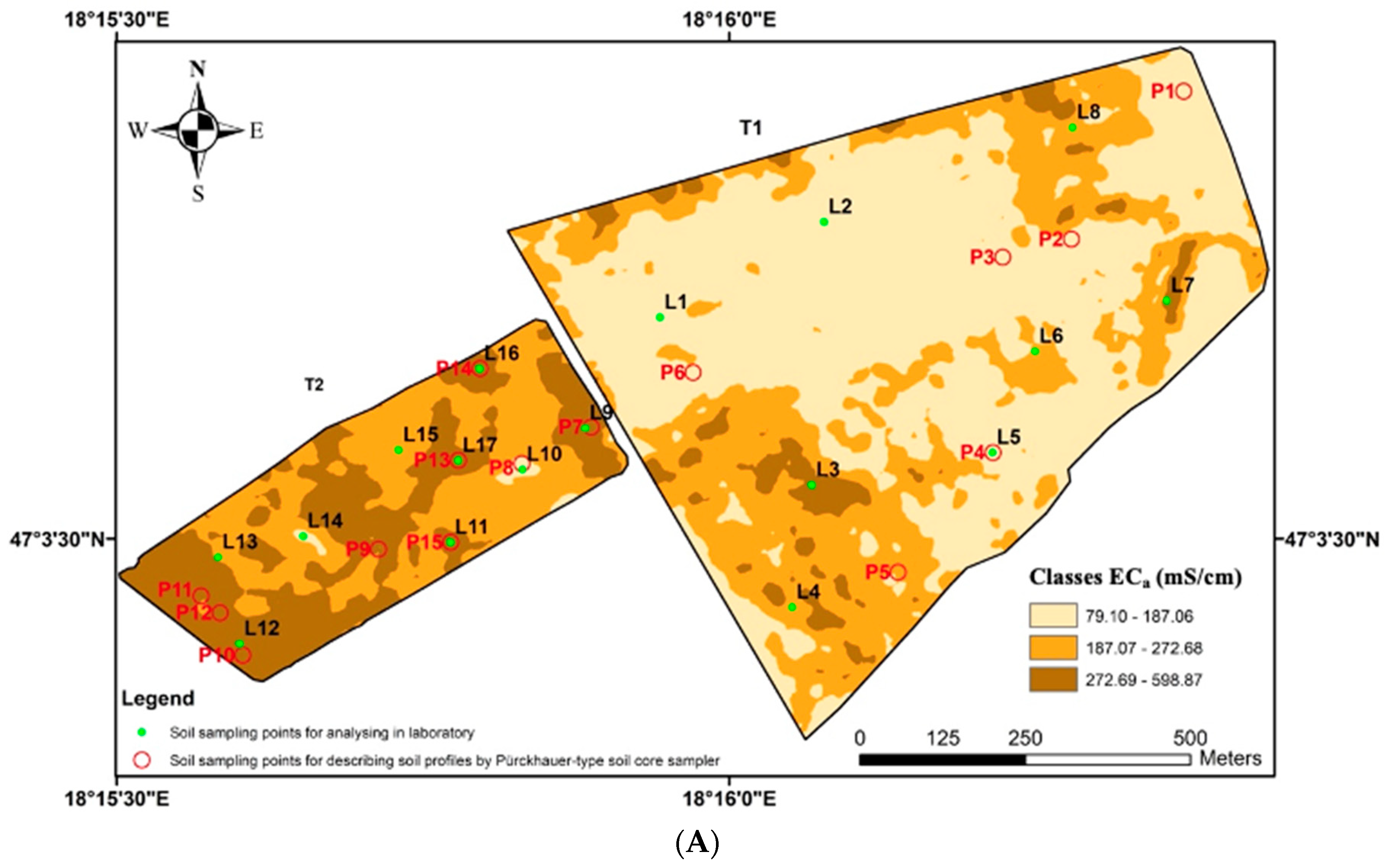
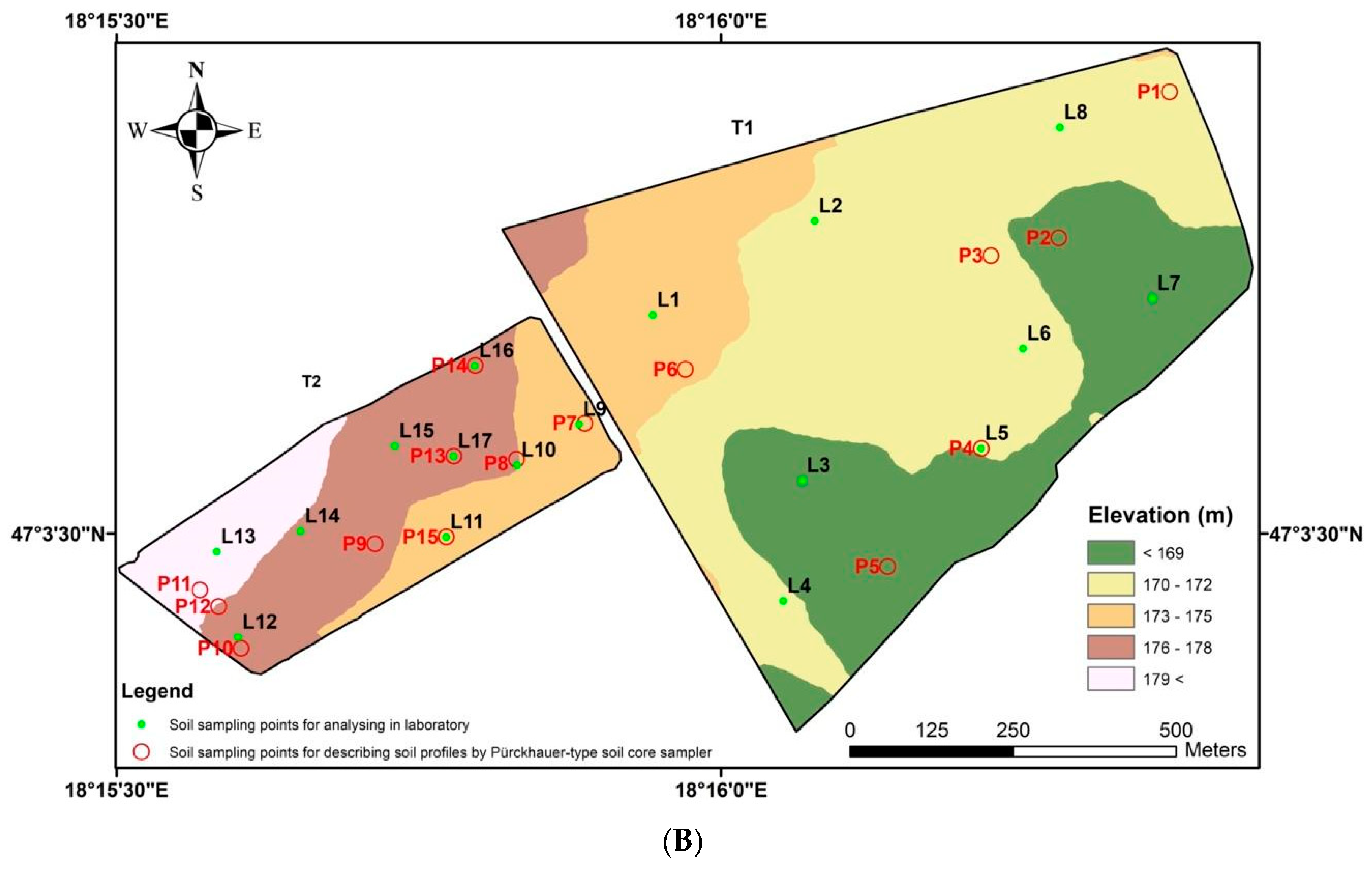
2.1. Experimental Sites
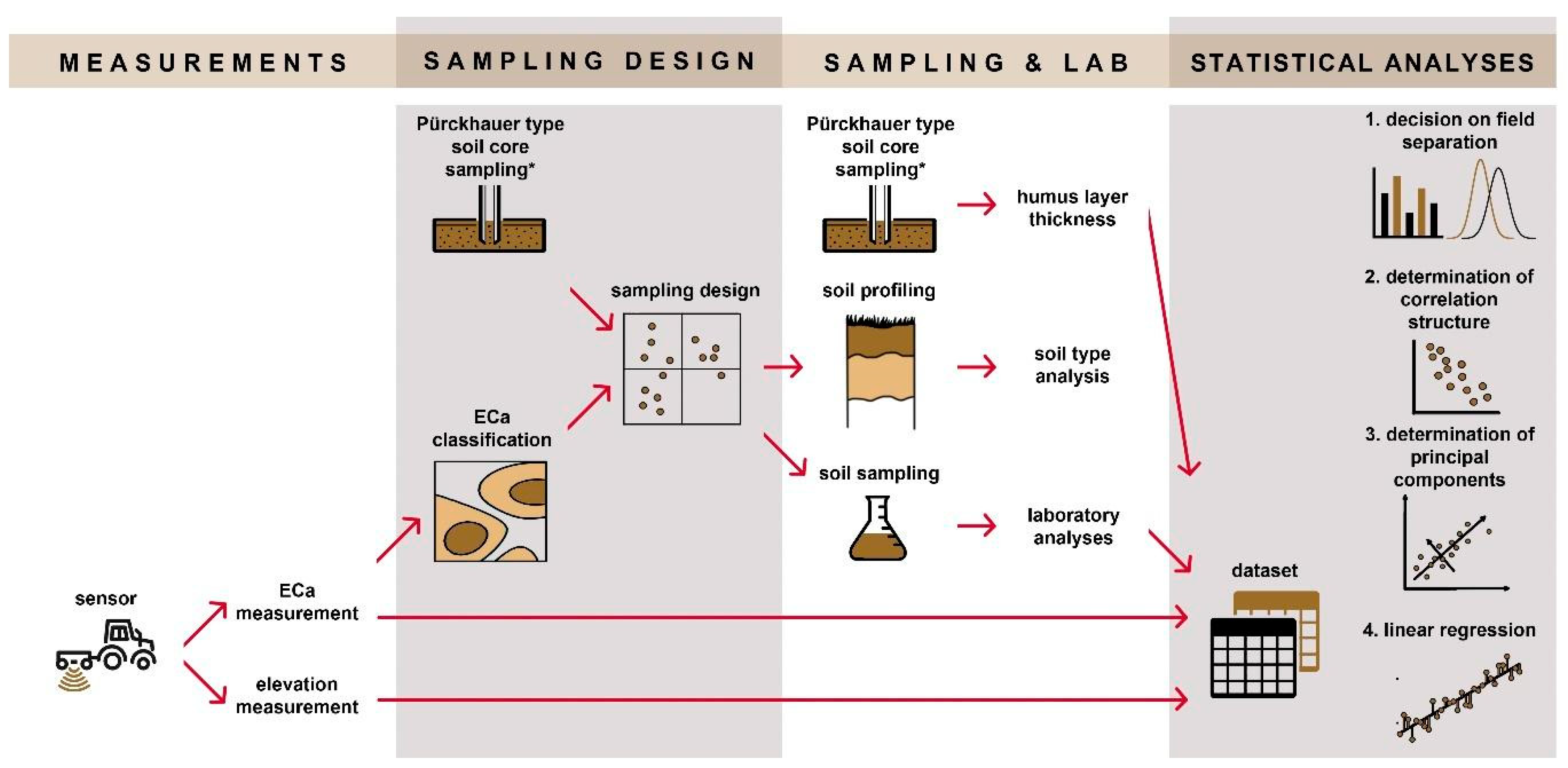
2.2. Field Measurements
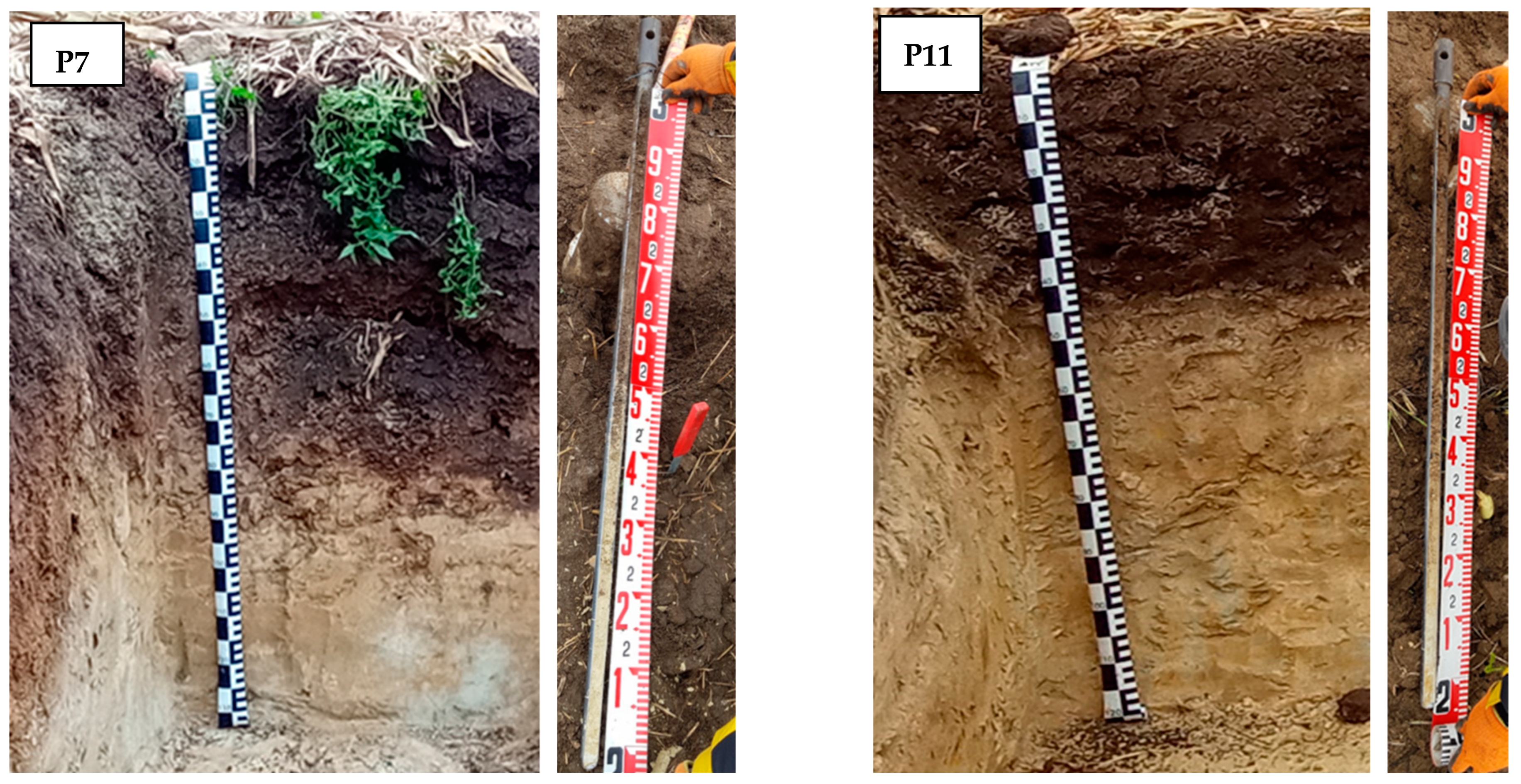
2.2.1. In Situ Data Collection
2.2.2. Soil Sampling and Analysis
- Laboratory ECa (ECa-lab);
- Nitrate, nitrite (KCl soluble);
- P2O5 (ammonium–lactate soluble);
- K2O (ammonium–lactate soluble);
- Sulphate (KCl soluble);
- Magnesium (KCl soluble);
- Sodium (KCl soluble);
- Copper EDTA (KCl-EDTA soluble);
- Manganese (KCl-EDTA soluble);
- Zinc (KCl-EDTA soluble);
- CaCO3 (Scheibler volumetric method);
- Soil organic matter—SOM (wet combustion, Turin method);
- Salt (water-soluble);
- pH (KCl, potentiometric method;
- Arany-type texture;
- Particle size distribution (Laser diffractometry, Fritsch Analysette 22 Microtech Plus).
2.3. Database Setup
2.4. Statistical Analyses
3. Results and Discussion
3.1. Comparison of the Two Fields
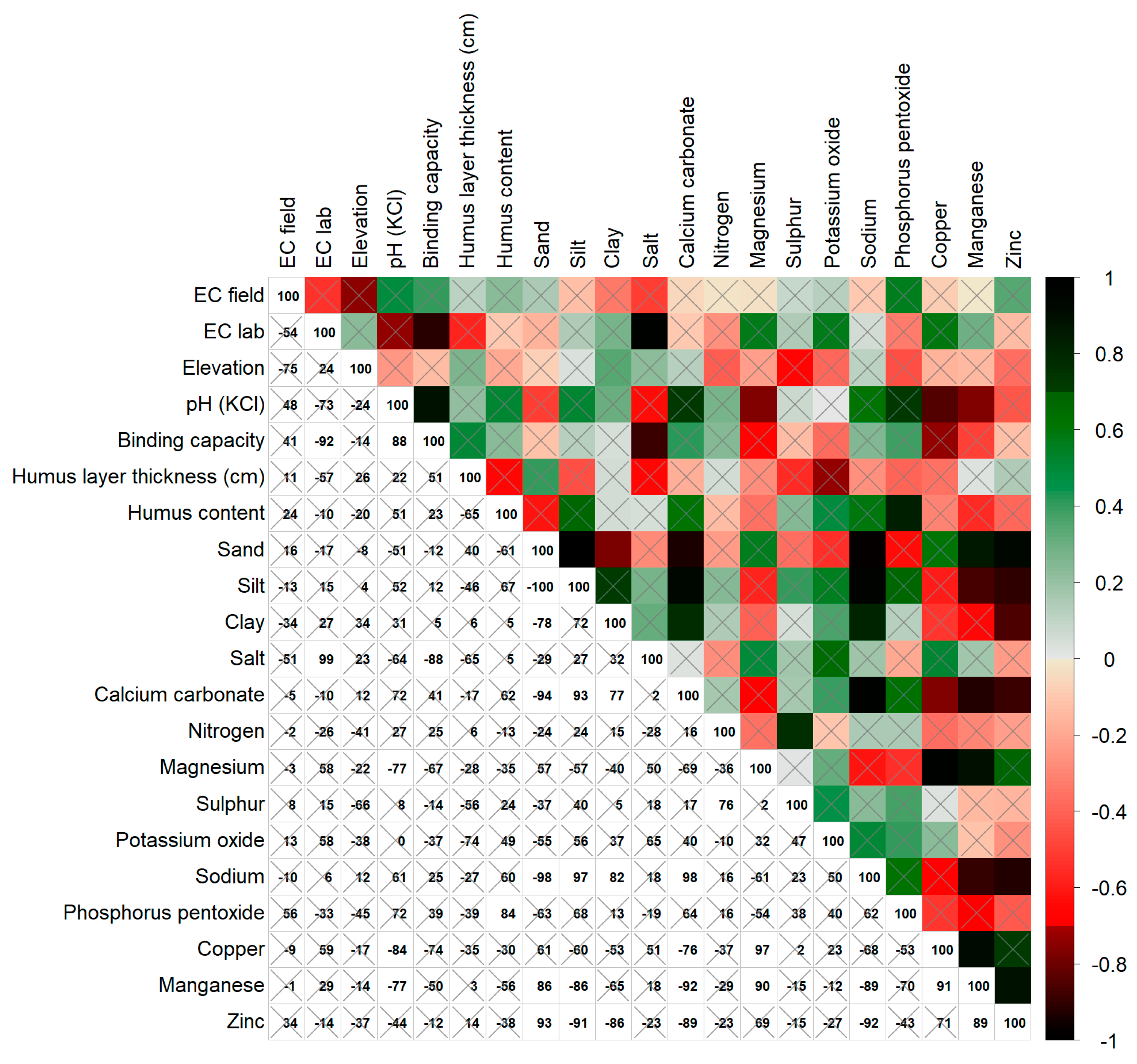
3.2. The Pearson Correlation Analysis—Relationships among ECa-field and Soil Properties
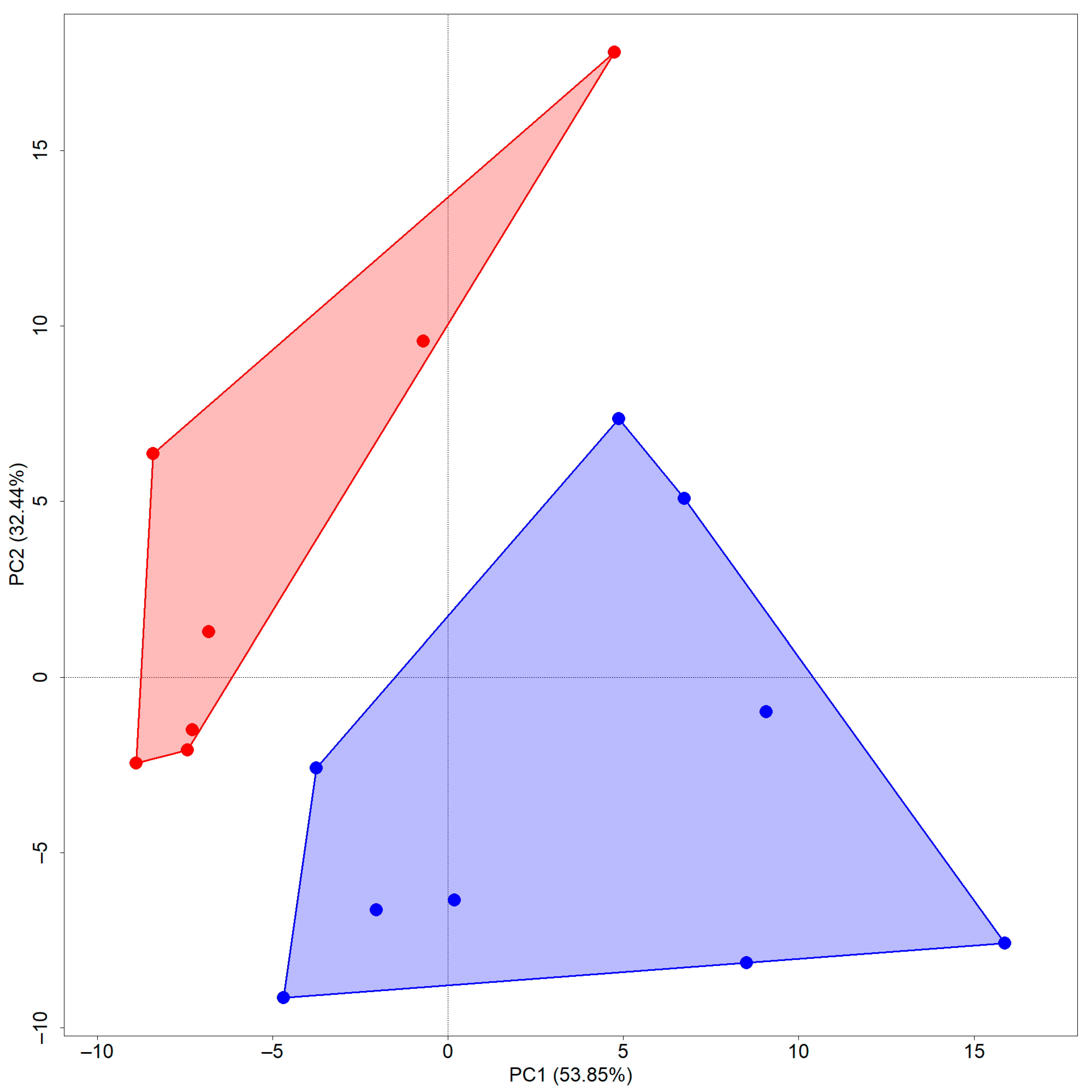
3.3. Principal Component and Regression Analyses
4. Conclusions
- Our research indicated that the relationships between the soil’s physical and chemical properties and soil apparent electrical conductivity (ECa) can vary even between two neighbouring fields. While strong correlations were found in the T2 field, weak correlations were observed in the T1 field between soil properties and ECa-field measurements. The only difference between the experimental fields was topographic variability, which was found to be a key factor in determining the relationship between ECa and soil properties, and therefore, how we interpret and use ECa for soil studies;
- Based on our results, in the absence of the relationship between the ECa-field and the soil’s physical and chemical properties, measurements based on apparent soil electrical conductivity are not suitable for characterising soil or establishing management zones. Accordingly, ECa might replace labour and time-consuming field measurements in practice only if this relationship is strong, but further experiments are required to support these findings [27,66,84];
- According to our hypothesis, ECa-based soil mapping can only be used to characterise soil and delineate management zones under homogeneous topographic conditions. To support this finding, implementing further targeted field-plot experiments with a fine-resolution grid soil sampling strategy is recommended.
Author Contributions
Funding
Data Availability Statement
Acknowledgments
Conflicts of Interest
References
- Horváth, A. A Mezőföldi Löszvegetáció Términtázati Szerveződése; Scientia Kiadó: Budapest, Hungary, 2002; pp. 1–175. (In Hungarian) [Google Scholar]
- Ádám, L.; Marosi, S.; Szilárd, J. A Mezőföld Természeti Földrajza; Akadémiai Kiadó: Budapest, Hungary, 1959; pp. 1–514. (In Hungarian) [Google Scholar]
- Hutengs, C.; Seidel, M.; Oertel, F.; Ludwig, B.; Vohland, M. In situ and laboratory soil spectroscopy with portable visible-to-near-infrared and mid-infrared instruments for the assessment of organic carbon in soils. Geoderma 2019, 355, 113900. [Google Scholar] [CrossRef]
- Watson, H.D.; Neely, H.L.; Morgan, C.L.S.; McInnes, K.J.; Molling, C.C. Identifying subsoil variation associated with gilgai using electromagnetic induction. Geoderma 2017, 295, 34–40. [Google Scholar] [CrossRef]
- Vitharana, U.; Van-Meirvenne, M.; Simpson, D.; Cocks, L.; De-Baerdemaeker, J. Key soil and topographic properties to delineate potential management classes for precision agriculture in the European loess area. Geoderma 2008, 143, 206–215. [Google Scholar] [CrossRef]
- Adamchuk, V.; Lund, E.D.; Sethuramasamyraja, B.; Morgan, M.; Dobermann, A.; Marx, D. Direct measurement of soil chemical properties on-the-go using ion-selective electrodes. Comput. Electron. Agric. 2005, 48, 272–294. [Google Scholar] [CrossRef]
- Corwin, D.L.; Lesch, S.M. Characterizing soil spatial variability with apparent soil electrical conductivity: Part II. Case study. Comput. Electron. Agric. 2005, 46, 135–152. [Google Scholar] [CrossRef]
- Friedman, S.P. Soil properties influencing apparent electrical conductivity: A review. Comput. Electron. Agric. 2005, 46, 45–70. [Google Scholar] [CrossRef]
- Nocco, M.A.; Zipper, S.C.; Booth, E.G.; Cummings, C.R.; Loheide, S.P.I.I.; Kucharik, C.J. Combining Evapotranspiration and Soil Apparent Electrical Conductivity Mapping to Identify Potential Precision Irrigation Benefits. Remote Sens. 2019, 11, 2460. [Google Scholar] [CrossRef]
- Goovaerts, P. Geostatistical tools for characterizing the spatial variability of microbiological and physico-chemical soil properties. Biol. Fertil. Soils 1998, 27, 315–334. [Google Scholar] [CrossRef]
- Jenny, H. Factors of Soil Formation: A System of Quantitative Pedology; McGraw-Hill Book Company Inc.: New York, NY, USA, 1944; pp. 1–320. [Google Scholar]
- Tsegaye, T.; Hill, R.L. Intensive tillage effects on spatial variability of soil test, plant growth, and nutrient uptake measurements. Soil Sci. 1998, 163, 155–165. [Google Scholar] [CrossRef]
- Robert, P. Characterization of soil conditions at the field level for soil specific management. Geoderma 1993, 60, 57–72. [Google Scholar] [CrossRef]
- Cook, S.E.; Corner, R.J.; Grealish, G.; Gessler, P.E.; Chartres, C.J. A rule-based system to map soil properties. Soil Sci. Soc. Am. J. 1996, 60, 1893–1900. [Google Scholar] [CrossRef]
- Mallarino, A.P.; Wittry, D.J. Efficacy of grid and zone soil sampling approaches for site-specific assessment of phosphorus, potassium, pH, and organic matter. Precis. Agric. 2004, 5, 131–144. [Google Scholar] [CrossRef]
- Prado, E.V.; Machado, T.A.; Prado, F.M.T. Geração e correlação de zonas de manejo usando sensor spad e condutividade elétrica aparente do solo para a cafeicultura irrigada na zona da mata mineira. Rev. Científica Eletrônica Agron. 2015, 1, 1–7. (In Spanish) [Google Scholar]
- Gonçalves, J.R.M.R.; Ferraz, G.A.E.S.; Reynaldo, É.F.; Marin, D.B.; Ferraz, P.F.P.; Pérez-Ruiz, M.; Rossi, G.; Vieri, M.; Sarri, D. Comparative analysis of soil-sampling methods used in precision agriculture. J. Agric. Eng. 2021, 52, 1117. [Google Scholar] [CrossRef]
- Corwin, D.L.; Lesch, S. Application of soil electrical conductivity to precision agriculture: Theory, principles and guidelines. Agron. J. 2003, 95, 455–471. [Google Scholar] [CrossRef]
- Corwin, D.L.; Lesch, S.M.; Shouse, P.J.; Soppe, R.; Ayars, J.E. Identifying soil properties that influence cotton yield using soil sampling directed by apparent soil electrical conductivity. Agron. J. 2003, 95, 352–364. [Google Scholar] [CrossRef]
- Corwin, D.L.; Scudiero, E. Field-scale apparent soil electrical conductivity of soil analysis field-scale apparent soil electrical conductivity. In Methods of Soil Analysis; Logsdon, S., Ed.; Soil Science Society of America: Madison, WI, USA, 2016; pp. 1–29. [Google Scholar]
- Doolittle, J.; Stuebe, A.; Price, A.; Kelly, E. Mapping bedrock depths with electromagnetic induction in Costilla County, Colorado. Soil Surv. Horiz. 2015, 43, 14–21. [Google Scholar] [CrossRef]
- Lesch, S.M.; Corwin, D.L.; Robinson, D.A. Apparent soil electrical conductivity mapping as an agricultural management tool in arid zone soils. Comput. Electron. Agric. 2005, 46, 351–378. [Google Scholar] [CrossRef]
- Lesch, S.M.; Rhoades, J.D.; Corwin, D.L. ESAP-95 Version 2.10R: User Manual and Tutorial Guide; Research Report; USDA-ARS, US Salinity Laboratory: Riverside, CA, USA, 2000; p. 146.
- Paz, A.M.; Castanheira, N.; Farzamian, M.; Paz, M.C.; Gonçalves, M.C.; Santos, F.A.M.; Triantafilis, J. Prediction of soil salinity and sodicity using electromagnetic conductivity imaging. Geoderma 2020, 361, 114086. [Google Scholar] [CrossRef]
- Rhoades, J.D.; Raats, P.A.C.; Prather, R.J. Effects of liquid-phase electrical conductivity, water content, and surface conductivity on bulk soil electrical conductivity. Soil Sci. Soc. Am. J. 1976, 40, 651–655. [Google Scholar] [CrossRef]
- Fortes, R.; Millán, S.; Prieto, M.H.; Torres, C.C. A methodology based on apparent electrical conductivity and guided soil samples to improve irrigation zoning. Precis. Agric. 2015, 16, 441–454. [Google Scholar] [CrossRef]
- Moral, F.J.; Terrón, J.M.; da Silva, J.R.M. Delineation of management zones using mobile measurements of soil apparent electrical conductivity and multivariate geostatistical techniques. Soil Tillage Res. 2010, 106, 335–343. [Google Scholar] [CrossRef]
- Williams, B.G.; Hoey, D. The use of electromagnetic induction to detect the spatial variability of the salt and clay contents of soils. Aust. J. Soil Res. 1987, 25, 21–27. [Google Scholar] [CrossRef]
- Rhoades, J.D.; Corwin, D.L.; Lesch, S.M. Geospatial measurements of soil electrical conductivity to determine soil salinity and diffuse salt loading from irrigation. In Assessment of Non-Point Source Pollution in the Vadose Zone; Corwin, D.L., Loague, K., Ellsworth, T.R., Eds.; American Geophysical Union: Washington, DC, USA, 1999; pp. 197–215. [Google Scholar] [CrossRef]
- Greenhouse, J.P.; Slaine, D.D. The use of reconnaissance electromagnetic methods to map contaminant migration. Groundw. Monit. Rev. 1983, 3, 47–59. [Google Scholar] [CrossRef]
- Kitchen, N.R.; Sudduth, K.A.; Drummond, S.T. Characterizing Soil Physical and Chemical Properties Influencing Crop Yield Using Soil Electrical Conductivity; ERIM International: Ann Arbor, MI, USA, 2000; pp. 122–131. [Google Scholar]
- McBride, R.A.; Shrive, S.C.; Gordon, A.M. Estimating Forest Soil Quality from Terrain Measurements of Apparent Electrical Conductivity. Soil Sci. Soc. Am. J. 1990, 54, 290–293. [Google Scholar] [CrossRef]
- Kühn, J.; Brenning, A.; Wehrhan, M.; Koszinski, S.; Sommer, M. Interpretation of electrical conductivity patterns by soil properties and geological maps for precision agriculture. Precis. Agric. 2009, 10, 490–507. [Google Scholar] [CrossRef]
- Corwin, D.L.; Ahmad, H.R. Spatio-temporal impacts of dairy lagoon water reuse on soil: Heavy metals and salinity. Environ. Sci. Process. Impacts 2015, 17, 1731–1748. [Google Scholar] [CrossRef] [PubMed]
- Bekele, A.; Hudnall, W.H.; Daigle, J.J.; Prudente, J.A.; Wolcott, M. Scale dependent variability of soil electrical conductivity by indirect measures of soil properties. J. Terramech. 2005, 42, 339–351. [Google Scholar] [CrossRef]
- Fenton, T.E.; Lauterbach, M.A. Soil map unit composition and scale of mapping related to interpretations for precision soil and crop management in Iowa. In Proceedings of the Fourth International Conference on Precision Agriculture, St. Paul, MN, USA, 19–22 July 1998; Robert, P.C., Rust, R.H., Larson, W.E., Eds.; ASA, CSSA, and SSSA Books: Madison, WI, USA, 1999; pp. 295–341. [Google Scholar]
- Peralta, N.R.; Costa, J.L.; Balzarini, M.; Angelini, H. Delineation of management zones with measurements of soil apparent electrical conductivity in the southeastern pampas. Can. J. Soil Sci. 2013, 93, 205–218. [Google Scholar] [CrossRef]
- Corwin, D.L.; Lesch, S.M. Protocols and guidelines for field-scale measurement of soil salinity distribution with ECa–directed soil sampling. J. Environ. Eng. Geophys. 2013, 18, 1–25. [Google Scholar] [CrossRef]
- Sudduth, K.A.; Kitchen, N.R.; Wiebold, W.J.; Batchelor, W.D.; Bollero, G.A.; Bullock, D.G.; Clay, D.E.; Palm, H.L.; Pierce, F.J.; Schuler, R.T.; et al. Relating apparent electrical conductivity top soil properties across the North-Central USA. Comput. Electron. Agric. 2005, 46, 263–283. [Google Scholar] [CrossRef]
- Córdoba, M.A.; Bruno, C.I.; Costa, J.L.; Peralta, N.R.; Balzarini, M.G. Protocol for multivariate homogeneous zone delineation in precision agriculture. Biosyst. Eng. 2016, 143, 95–107. [Google Scholar] [CrossRef]
- Fridgen, J.J.; Kitchen, N.R.; Sudduth, K.A.; Drummond, S.T.; Wiebold, W.J.; Fraisse, C.W. Management zone analyst (MZA): Software for subfield management zone delineation. Agron. J. 2004, 96, 100–108. [Google Scholar] [CrossRef]
- Kitchen, N.R.; Sudduth, K.A.; Myersb, D.B.; Drummonda, S.T.; Hongc, S.Y. Delineating productivity zones on claypan soil fields using apparent soil electrical conductivity. Comput. Electron. Agric. 2005, 46, 285–308. [Google Scholar] [CrossRef]
- Ortega, R.A.; Santibáňez, O.A. Determination of management zones in corn (Zea mays L.) based on soil fertility. Comput. Electron. Agric. 2007, 58, 49–59. [Google Scholar] [CrossRef]
- Xin-Zhoung, W.; Guo-Shun, L.; Hong-Chao, H.; Zhen-Hai, W.; Qing-Hua, L.; Xu-Feng, L.; Wei-Hong, H.; Yan-Tao, L. Determination of management zones for a tobacco field based on soil fertility. Comput. Electron. Agric. 2009, 65, 168–175. [Google Scholar] [CrossRef]
- Singh, G.; Williard, K.W.J.; Schoonover, J.E. Spatial relation of Apparent soil electrical conductivity with crop yield and soil properties at different topographic positions in a small agricultural watershed. Agronomy 2016, 6, 57. [Google Scholar] [CrossRef]
- Zhu, Q.; Lin, H. Repeated electromagnetic induction surveys for determining subsurface hydrologic dynamics in an agricultural landscape. Soil Sci. Soc. Am. J. 2010, 74, 1750–1762. [Google Scholar] [CrossRef]
- Marosi, S.; Somogyi, S. Magyarország Kistájainak Katasztere, I–II; MTA-Földrajztudományi Kutató Intézet: Budapest, Hungary, 1990; pp. 1–1023. (In Hungarian) [Google Scholar]
- Rhoades, J.D.; Ingvalson, R.D. Determining Salinity in Field Soils with Soil Resistance Measurements. Soil Chem. 1971, 35, 54–60. [Google Scholar] [CrossRef]
- Rhoades, J.D.; Manteghi, N.A.; Shouse, P.J.; Alves, W.J. Soil Electrical Conductivity and Soil Salinity: New Formulations and Calibrations. Soil Sci. Soc. Am. J. 1989, 53, 433–439. [Google Scholar] [CrossRef]
- Peralta, N.R.; Costa, J.L. Delineation of management zones with soil apparent electrical conductivity to improve nutrient management. Comput. Electron. Agric. 2013, 99, 218–226. [Google Scholar] [CrossRef]
- Finnern, H.; Grottenthaler, W.; Kühn, D.; Palchen, W.; Schraps, W.G.; Sponagel, H. Kartieranleitung. 4. Verbesserte und Erweiterte Auflage; AG Boden: Hannover, Germany, 1994. (In German) [Google Scholar]
- Buzás, I.; Daróczi, S.; Dódony, I.; Kálmán, A.; Kocsis, I.; Pártay, G.; Rajkai, K. Talaj-És Agrokémiai Vizsgálati Módszerkönyv 1; Inda 4231 Kiadó: Budapest, Hungary, 1993. (In Hungarian) [Google Scholar]
- Team, R.C. R: A Language and Environment for Statistical Computing, R Foundation for Statistical Computing; R-Project: Vienna, Austria, 2018.
- Fox, J.; Weisberg, S. An R Companion to Applied Regression, 3rd ed.; SAGE Publications, Inc.: Thousand Oaks, CA, USA, 2019. [Google Scholar]
- Wei, T.; Simko, V. R Package “Corrplot”: Visualization of a Correlation Matrix, Version 0.84; R-Project: Vienna, Austria, 2017.
- Oksanen, J.; Blanchet, F.G.; Kindt, R.; Legendre, P.; Minchin, P.R.; O’Hara, R.B.; Simpson, G.L.; Solymos, P.; Stevens, M.H.M.; Wagner, H. Vegan: Community Ecology Package, R package Version 2.3-4; R-Project: Vienna, Austria, 2019.
- Riley, S.J.; DeGloria, S.D.; Elliot, R. A terrain ruggedness index that quantifies topographic heterogeneity. Intermt. J. Sci. 1999, 5, 23–27. [Google Scholar]
- Wilson, M.F.J.; O’Connell, B.; Brown, C.; Guinan, J.C.; Grehan, A.J. Multiscale terrain analysis of multibeam bathymetry data for habitat mapping on the continental slope. Mar. Geod. 2007, 30, 3–35. [Google Scholar] [CrossRef]
- Pearson, K. On lines and planes of closest fit to systems of points in space. Lond. Edinb. Dublin Philos. Mag. J. Sci. 1901, 2, 559–572. [Google Scholar] [CrossRef]
- Hotelling, H. Analysis of a complex of statistical variables into principal components. J. Educ. Psychol. 1933, 24, 417–441. [Google Scholar] [CrossRef]
- Sharma, S. Applied Multivariate Techniques; John Wiley and Sons: New York, NY, USA, 1996. [Google Scholar]
- Boecker, D.; Centeri, C.; Welp, G.; Möseler, B.M. Parallels of secondary grassland succession and soil regeneration in a chronosequence of central-Hungarian old fields. Folia Geobot. 2015, 50, 91–106. [Google Scholar] [CrossRef]
- Jassó, F.; Darab, K.; Fórizsa, J.-N.; Földvári, G.; Várallyay, G. A Genetikus Üzemi Talajtérképezés Módszerkönyve; Országos Mezőgazdasági Minőségvizsgáló Intézet: Budapest, Hungary, 1966; pp. 509–510. (In Hungarian) [Google Scholar]
- Stefanovits, P.; Filep, G.; Füleky, G. Talajtan; Mezőgazda Kiadó: Budapest, Hungary, 2010; pp. 1–433. (In Hungarian) [Google Scholar]
- Michéli, E.; Fuchs, M.; Hegymegi, P.; Stefanovits, P. Classification of the major soils of Hungary and their correlation with the world reference base for soil resources (WRB). Agrokémia És Talajt. 2006, 55, 19–28. [Google Scholar] [CrossRef]
- Fraisse, C.W.; Sudduth, K.A.; Kitchen, N.R. Delineation of site-specific management zones by unsupervised classification of topographic attributes and soil electrical conductivity. Am. Soc. Agric. Biol. Eng. 2001, 44, 155–166. [Google Scholar] [CrossRef]
- Ayele, G.T.; Demissie, S.S.; Jemberrie, M.A.; Jeong, J.; Hamilton, D.P. Terrain effects on the spatial variability of soil physical and chemical properties. Soil Syst. 2019, 4, 1. [Google Scholar] [CrossRef]
- Bakr, N.; Ali, R.R. Statistical relationship between land surface altitude and soil salinity in the enclosed desert depression of arid regions. Arab. J. Geosci. 2019, 12, 715. [Google Scholar] [CrossRef]
- Heiniger, R.W.; McBride, R.G.; Clay, D.E. Using soil electrical conductivity to improve nutrient management. Agron. J. 2003, 95, 508–519. [Google Scholar] [CrossRef]
- Moore, I.D.; Gessler, P.; Nielsen, G.; Peterson, G. Soil attribute prediction using terrain analysis. Soil Sci. Soc. Am. J. 1993, 57, 443–452. [Google Scholar] [CrossRef]
- Heil, K.; Schmidhalter, U. Characterisation of soil texture variability using the apparent soil electrical conductivity at a highly variable site. Comput. Geosci. 2012, 39, 98–110. [Google Scholar] [CrossRef]
- Carroll, Z.; Oliver, M. Exploring the spatial relations between soil physical properties and apparent electrical conductivity. Geoderma 2005, 128, 354–374. [Google Scholar] [CrossRef]
- Nyéki, A.; Milics, G.; Kovács, A.J.; Neményi, M. Effects of soil compaction on cereal yield. Cereal Res. Commun. 2017, 45, 1–22. [Google Scholar] [CrossRef]
- Broge, N.H.; Thomsen, A.G.; Greve, M.H. Prediction of topsoil organic matter and clay content from measurements of spectral reflectance and electrical conductivity. Acta Agric. Scand. Sect. B Soil Plant Sci. 2006, 54, 232–240. [Google Scholar] [CrossRef]
- Rezaei, M.; Saey, T.; Seuntjens, P.; Joris, I.; Boënne, W.; Meirvenne, M.V.; Cornelis, W. Predicting saturated hydraulic conductivity in a sandy grassland using proximally sensed apparent electrical conductivity. J. Appl. Geophys. 2016, 126, 35–41. [Google Scholar] [CrossRef]
- Bronson, K.F.; Booker, J.D.; Officer, S.J.; Lascano, R.J.; Maas, S.J.; Searcy, S.W. Apparent electrical conductivity, soil properties and spatial covariance in the U.S. Southern High Plains. Precis. Agric. 2005, 6, 297–311. [Google Scholar] [CrossRef]
- Omonode, R.A.; Vyn, T.J. Spatial dependence and relationships of electrical conductivity to soil organic matter, phosphorus, and potassium. Soil Sci. 2006, 171, 223–238. [Google Scholar] [CrossRef]
- Serrano, J.; Shahidian, S.; Silva, J.M.D. Spatial and Temporal Patterns of Apparent Electrical Conductivity: DUALEM vs. Veris Sensors for Monitoring Soil Properties. Sensors 2014, 14, 10024–10041. [Google Scholar] [CrossRef]
- Lal, R. Soil carbon sequestration impacts on global climate change and food security. Science 2004, 304, 1623–1627. [Google Scholar] [CrossRef] [PubMed]
- Martinez, G.; Vanderlinden, K.; Giráldez, J.V.; Espejo, A.J.; Muriel, J.L. Field-scale soil moisture pattern mapping using electromagnetic induction. Vadose Zone J. 2010, 9, 871–881. [Google Scholar] [CrossRef]
- Reyes, J.; Wendroth, O.; Matocha, C.; Zhu, J. Delineating site-specific management zones and evaluating soil water temporal dynamics in a farmer’s field in Kentucky. Vadose Zone J. 2019, 18, 1–19. [Google Scholar] [CrossRef]
- Van Meirvenne, M.; Islam, M.M.; De Smedt, P.; Meerschman, E.; Van De Vijver, E.; Saey, T. Key variables for the identification of soil management classes in the Aeolian landscapes of north–west Europe. Geoderma 2013, 199, 99–105. [Google Scholar] [CrossRef]
- Peralta, N.R.; Costa, J.L.; Balzarini, M.; Franco, M.C.; Córdoba, M.; Bullock, D. Delineation of management zones to improve nitrogen management of wheat. Comput. Electron. Agric. 2015, 110, 103–113. [Google Scholar] [CrossRef]
- Li, Y.; Shi, Z.; Li, F. Delineation of site-specific management zones based on temporal and spatial variability of soil electrical conductivity. Pedosphere 2007, 17, 156–164. [Google Scholar] [CrossRef]
- Johnson, C.K.; Doran, J.W.; Duke, H.R.; Wienhold, B.; Eskridge, K.; Shanahan, J. Field-scale electrical conductivity mapping for delineating soil condition. Soil Sci. Soc. Am. J. 2001, 65, 1829–1837. [Google Scholar] [CrossRef]
- Sudduth, K.A.; Kitchen, N.R.; Bollero, G.A.; Bullock, D.G.; Wiebold, W.J. Comparison of electromagnetic induction and direct sensing of soil electrical conductivity. Agron. J. 2003, 95, 472–482. [Google Scholar] [CrossRef]


| Field | Variables | Mean | Median | SD | CV | Min | Max | Range |
|---|---|---|---|---|---|---|---|---|
| T1 | ECa-field (mS/cm) | 223.75 | 241.37 | 69.37 | 0.31 | 114.38 | 321.35 | 206.97 |
| ECa-lab (mS/cm) | 476.57 | 465.00 | 36.98 | 0.08 | 417.00 | 532.00 | 115.00 | |
| Elevation (m) | 169.00 | 169.18 | 1.75 | 0.01 | 166.49 | 170.80 | 4.31 | |
| pH (KCl) | 7.00 | 7.19 | 0.44 | 0.06 | 6.15 | 7.37 | 1.22 | |
| Binding capacity (KA) | 49.86 | 50.00 | 2.67 | 0.05 | 45.00 | 53.00 | 8.00 | |
| Humus layer thickness (cm) | 39.29 | 35.00 | 7.87 | 0.20 | 35.00 | 55.00 | 20.00 | |
| SOM (% by weight) | 2.13 | 2.00 | 0.39 | 0.18 | 1.60 | 2.70 | 1.10 | |
| Sand (%) | 16.66 | 16.31 | 6.37 | 0.38 | 9.77 | 26.05 | 16.29 | |
| Silt (%) | 77.42 | 78.34 | 5.76 | 0.07 | 68.70 | 83.80 | 15.10 | |
| Clay (%) | 5.92 | 5.72 | 0.81 | 0.14 | 5.25 | 7.50 | 2.25 | |
| Salt (% by weight) | 0.03 | 0.03 | 0.01 | 0.38 | 0.01 | 0.05 | 0.04 | |
| CaCO3 (% by weight) | 5.63 | 7.40 | 5.58 | 0.99 | 0.00 | 12.30 | 12.30 | |
| N (mg/kg) | 10.14 | 10.00 | 2.04 | 0.20 | 7.00 | 13.00 | 6.00 | |
| Mg (mg/kg) | 295.00 | 241.00 | 132.56 | 0.45 | 191.00 | 557.00 | 366.00 | |
| S (mg/kg) | 2.87 | 2.90 | 0.42 | 0.15 | 2.40 | 3.40 | 1.00 | |
| K2O (mg/kg) | 253.57 | 266.00 | 47.35 | 0.19 | 159.00 | 305.00 | 146.00 | |
| Na (mg/kg) | 29.00 | 31.00 | 11.80 | 0.41 | 14.00 | 44.00 | 30.00 | |
| P2O5 (mg/kg) | 56.29 | 53.00 | 22.51 | 0.40 | 29.00 | 93.00 | 64.00 | |
| Cu (mg/kg) | 1.51 | 1.20 | 0.74 | 0.49 | 0.90 | 2.80 | 1.90 | |
| Mn (mg/kg) | 159.71 | 128.00 | 95.57 | 0.60 | 71.00 | 315.00 | 244.00 | |
| Zn (mg/kg) | 0.59 | 0.60 | 0.21 | 0.36 | 0.30 | 0.90 | 0.60 | |
| T2 | ECa-field (mS/cm) | 314.78 | 320.91 | 136.04 | 0.43 | 147.09 | 552.15 | 405.06 |
| ECa-lab (mS/cm) | 646.89 | 602.00 | 88.56 | 0.14 | 548.00 | 806.00 | 258.00 | |
| Elevation (m) | 176.05 | 176.64 | 2.28 | 0.01 | 172.61 | 179.50 | 6.89 | |
| pH (KCl) | 7.11 | 7.12 | 0.15 | 0.02 | 6.88 | 7.30 | 0.42 | |
| Binding capacity (KA) | 50.67 | 50.00 | 2.87 | 0.06 | 48.00 | 57.00 | 9.00 | |
| Humus layer thickness (cm) | 58.33 | 60.00 | 14.79 | 0.25 | 35.00 | 90.00 | 55.00 | |
| SOM (% by weight) | 1.86 | 1.80 | 0.30 | 0.16 | 1.50 | 2.50 | 1.00 | |
| Sand (%) | 15.77 | 18.73 | 7.06 | 0.45 | 2.28 | 24.38 | 22.10 | |
| Silt (%) | 77.93 | 75.69 | 6.16 | 0.08 | 70.94 | 90.32 | 19.38 | |
| Clay (%) | 6.30 | 6.19 | 1.02 | 0.16 | 4.68 | 7.52 | 2.84 | |
| Salt (% by weight) | 0.07 | 0.06 | 0.01 | 0.21 | 0.05 | 0.09 | 0.04 | |
| CaCO3 (% by weight) | 4.99 | 3.50 | 6.55 | 1.31 | 0.00 | 19.70 | 19.70 | |
| N (mg/kg) | 19.78 | 15.00 | 9.11 | 0.46 | 10.00 | 34.00 | 24.00 | |
| Mg (mg/kg) | 302.11 | 320.00 | 100.34 | 0.33 | 154.00 | 444.00 | 290.00 | |
| S (mg/kg) | 4.42 | 4.20 | 1.21 | 0.27 | 3.00 | 6.50 | 3.50 | |
| K2O (mg/kg) | 321.56 | 301.00 | 63.21 | 0.20 | 255.00 | 460.00 | 205.00 | |
| Na (mg/kg) | 36.11 | 32.00 | 14.95 | 0.41 | 23.00 | 71.00 | 48.00 | |
| P2O5 (mg/kg) | 184.00 | 183.00 | 85.34 | 0.46 | 65.00 | 365.00 | 300.00 | |
| Cu (mg/kg) | 1.94 | 1.50 | 0.89 | 0.46 | 1.00 | 3.20 | 2.20 | |
| Mn (mg/kg) | 182.00 | 133.00 | 101.38 | 0.56 | 65.00 | 321.00 | 256.00 | |
| Zn (mg/kg) | 0.93 | 0.70 | 0.47 | 0.51 | 0.50 | 1.90 | 1.40 |
| Fields | T1 | T2 | |||||
|---|---|---|---|---|---|---|---|
| PCs | PC1 | PC2 | PC3 | PC1 | PC2 | PC3 | PC4 |
| Eigenvalue | 12.78 | 3.75 | 2.11 | 9.313 | 4.003 | 3.118 | 1.978 |
| Cumulative σ2 | 63.89 | 82.64 | 93.18 | 46.565 | 66.580 | 82.171 | 92.060 |
| Parameter scores | |||||||
| ECa-lab (mS/cm) | −0.038 | 0.188 | 0.071 | 0.117 | 0.205 | −0.194 | −0.312 |
| Elevation (m) | 0.012 | 0.017 | 0.239 | −0.019 | −0.109 | −0.230 | −0.136 |
| pH (KCl) | 0.359 | −0.324 | −0.267 | −0.078 | −0.070 | −0.155 | 0.025 |
| Binding capacity (KA) | 0.150 | −0.359 | −0.119 | −0.025 | 0.147 | −0.203 | 0.460 |
| Humus layer thickness (cm) | −0.005 | −0.247 | 0.228 | −0.047 | 0.097 | 0.384 | 0.330 |
| SOM (% by weight) | 0.227 | 0.208 | −0.664 | 0.191 | 0.057 | −0.157 | 0.282 |
| Sand (%) | −0.274 | −0.289 | −0.039 | 0.161 | −0.453 | 0.006 | 0.177 |
| Silt (%) | 0.272 | 0.286 | −0.022 | −0.159 | 0.421 | −0.017 | −0.209 |
| Clay (%) | 0.217 | 0.241 | 0.488 | −0.131 | 0.586 | 0.078 | 0.113 |
| Salt (% by weight) | −0.040 | 0.326 | 0.084 | 0.122 | 0.125 | −0.159 | −0.218 |
| CaCO3 (% by weight) | 0.319 | 0.150 | 0.024 | −0.312 | 0.010 | −0.312 | 0.305 |
| N (mg/kg) | 0.025 | −0.030 | 0.030 | 0.280 | 0.017 | −0.405 | 0.253 |
| Mg (mg/kg) | −0.337 | 0.272 | −0.124 | 0.138 | 0.264 | 0.250 | 0.080 |
| S (mg/kg) | 0.019 | 0.078 | −0.083 | 0.260 | 0.135 | −0.325 | −0.163 |
| K2O (mg/kg) | 0.033 | 0.283 | −0.141 | 0.156 | 0.144 | −0.088 | −0.178 |
| Na (mg/kg) | 0.223 | 0.176 | 0.043 | −0.187 | 0.149 | −0.330 | 0.232 |
| P2O5 (mg/kg) | 0.057 | 0.010 | −0.115 | 0.245 | −0.063 | −0.126 | −0.142 |
| Cu (mg/kg) | −0.345 | 0.266 | −0.173 | 0.411 | 0.128 | 0.239 | 0.177 |
| Mn (mg/kg) | −0.436 | −0.009 | −0.077 | 0.446 | 0.072 | 0.120 | 0.086 |
| Zn (mg/kg) | −0.133 | −0.102 | −0.138 | 0.327 | 0.091 | −0.084 | 0.120 |
| Fields | Model | R2 | Adjusted R2 | RMSE |
|---|---|---|---|---|
| T1 | 0.148 + 0.013 × PC1 − 0.131 × PC2 − 0.262 × PC3 | 0.470 | 0.051 | 0.107 |
| T2 | 0.631 − 0.137 × PC1 + 0.306 × PC2 + 0.241 × PC3 − 0.281 × PC4 | 0.721 | 0.441 | 0.155 |
Disclaimer/Publisher’s Note: The statements, opinions and data contained in all publications are solely those of the individual author(s) and contributor(s) and not of MDPI and/or the editor(s). MDPI and/or the editor(s) disclaim responsibility for any injury to people or property resulting from any ideas, methods, instructions or products referred to in the content. |
© 2024 by the authors. Licensee MDPI, Basel, Switzerland. This article is an open access article distributed under the terms and conditions of the Creative Commons Attribution (CC BY) license (https://creativecommons.org/licenses/by/4.0/).
Share and Cite
Kulmány, I.M.; Bede, L.; Stencinger, D.; Zsebő, S.; Csavajda, P.; Kalocsai, R.; Vona, M.; Jakab, G.; Vona, V.M.; Bede-Fazekas, Á. Challenges in Mapping Soil Variability Using Apparent Soil Electrical Conductivity under Heterogeneous Topographic Conditions. Agronomy 2024, 14, 1161. https://doi.org/10.3390/agronomy14061161
Kulmány IM, Bede L, Stencinger D, Zsebő S, Csavajda P, Kalocsai R, Vona M, Jakab G, Vona VM, Bede-Fazekas Á. Challenges in Mapping Soil Variability Using Apparent Soil Electrical Conductivity under Heterogeneous Topographic Conditions. Agronomy. 2024; 14(6):1161. https://doi.org/10.3390/agronomy14061161
Chicago/Turabian StyleKulmány, István Mihály, László Bede, Dávid Stencinger, Sándor Zsebő, Péter Csavajda, Renátó Kalocsai, Márton Vona, Gergely Jakab, Viktória Margit Vona, and Ákos Bede-Fazekas. 2024. "Challenges in Mapping Soil Variability Using Apparent Soil Electrical Conductivity under Heterogeneous Topographic Conditions" Agronomy 14, no. 6: 1161. https://doi.org/10.3390/agronomy14061161
APA StyleKulmány, I. M., Bede, L., Stencinger, D., Zsebő, S., Csavajda, P., Kalocsai, R., Vona, M., Jakab, G., Vona, V. M., & Bede-Fazekas, Á. (2024). Challenges in Mapping Soil Variability Using Apparent Soil Electrical Conductivity under Heterogeneous Topographic Conditions. Agronomy, 14(6), 1161. https://doi.org/10.3390/agronomy14061161