Abstract
Pests have caused significant losses to agriculture, greatly increasing the detection of pests in the planting process and the cost of pest management in the early stages. At this time, advances in computer vision and deep learning for the detection of pests appearing in the crop open the door to the application of target detection algorithms that can greatly improve the efficiency of tomato pest detection and play an important technical role in the realization of the intelligent planting of tomatoes. However, in the natural environment, tomato leaf pests are small in size, large in similarity, and large in environmental variability, and this type of situation can lead to greater detection difficulty. Aiming at the above problems, a network target detection model based on deep learning, YOLONDD, is proposed in this paper. Designing a new loss function, NMIoU (Normalized Wasserstein Distance with Mean Pairwise Distance Intersection over Union), which improves the ability of anomaly processing, improves the model’s ability to detect and identify objects of different scales, and improves the robustness to scale changes; Adding a Dynamic head (DyHead) with an attention mechanism will improve the detection ability of targets at different scales, reduce the number of computations and parameters, improve the accuracy of target detection, enhance the overall performance of the model, and accelerate the training process. Adding decoupled head to Head can effectively reduce the number of parameters and computational complexity and enhance the model’s generalization ability and robustness. The experimental results show that the average accuracy of YOLONDD can reach 90.1%, which is 3.33% higher than the original YOLOv5 algorithm and is better than SSD, Faster R-CNN, YOLOv7, YOLOv8, RetinaNet, and other target detection networks, and it can be more efficiently and accurately utilized in tomato leaf pest detection.
1. Introduction
With a growing global population and accelerated urbanization, the sustainability of agricultural production has become a global challenge. Tomato is one of the most important cash crops, while tomato yield is affected by insect pests of tomato leaves, among which leafminer flies, thrips, tabacco budworm, and spider leaf mite [1,2,3] have a greater impact on tomato yield. However, traditional pest detection methods [4,5,6] rely on manual visual inspection, which is not only time-consuming and labor-intensive but also subject to subjective judgment, making it difficult to achieve wide-scale and efficient monitoring.
In recent years, deep learning has achieved significant results in pest identification [7,8,9], which can better overcome the challenges of traditional machine learning. Research on deep learning in pest detection can be categorized into two approaches: pest detection and classification and pest-induced leaf infestation feature detection. The research on pest detection and classification mainly focuses on improving the classical deep learning methods, such as P. Venk et al. [10], which achieved good results on pest datasets of three peanut crops by integrating VIT, PCA, and MFO; Pattnaik G et al. [11], which feature extraction of pests by HOG and LBP, and the extracted feature maps are fed into SVM [12] classifiers for training; In contrast, leaf damage caused by insect pests can be detected in two ways: by quantifying the extent of insect damage to the leaf and by detecting the location of the insect-damaged leaf. For example, Liang et al. [13] developed polynomial and logistic regression models for leaf extraction to estimate leaf damage; Da Silva et al. [14] used image segmentation to preserve the leaf region, augmented the dataset with a synthesis technique, and trained the network with a model for detecting pest-induced damage to leaves; Fang et al. [15], Zhu R et al. [16], Zhu L et al. [17], and others used the improved YOLO series of models to identify pest-induced leaf damage and achieved good detection results.
The detection process of pests is found to have low resolution, and small pest detection is much more difficult and less accurate than large pest detection. Therefore, the detection of small target goals is challenging in agricultural production environments. Currently, mainstream detection methods are added to the mainstream target detection model through multi-scale feature fusion, anchor frame optimization, and loss function optimization. For example, Ye et al. [18] improved YOLOv8 by proposing slice-assisted fine-tuning and slice-assisted hyper-inference (SAHI), designing a generalized efficient layer aggregation network (GELAN), introducing the MS structure, introducing the BiFormer attention mechanism, and using the MPDIoU loss function in order to solve the small targets in tea pests, and achieved a better detection effect in tea pests. Tian Y et al., [19] in order to solve insect pests in agriculture by improving the network in the feature extraction and feature fusion parts, the method is indeed feasible and has better results in the detection of small targets. However, the existing target detection algorithms still have limitations for small target pests. The occlusion and light caused by leaves, etc., bring difficulties in model detection, which affects the feature extraction ability of the network model.
In natural environments, tomato pests are small in size, large in similarity, and large in environmental variability, and these types of situations can make detection more difficult. Lippi M et al. [20], Mamdouh N et al. [21]. Yang S et al. [22]. performed algorithmic improvements based on the YOLO series for target detection of hazelnut pests, olive fruit fly, and maize pests. Their study proved that the YOLO series of algorithms has a better detection effect. Although the YOLO series of primary target detection models offers better advantages in terms of detection speed and model size, they are more suitable as benchmark models for pest detection. However, the Mosaic data augmentation used in YOLOv5 causes the originally smaller targets to become even smaller, resulting in poorer generalization ability of the model. Moreover, YOLOv5 is not very stable at detecting small targets and requires a large amount of training data to achieve high accuracy.
In response to the above issues, this paper proposes a deep learning-based target detection model, YOLONDD, for tomato leaf pest detection. The model is based on the YOLOv5 structure. Firstly, we design a new loss function NMIoU by borrowing the idea of loss function NWD and loss function MPDIoU to enhance the ability of the model to detect and recognize objects at different scales and to improve the robustness of the model. Meanwhile, we added the Dynamic head [23] module in order to improve the multi-scale feature extraction capability of the network model and to solve the challenge of too small a target in tomato leaf pest detection. Finally, we found that the number of parameters in the network model increased, and the training time was too long. In order to reduce the number of parameters and computational complexity of the network model, we introduce the Decoupled head [24] module in YOLOv5, which enhances the generalization ability and robustness of the model. The main contributions of this study include:
- We propose an improved tomato leaf pest detection model, YOLONDD, to solve the problems of uneven pest scales and low detection accuracy in the detection process.
- To enhance the ability of the model to detect and recognize objects at different scales, we design a new loss function NMIoU, which is adaptive to changes in different scales. This loss function enhances the model’s detection and recognition of small targets in the feature map.
- In order to better extract the feature information of small targets, we add the Dynamic head module, which gradually extracts the information of the feature map through the scale-aware module, spatial-aware module, and task-aware module. This method can adaptively adjust the size of the sensing field to adapt to the scale change in different targets and improve the detection ability of different scale targets.
- In order to reduce the number of parameters and training time of the model, we introduce the decoupling head module, the decoupling head helps the model to extract the target location and category information, learn the feature map information, and fuse it through different network branches, so that the model’s generalization ability and robustness are enhanced.
In addition, in order to verify the robustness of the proposed method, experiments were conducted using tomato pest images as well as infestation images in a real environment. The experimental results show that the method proposed in this paper is able to meet the requirements in terms of accuracy and other aspects of the dataset and has a better detection effect on tomato pest images.
2. Materials and Methods
2.1. Main Ideas
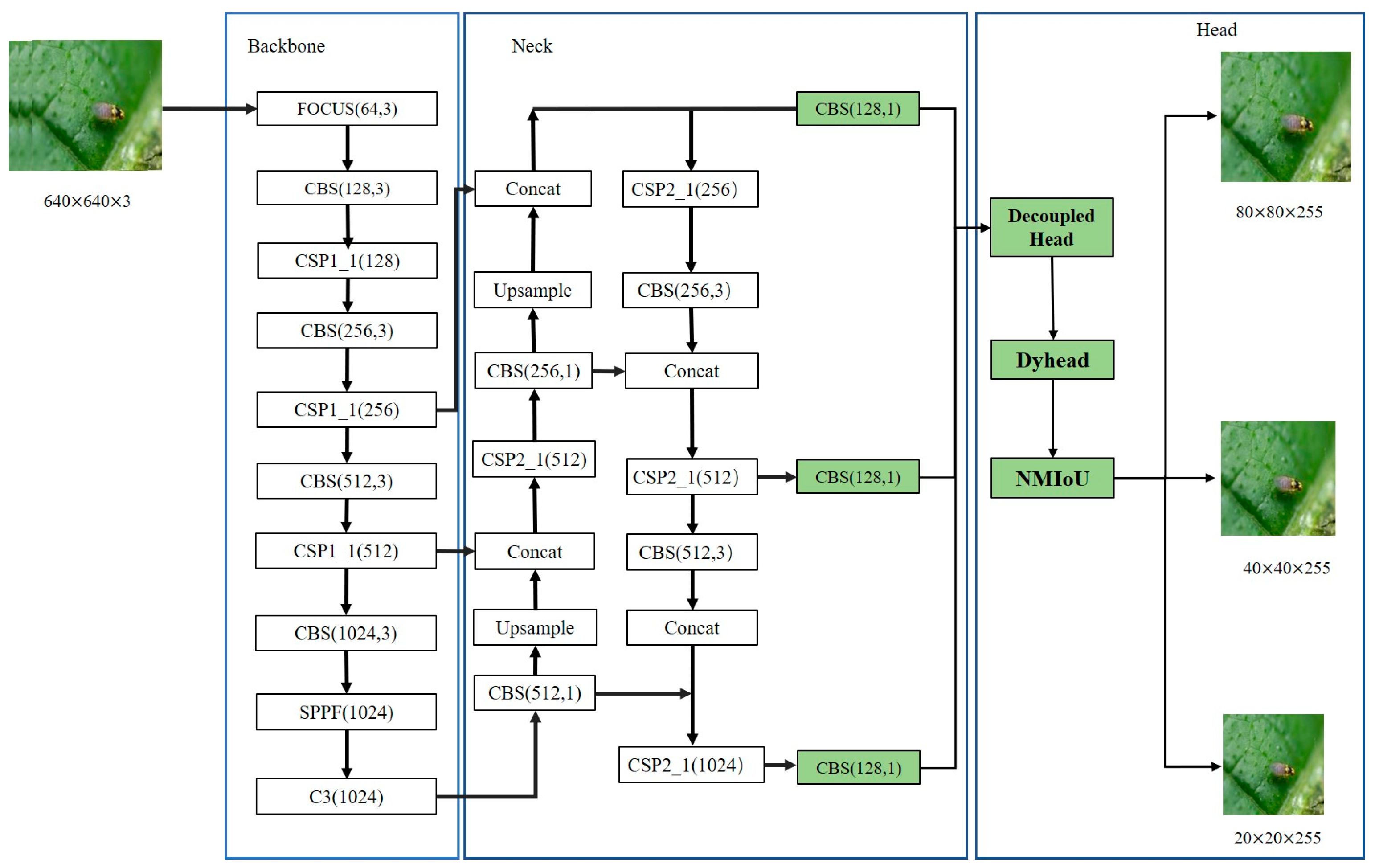
In this paper, a deep learning-based detection model, YOLONDD, is proposed, and its structure is shown in Figure 1.
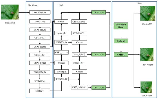
Figure 1.
Network structure diagram of YOLONDD, where the green rectangles are the improvement aspects of the model.
According to Figure 1, the main ideas of YOLONDD include three aspects: designing a new loss function NMIoU, adding a DyHead with an attention mechanism, and adding a decoupled head to Head.
Using the NWD [25] (Normalized Wasserstein Distance) metric in combination with MPDIoU [26] (Mean Pairwise Distance Intersection over Union), the NMIoU loss function is proposed, which can improve the sensitivity to the target frame and the small-scale detection ability, and the balance coefficient can be adjusted to achieve the weight of Loss.
DyHead is a target detection framework based on an attention mechanism. It can adaptively adjust the receptive field size to adapt to the scale change in different targets and improve the detection ability of targets at different scales. Meanwhile, DyHead utilizes a shared feature extraction network to reduce the number of computations and parameters.
The coupled head used in YOLOv5 has a simple design idea, which requires a large number of parameters and computational resources and is prone to overfitting. The decoupled head can extract the target location and category information separately, learn them through different network branches separately, and finally fuse them. It can effectively reduce the number of parameters and computational complexity and enhance the generalization ability and robustness of the model.
2.1.1. Designing a New Loss Function NMIoU
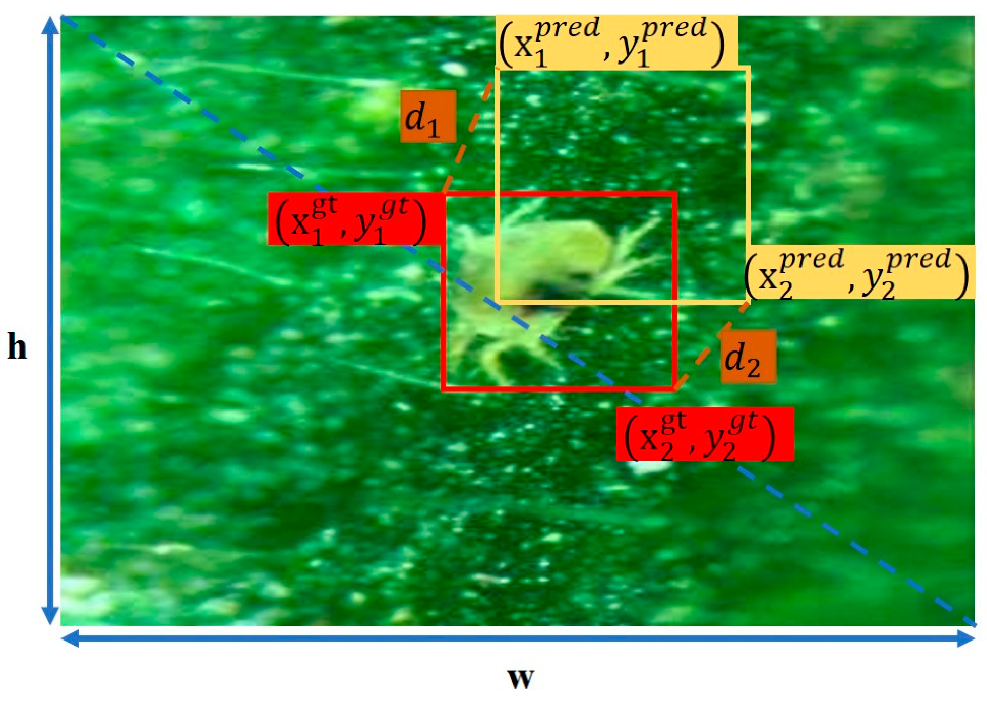
Small target detection is a very challenging problem in target detection in pest data where the pests are only a few pixels in size in the image. As the appearance information of small target pests is more difficult to detect, the current state-of-the-art detectors cannot get better results on small targets. We can also see from our experiments that loss functions such as IoU [27], CIoU [28], and DIoU are very sensitive to the positional deviation of small targets and greatly reduce the detection performance when they are used in anchor-based detectors. In order to solve this problem, we propose a loss function based on the combination of the NWD metric and the MPDIoU loss function-NMIoU, where the MPDIoU loss function is schematically shown in Figure 2.

Figure 2.
Schema of the MPDIoU loss function. Red rectangle means the ground truth and yellow one is the predicted result, where x and y represent the coordinates.
The loss function used in YOLOv5 is CIoU, which takes into account the distance between the target frame and the Anchor, the overlap, the scale, and the penalty term to make the target frame regression more stable. However, CIoU suffers from high computational complexity, does not take into account the case where the correct frame has the same aspect ratio as the predicted frame, is highly sensitive to the target frame, and is not applicable to large-scale differences.
The CIoU loss function cannot be optimized when the predicted box has the same aspect ratio as the actual labeled box, but the width and height values are completely different. MPDIoU can solve the above problem well; it is a comparative measure of bounding box similarity based on the distance of the minimum point, which takes into account all the relevant factors considered in the existing loss functions, such as the overlapping or non-overlapping area, the distance of the centroids, and the deviation of width and height. MPDIoU is determined by the four vertices of the bounding box in the upper left corner (, ), upper right corner (, ), lower left corner (, ), and lower right corner (, ). The general bounding box is determined by the center coordinates (, ) and the width and height . For this reason, we can calculate the four vertex coordinates as shown in the formula. The four vertex coordinates are obtained [29], and the distance between the two sets of vertices is calculated, and the minimum of these distances is chosen . Then, the ratio of the overlapping region of the predicted and real boxes to their concatenated region is calculated. The final MPDIoU loss function can be defined as Equation.
In Equation, , , , are the coordinates of the four vertices of the bounding box, is the coordinate of the center of the bounding box, is the width of the bounding box, and is the length of the bounding box.
The NWD metric is introduced to address the problem of high sensitivity to target boxes and its inapplicability to large-scale differences. The traditional IoU and its variants are discarded for the boxes with low confidence in the bounding box because, in these bounding boxes, the foreground and background pixels are concentrated on the center and the boundary of the bounding box, respectively, which leads to the low useful information in the box, and to this point, it affects the low confidence. NWD solves this problem well by assigning different weights to the pixels in the bounding box, with the center having the highest weight and decreasing from the center to the boundary. For this purpose, the bounding box is modeled as a two-dimensional Gaussian distribution, and then the distance of the distribution is calculated by the Wasserstein distance. The two-dimensional Gaussian distribution of the bounding box is defined by the centroid (,), width , and height . For the two-bounding box , Gaussian distributions, the Wasserstein distance can be obtained by calculating the difference between their means and covariances, and finally, the value domain of the Wasserstein distance is restricted to be between 0 and 1 by normalization, and the normalization factor is the maximum value of the two maximum values of the diagonal lengths of the bounding box.
In addition, NWD integration into YOLO is improved based on the label assignment, NMS, and regression loss function of IoU. In the NWD-based label assignment strategy, for training RPNs, positive labels will be assigned to two types of anchors: anchors with the highest NWD values and NWD values greater than and anchors with NWD values higher than the positive threshold for any real frame. Therefore, negative labels will be assigned to anchors if their NWD values are lower than the negative threshold for all real frames. In addition, anchors with neither positive nor negative labels assigned do not participate in the training process. where and are the original detectors. NMS is based on NWD. First, it sorts all the prediction frames based on their scores. The highest-scoring prediction frame M is selected, and all other prediction frames with significant overlap with M are suppressed. This process is recursively applied to the remaining boxes. Based on the regression loss of NWD, IoU-Loss is not able to provide gradients for the optimization network in some cases, and for this reason, the NWD metric is designed as a loss function:
As mentioned above, the NMIoU loss function is obtained by combining MPDIoU and NWD, and we just need to give reasonable balance coefficients to the NMIoU loss function to regulate the loss weights of MPDIoU and NWD. The formula for the NMIoU loss function is as follows:
In Equation, λ is the equilibrium coefficient that regulates the loss weights of MPDIoU and NWD.
2.1.2. Adding a DyHead with an Attention Mechanism
The detection head is a crucial component of the target detection model, whose role is to process the features of the last layer of the network and generate the results of target detection. In the target detection task, the detection head assumes several important roles. First, the detection head is responsible for target localization. The location information of the target frame is predicted through regression. Second, the detection head is also responsible for target classification. By predicting the category to which the target belongs through a classifier, the model is able to identify and label different objects in the image through the classification function of the detection head. In addition, the detection head is also responsible for generating the target score. The target score is used to measure the confidence or importance of each target in the detection results. This helps in filtering out the targets with high confidence levels, thereby improving the accuracy and reliability of the detection results. The role of the detection head in the target detection task is critical and indispensable. Through the functions of target localization, target classification, and target score generation, the detection head is able to achieve accurate localization and classification of targets in an image, providing important target detection results for real-world application scenarios.
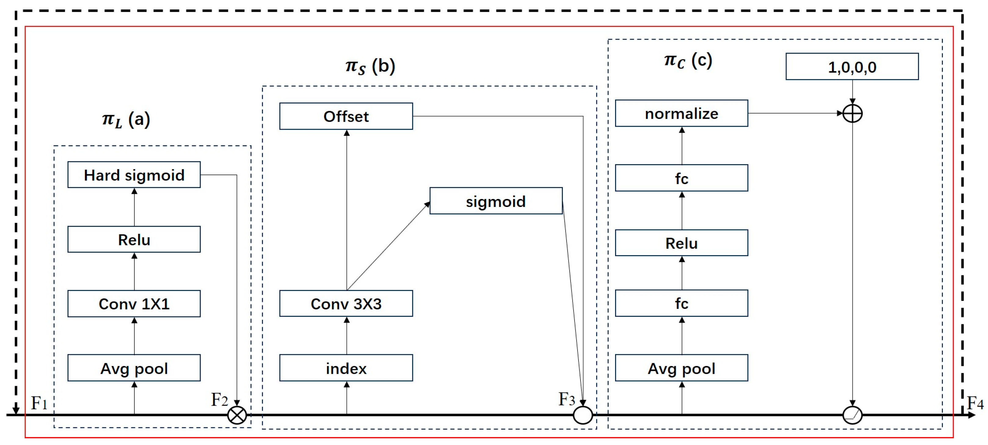
For this reason, this paper introduced the detection head DyHead in YOLOv5, which contains an attention mechanism. Dyhead consists of a scale-aware attention module, a spatial-aware attention module, and a task-aware attention module. When the scale-aware attention module processes the original feature map F1, it performs a global average pooling operation on the feature map, which aggregates features on different scales to obtain a multi-scale global representation. Subsequently, the above multi-scale feature maps are integrated using 1 × 1 convolution to fuse the features on different scales. Relu and Hard Sigmoid functions are used to enhance the nonlinear representation of the model for the multi-scale feature maps. Finally, the computed weights are multiplied with the original feature map to obtain the new feature map F2. When the Perceptual Attention module processes F2, the Index function extracts the positional information of the feature map, and subsequently, the extracted positional information is processed by a 3 × 3 deformable convolution and used to adjust the offsets of the convolution kernel, the sparse sampling, and the aggregation of the feature elements by the Sigmoid function. The offset function uses the obtained offsets to increase the weight share of the target shallow contour and edge information in the network. Finally, the acquired position information is appended to a new feature map F3. F3 is fed into the task-aware attention module, which reduces the spatial dimensionality of the feature map through an average pooling operation, followed by two fully connected layers to learn the inter-channel relationships. After the fully connected layers, the ReLU activation function is introduced to enhance the nonlinear representation of the features, and the scaling of the features is adjusted by a normalization operation. The normalization uses the scaling factor and offset factor in Batch Normalization for task-awareness, and the output of the task-aware attention module is used to obtain the desired feature map F4 through a composite operation, as shown in Figure 3.

Figure 3.
DyHead structure. (a) Scale-aware attention module. (b) Spatial-aware attention module. (c) Task-aware attention module.
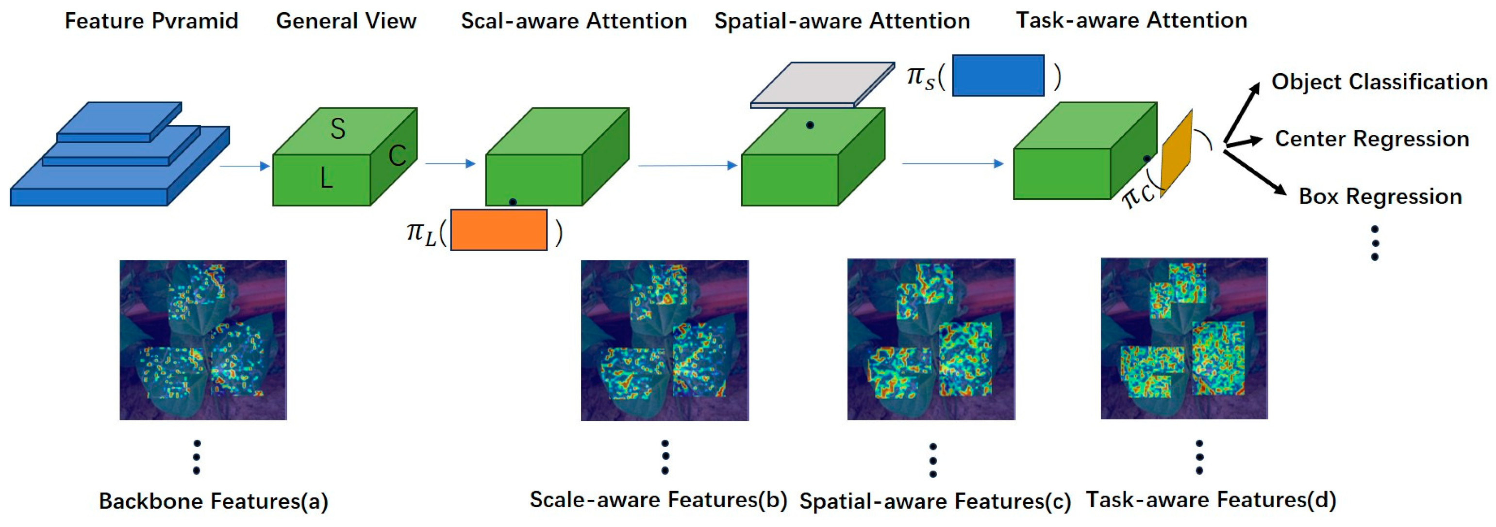
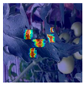
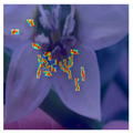
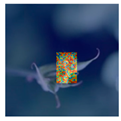
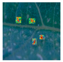
It uses the attention mechanism to unify the different target detection heads. As can be seen in Figure 4, the initial features are noisy due to domain differences, and for this reason, they cannot focus on the target well; firstly, after the original features are processed by the scale-aware attention module, the features become more sensitive to the targets at different scales; secondly, when the feature maps processed by the scale-aware attention module are processed by the spatial location-aware attention module, the features become more sparse, focusing on the foreground targets at different locations; Finally, after processing by the task-aware attention module, the features will form different activations based on different downstream tasks through the attention mechanism between feature levels for scale perception, between spatial locations for spatial perception, and within the output channel for task perception, as shown in Figure 4.
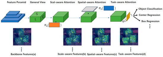
Figure 4.
DyHead image processing process. (a) Original feature map. (b) The scale-aware attention module processes the a-map. (c) The spatial-aware attention module processes the b-map as a feature map. (d) The task-aware attention module processes the c-map as a feature map. Where is a scale-aware attention module, is a spatial-aware attention module, and is a task-aware attention module. The feature map’s blue and cyan colors indicate regions with low detection values, while yellow, orange, and red indicate regions with higher detection values. They are in a progressive order.
In Equation, is the number of layers, is a linear function with 1 × 1 convolutional approximation, is the hard_sigmoid activation function, is the number of sparsely sampled positions, is the weight of the convolutional kernel, is the positional offset, is the spatial offset, is a self-learnable importance metric factor with respect to the position , is the slice of the feature tensor on a particular channel , and the weights obtained by network learning, and and are bias terms.
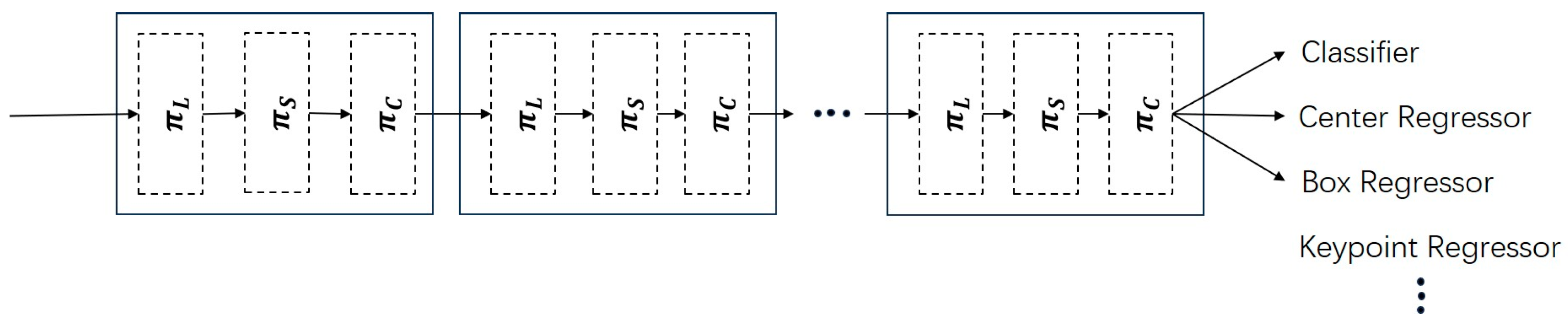
DyHead is introduced into YOLOv5, which is applied to a one-stage detector. The scale-aware attention module, the spatial location-aware attention module, and the task-aware attention module are combined as a group, and then the number of their cycles is selected for image processing, as shown in Figure 5.
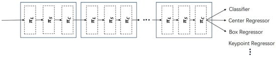
Figure 5.
DyHead applied a one-stage detector. is a scale-aware attention module, is a spatial-aware attention module, and is a task-aware attention module.
Normalization in DyHead uses the configuration of Group Normalization [30] (GN). GN aims to address the problem of performance degradation of Batch Normalization [31] (BN) on small batches of data or when the batch size varies, especially in non-convolutional layers of RNNs and CNNs. The core idea of GN is to perform normalization on each training batch to divide the channels in each feature map of the network into groups and normalize the channels within each group. Doing so reduces the model’s dependence on the batch size while maintaining the efficiency and effectiveness of the normalization operation. Specifically, the channels of the feature map are divided into G groups, each containing C/G channels. If the size of the feature map is [N, H, W, C], where N is the batch size, H and W are the height and width of the feature map, and C is the number of channels, then each group will contain C/G channels; the mean and variance are calculated for the channels within each group, and the channels in each group are normalized using these statistics. The normalization formula is as follows:
In Equation, is the input to the g layer of the network, is the mean of feature i for all samples in the current batch g, is the variance of feature for all samples in the current batch , and is a very small constant that prevents dividing by zero and ensures numerical stability. and are the learnable scaling and offsetting parameters.
The final normalized feature map is fed into the next layer of the network. It does this by calculating the mean and variance of all the samples in each batch and then using these statistics to normalize the inputs for the current batch. This results in a more stable distribution of inputs to the network and reduces the internal covariance bias, thus allowing the use of larger learning rates, faster training, and less sensitivity to initialization weights.
2.1.3. Adding Decoupled Head to Head
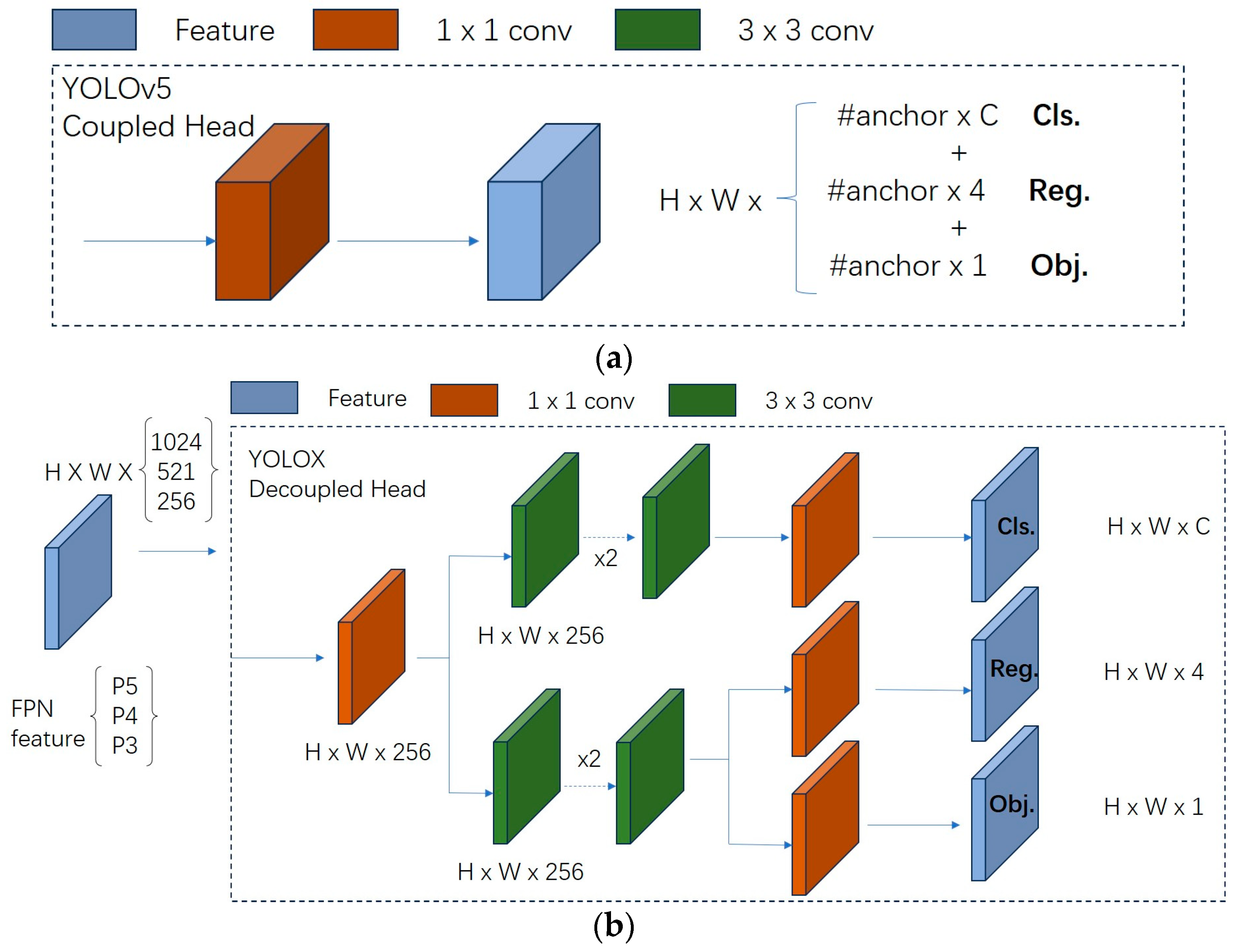
There is no decoupled head in YOLOv5, only a coupling header. The coupling head typically requires the feature map output from the convolutional layers to be fed directly into several fully connected or convolutional layers in order to generate outputs for the target locations and categories. Such a design brings a lot of parameters and computational resources to the model, and the model is also prone to overfitting. In contrast, a more efficient decoupled head structure is designed in YOLOv6 with the help of a hybrid channel strategy, which reduces the number of 3 × 3 convolutional layers in the decoupled head of YOLOX to only one. The width of the head is jointly scaled by the width multipliers of the Backbone and Neck. The delay is reduced while maintaining accuracy, mitigating the additional delay overhead associated with the 3 × 3 convolution in the decoupled head. This is shown in Figure 6.
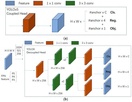
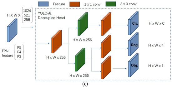
Figure 6.
Decoupled Head. (a) YOLOv5-coupled head. (b) YOLOX-decoupled head. (c) YOLOv6 decoupled head.
In this paper, with the help of YOLOv6’s decoupled head idea, the decoupled head is introduced for YOLOv5. The feature maps of P3, P4, and P5 in YOLOv5 are inputted, and the feature maps are processed by a 1 × 1 convolution and divided into two branches, and then the processed features are all processed by a 3 × 3 convolution, and the final output of the feature maps is processed by another 1 × 1 convolution, and the classification maps are obtained, respectively, a coordinate position map and a target frame confidence map.
2.2. Datasets
2.2.1. Data Acquisition and Preprocessing
The original 1426 images of the pest dataset used in the experiments in this paper were obtained from Kaggle [32]. Among them, the Leafminer flies were not included in the original dataset, which was collected by ourselves from the Internet, totaling 192 images. The Kaggle dataset was collected from inside the greenhouse, and in order to be closer to tomato leaf pests in the natural environment, we collected tomato leaf pests through the cultivation help grower website, where tomato pests were collected from tomato leaf pests photographed by the technicians in the natural environment, and we added the collected images to the public dataset. The tomato leaf pests on the website are all from the tomato leaf pests photographed by technicians in the natural environment, and we added the collected images to the public dataset, including 89 images of leafminer flies, 63 images of thrips, 68 images of tabacco budworm, and 510 images of spider leaf mite.
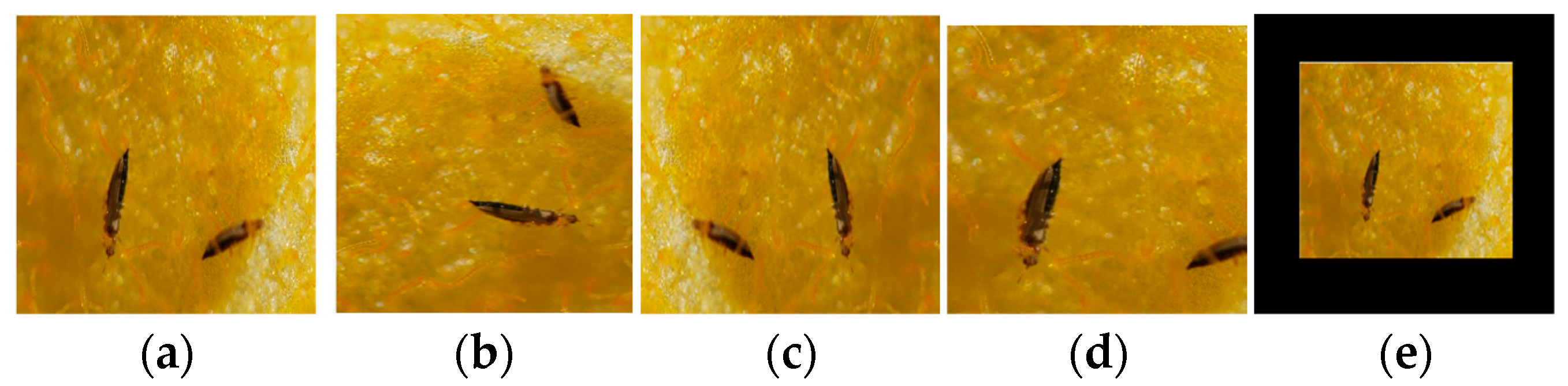
Secondly, data augmentation techniques such as rotation, mirroring, cropping, and scaling are used to increase the sample capacity and improve generalization. Some of the data are shown in Figure 7.
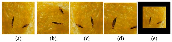
Figure 7.
Data augmentation. (a) Original image. (b) Rotation. (c) Mirroring. (d) Cropping. (e) Scaling.
Finally, the pest images in the dataset were labeled by the annotation software LabelImg 1.8.6 (EASY EAI, China) [33] to generate XML files. Although the YOLO series has provisions for dataset labeling files, the dataset was uniformly stored in PASCAL VOC8 [34] data format for better comparison experiments of various methods as well as experimental efficiency.
2.2.2. Pest Image Datasets
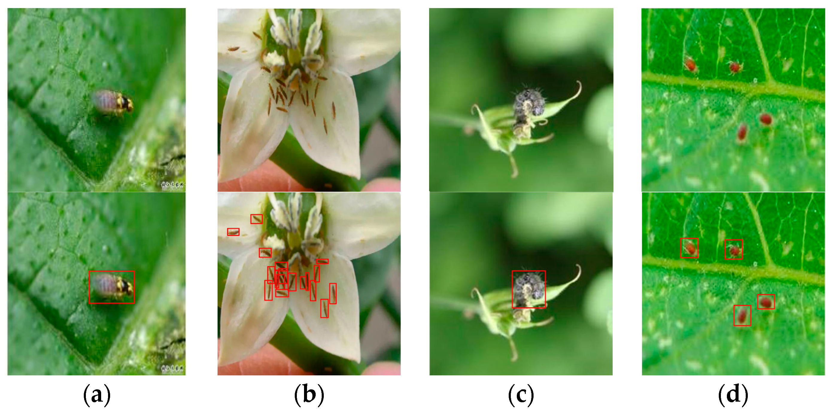
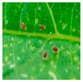
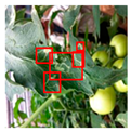
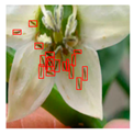
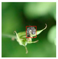
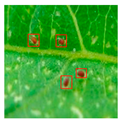
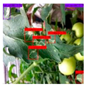
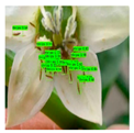
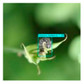
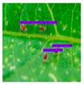
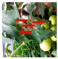
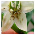
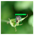
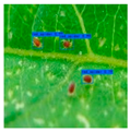
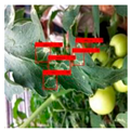
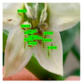
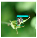
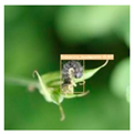
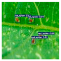
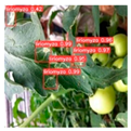
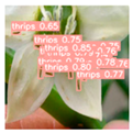
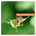
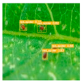
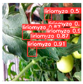
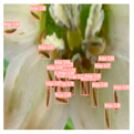
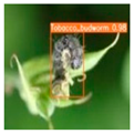
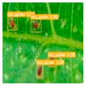
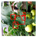
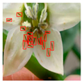
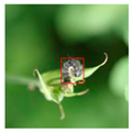
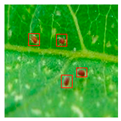
The images in this dataset were collected based on the pathological features, eggs, larvae, and adults caused by the pests on the leaves. Also, according to the type of pests in the images, the tomato pest images in this dataset are divided into leafminer flies, thrips, Tabacco Budworm, and spider leaf mite datasets, and the images are divided into a training set, a testing set, and a validation set according to 8:1:1, and some of the data are shown in Figure 8.

Figure 8.
Images of infested tomato leaves and their labels. (a) Leafminer flies. (b) Thrips. (c) Tabacco Budworm. (d) Spider leaf mite. Red boxes are labeled boxes.
Among them, 1426 images of pests containing 192, 180, 167, and 887 images of Leafminer flies, Thrips, Tabacco Budworm, and spider leaf mite tomato leaf pests, respectively. This dataset was expanded to 3479 images by image enhancement, as detailed in Table 1.

Table 1.
Size of pest datasets.
2.3. Experiment Scheme
This section carries out the experimental design in order to test the performance of the YOLONDD model proposed in this paper. Firstly, software and hardware equipment configuration is followed by dataset production and preprocessing required for this experiment, as well as the hyperparameter setting of the experimental network. Finally, the robustness test and ablation experiment.
2.3.1. Hardware and Software Configuration
In this paper, the PyTorch deep learning framework is used to train and test the network model, and the specific experimental configuration is shown in Table 2.
Table 2.
Experimental software and hardware configuration.
2.3.2. Determination of Training Parameters
The original YOLOv5 model, under the premise of the initial learning rate of 0.0001 and a Batch-size of 8, performed well on the PASCAL VOC2012 and COCO datasets. On this basis, according to the commonly used empirical values of network training hyperparameters, the hyperparameters of the YOLONDD network are finally determined after repeated tests, as shown in Table 3.
Table 3.
The optimized hyperparameters.
2.3.3. Comparison Experiments
- (1)
- In order to determine the base loss function of this paper, a variety of different loss functions were added to the tomato leaf pest images for comparison experiments, and AP was selected as an index to test the detection performance of this paper’s Model.
- (2)
- In order to determine the equilibrium coefficient between NWD and MPDIoU, values are taken in the interval [0, 1], comparison experiments are conducted, and AP is selected as an indicator to test the detection performance of the model in this paper.
- (3)
- In order to test the normalization functions GN and BN in DyHead as well as the number of cycles of DyHead on the tomato leaf pest images, comparative experiments were conducted, and AP and training time were selected as indicators to test the detection performance of the model in this paper.
- (4)
- In order to test the performance of the model YOLONDD proposed in this paper in the tomato pest image detection task, comparative experiments are conducted with YOLONDD with traditional target detection models such as Faster R-CNN [35], SSD [36], YOLOv7 [37], RetinaNet, YOLOv5, and YOLOv8. The experiment divides the total dataset into a training set, testing set, and validation set according to the ratio of 80%, 10%, and 10%, which are used to train the model and conduct the test, and selects AP and F1 as the indexes to test the detection performance of this paper’s model, and FPS, training time, and single-image prediction time are selected as the indexes to verify the detection efficiency of the YOLONDD proposed in this paper.
In addition, detection comparison experiments are conducted on the constructed tomato pest dataset to test the generalization ability of the model and verify the robustness of YOLONDD proposed in this paper.
2.3.4. Ablation Experiments
To verify the effectiveness of the designed new loss function MNIoU, the introduction of the detection head DyHead with an attention mechanism, and the introduction of the decoupled head, seven sets of ablation experiments are performed on the total dataset.
- (1)
- YOLON: On the basis of the original YOLOv5 network, the original loss function CIOU is replaced by the loss function NMIOU designed in this paper.
- (2)
- YOLOD1: On the basis of the original YOLOv5 network, introducing the DyHead.
- (3)
- YOLOD2: On the basis of the original YOLOv5 network, adding a decoupled head.
- (4)
- YOLOND1: On the basis of YOLON, the DyHead detection head is introduced into the network model.
- (5)
- YOLOND2: On the basis of YOLON, a decoupled head is introduced in the network model.
- (6)
- YOLOD1D2: On the basis of YOLOD1, a decoupled head is introduced in the network model.
- (7)
- YOLONDD: Based on YOLOND1, a decoupled head is introduced in the network model, which is the method proposed in this paper.
2.4. Evaluation Indicators
In this paper, Average Precision (AP), Frames Per Second (FPS), and F1 score (F1) are used as important evaluation metrics for the detection of tomato leaf pests to analyze the network detection performance.
- (1)
- Average Precision (AP)
AP is the area enclosed by the PR curve and the coordinate axis, and is calculated as follows:
In Equation, is the number of predicted bounding boxes that are correctly categorized and have the correct coordinates of the bounding box, is the number of predicted bounding boxes that are incorrectly categorized, is the number of bounding boxes that are not predicted, () is the precision rate, and () is the recall rate.
- (2)
- Frames Per Second (FPS)
FPS is the number of frames per second transmitted, which indicates the number of images that can be processed in a second or the time it takes to process an image to evaluate the detection speed, the shorter the time, the faster the speed. The calculation formula is as follows:
- (3)
- F1 score (F1)
The F1 score is a kind of reconciled average of model precision and recall, calculated as follows:
3. Results
3.1. Loss Function Analysis
In order to explore the advantages and disadvantages of different loss functions in detecting the dataset, this paper conducts controlled experiments on CIoU, EIoU, DIoU, GIoU, WIoU, SIoU, and MPDIoU to select the optimal loss function. The results are shown in Table 4.
Table 4.
Comparison of different loss functions.
As can be seen from Table 4, MPDIoU is 2.52%, 1.71%, 0.56%, 0.22%, and 0.45% higher than CIoU, EIoU, DIoU, GoU, and SIoU. Therefore, MPDIoU is adopted as our base loss function.
3.2. NMIoU Balance Coefficient Analysis
In order to explore the advantages and disadvantages of different Losses of NDW and Losses of MPDIoU-specific gravity for the detection of the dataset, we conducted controlled experiments on different Loss-specific gravity to select the optimal Loss-specific gravity. The results are shown in Table 5.
Table 5.
Comparison of the NMIoU balance factor.
From Table 5, it can be seen that when the balance coefficient λ of MPDIoU and NWD in YOLOv5 is 0.6, NMIoU is higher than the others. Therefore, λ = 0.6 is used as the balance coefficient of the loss function NMIoU.
3.3. Comparison of DyHead Normalization Functions GN and BN
In order to explore the advantages and disadvantages of different DyHead normalization functions for the detection of the dataset, this paper added the BN normalization function, and conducted controlled experiments on GN and BN to select the optimal normalization function and the number of cycles. The results are shown in Table 6.
Table 6.
Comparison of DyHead normalization functions GN and BN.
As can be seen from Table 6, DyHead achieves better results in the tomato leaf pest dataset when DyHead in YOLOv5 uses the GN normalization function and achieves an accuracy of 88.90% at a cycle time of 2, which is higher compared with YOLOv5, GN4, GN6, BN2, BN4, and BN6. GN2 has a time of 3.693 h, which is improved relative to the others. Relative to YOLOv5 itself, YOLOv5 uses a DyHead detection head, which needs to be processed cyclically through the scale-aware attention module, the spatial location-aware attention module, and the task-aware attention module, resulting in an increase in time, which is an unavoidable time increase. Relative to the short training time of BN = 2, the difference of the main normalization module GN needs to group the channels when calculating the mean and variance, which will introduce some additional computational overhead. Furthermore, GN introduces the concept of groups, which will increase the total number of parameters of the model, thus affecting the training speed. However, from Table 6, it can be seen that the mAP of GN = 2 has the highest accuracy. Therefore, the GN normalization function is adopted and looped twice as the optimal parameter pairing for DyHead.
3.4. Detection Performance of the YOLONDD Model
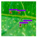
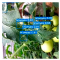
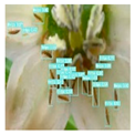
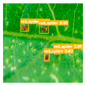
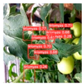
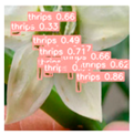
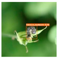
The detection results of YOLONDD and other models are shown in Table 7, and the thermal effects of them are shown in Table 8.
Table 7.
Effect of detection using different models.
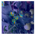
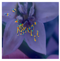
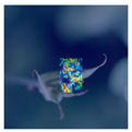
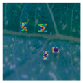
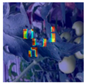
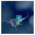
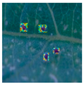
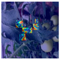
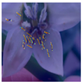
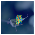
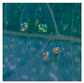
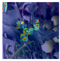
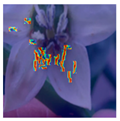
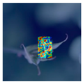
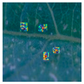
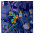
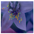
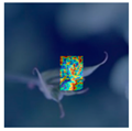
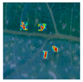
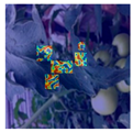
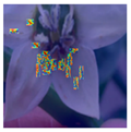
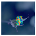
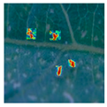
Table 8.
Thermal effects of different models. The red box is the labeled box. The blue and cyan colors in the detection box indicate areas with low detection values, and the yellow, orange, and red colors indicate areas with high detection values. Their order is progressive.
From Table 7, it can be seen that YOLONDD has a higher detection accuracy for tomato leaf pests compared with the other six models, and there is less leakage of pests for small targets.
From Table 8, it can be seen that YOLONDD performs better in tomato leaf pests compared with the other six models, and the red and yellow high-value areas are more concentrated.
The performance of tomato leaf pest image detection using YOLONDD and the other six models was compared using mAP, FPS, training time, F1, and single image prediction time as metrics, and the results are shown in Table 9, Table 10 and Table 11.
Table 9.
mAP of different models for tomato leaf pest detection.
Table 10.
Efficiency of different models for tomato leaf pest detection.
Table 11.
F1 scores of different models for tomato leaf pest detection.
As can be seen from the table, the mAP of YOLONDD is 16.14%, 16.25%, 3.33%, 9.41%, 0.56%, and 12.48% higher than SSD, Faster R-CNN, YOLOv5, RetinaNet, YOLOv7, and YOLOv8, respectively. The experimental data proves that the proposed NMIoU loss function improves target frame sensitivity and small-scale detection ability.
From the table, we can see that the training time of YOLONDD is 3.347 h, which is faster than the other models. The single-image prediction time of YOLONDD is 18.90 ms, which is the fastest. The FPS of YOLONDD with Batch size = 1 is 52.91 ms, which is faster than Faster R-CNN, RetinaNet, and YOLOv7. YOLOv8 is faster than this model because it uses a more efficient architecture, a better feature extractor, and a more effective neck and head structure to improve training efficiency. SSD uses a more lightweight network structure, and SSD performs target detection on multiple scales of feature maps, which allows the model to capture targets at different resolutions and will improve the efficiency of training.
Compared with the YOLOv5 model, the training time of YOLONDD is 59.53%, and the single-image prediction time is increased by 7.1 ms, which is due to the fact that the YOLOv5 model itself has a simpler model structure and a smaller number of parameters, which reduces the model training time as well as the single-image prediction time. The slow training speed of YOLONDD is due to the use of the DyHead detection head, which extracts the feature maps several times for optimization, thus reducing the training speed. However, it can be seen from Table 7, Table 8 and Table 9 that its detection accuracy is not as good as that of the present model, YOLONDD. Overall, in the present model, by replacing the loss function NMIoU with CIoU, adding the detection head with the attention mechanism DyHead as well, and changing the coupling head of YOLOv5 to a decoupled head, the detection time is increased compared with the YOLOv5 model, but the model detection accuracy is also improved.
As can be seen from the table, the mF1 of YOLONDD is 88.60%, which is faster than the other models. Especially in Leafminer flies, there is an 8.88% improvement relative to the original YOLOv5. It shows that the YOLONDD can extract the features of pests well and improve the detection ability of images.
3.5. Results of Ablation Experiments
Ablation experiments were carried out based on the ablation experiment scheme described in Section 2.3.4. The results of the experiments are shown in Table 12.
Table 12.
Performance of different ablation methods.
From the results of the ablation experiments in Table 12, it can be seen that the mean average precision (mAP) of YOLON, YOLOD1, and YOLOD2, when paired individually, are all improved compared with that of YOLOv5, which illustrates the fact that the replacement of the loss function CIoU by the loss function NMIoU, the introduction of the detection head with an attentional mechanism, DyHead, and the introduction of a decoupled head, can improve the model’s detection precision to some extent.
It can be seen that the accuracy decreases relative to YOLON, YOLOD1, and YOLOD2, indicating that DyHead and decoupled heads have different focuses in feature extraction and representation. When they are combined, feature incoherence occurs, resulting in a model that does not effectively utilize all the useful information. The loss function NMIoU is combined with DyHead, while the NMIoU loss function focuses on optimizing the positioning accuracy of the bounding box.
Combining the three, it can be seen that the accuracy is at its highest, and the decoupled head processes the feature maps of P3, P4, and P5 in batches, which can result in classification maps, coordinate position maps, and target box confidence maps. Whereas DyHead enhances the feature representation through the attention mechanism, the NMIoU loss function focuses on optimizing the positioning accuracy of the bounding box. The decoupled head can just bring out the focused advantages of DyHead and NMIoU.
The training detection efficiency of each ablation experiment model was also compared, and the results are shown in Table 13.
Table 13.
Efficiency of different ablation methods.
As can be seen from Table 13, the training time and prediction time of the YOLON, YOLOD1, and YOLOD2 models increased relative to the traditional YOLOv5, indicating that the inclusion of the detection head DyHead with attention mechanism, loss function, and the introduction of the decoupled head alone increase the computational complexity of the model, which in turn increases the training time of the model. With YOLOD1, the training time of the model is reduced by adding the decoupled head and NMIoU separately. Because YOLOv5 adopts the structure of a coupled head, adding DyHead for this purpose will increase the complexity of the model, and DyHead will perform cyclic feature extraction on the image twice, which will enhance the number of parameters in the model even more and increase the training time. However, the decoupled head will process the feature maps of P3, P4, and P5 in batches, which will save a lot of time. Adding the NMIoU loss function can simplify the process of calculating the target position, and the structure of NMIoU can improve the convergence speed. Therefore, adding a decoupled head and NMIoU loss function can relatively reduce the training time of the model.
4. Discussion
In traditional pest management, the identification of pests relies on the farmers’ empirical judgment, which is the disadvantage of the approach that could be more efficient and more balanced on subjective judgment. According to the characteristics of pests in natural environments, factors such as the occlusion of pests, complex backgrounds, colors, and target size can affect the model’s effectiveness for detection and identification. Therefore, there are challenges in detecting small target pests accurately and quickly. Currently, there are several studies on crop pest detection and recognition, but there are fewer studies on small-target crop pests. Hu et al. [38] improved YOLOv5 for tomato pest detection, and the model’s mAP could reach 98.10%. Still, because the authors’ dataset was annotated with the entire diseased leaf, they could not verify that the model performed well in complex scenarios and with small targets. Wang et al. [39] improved YOLOv3 for early detection of tomato pests and diseases in complex backgrounds, and the model achieved better detection results, but the model has leakage in small targets. Although all these studies have excellent performance in pest and disease detection, they need more research on small targets with complex backgrounds. For this reason, this paper proposes a method for pest detection of small targets in complex contexts. The validation results on the self-constructed dataset show that YOLONDD is better than other models in detecting small targets under complex backgrounds, which can effectively detect pests and improve the accuracy of pest detection.
Although YOLONDD has a mAP of 90.1% in the dataset, which can satisfy the current detection task, there is still a leakage of detection, indicating that there is still room for improvement in the model’s ability to detect small-target pests in complex backgrounds. Combined with the heat map, it can be seen that YOLONDD pays attention to the areas where pests or pest infestation parts exist, which indicates that some pests or pest infestation parts cannot be detected. The main reason for this may be that although the newly designed NMIou loss function reduces some of the missed detections due to leaf occlusion, some of the frames with low scores are still filtered when the vertex coordinates are calculated for the overlapping frames, which is a problem that needs to be paid attention to in the future.
Currently, some tomato leaf pests are used as research objects in this paper, but many pests still have practical applications, and more pest datasets are needed to improve the model’s applicability. The pest collection method must also be further standardized, considering factors such as shading and light conditions to enhance the model’s generalization ability.
5. Conclusions
Fast and accurate identification of tomato pests can help tomato farmers detect pests in their tomato crops and improve tomato yields, as well as agro-horticultural to improve plant health and visual perception, and can help specialist experts easily determine the type of pests.
A network target detection model based on deep learning, YOLONDD, was proposed in this paper. A new loss function NMIoU is designed in the model to improve the ability of anomaly processing, improve the model’s ability to detect and recognize objects at different scales, and improve the robustness to scale changes; the detection head DyHead containing an attention mechanism is introduced to improve the ability to detect targets at different scales. Adding a DyHead with an attention mechanism improves the detection ability of targets at different scales, reduces the number of computations and parameters, improves the accuracy of target detection, improves the overall performance of the model, and accelerates the training process. Adding a decoupled head to Head can effectively reduce the number of parameters and the computational complexity, and enhance the model’s generalization ability and robustness.
The model proposed in this paper, YOLONDD, was shown to detect tomato leaf pests more effectively in images than other test models. The mAP of the whole dataset of tomato pest images reached 90.1%. All of these are better than the target detection models such as Faster R-CNN, SSD, YOLOv5, RetinaNet, YOLOv7, YOLOv8, etc., and realize more efficient and accurate detection on tomato leaf pest images.
In this paper, we achieved a more accurate detection effect on the results of pest images, but there are still some issues to face. The future directions of related research include the following aspects: how to detect and eliminate the shades in the tomato leaf images; how to accurately detect pests if the colors of pests and leaves are similar; and how to recognize pests if there are some obstacles on parts of pests, such as other leaves or stalks, so as to reduce the influence of shadows, colors, and occlusions on the detection of tomato pests in complex backgrounds of real environments.
Author Contributions
Conceptualization, R.X. and G.W.; methodology, R.X., G.W., F.Y., L.M., P.W. and X.Y.; software, R.X.; validation, R.X.; formal analysis, R.X., P.W. and X.Y.; investigation, R.X., G.W., F.Y., L.M., P.W. and X.Y.; data curation, R.X.; writing—original draft. R.X.; resources, G.W., F.Y. and L.M.; writing—review and editing, G.W.; funding acquisition, L.M. and P.W. All authors have read and agreed to the published version of the manuscript.
Funding
This study was supported by the Key Research and Development Program of Zhejiang Province (Grant number: 2021C02005) and Zhejiang Provincial Commonweal Projects (Grant number: LGG21F020001).
Data Availability Statement
The code for our proposed model YOLONDD and dataset used in the experiments can be found on GitHub: https://github.com/zafucslab/YOLONDD (accessed on 6 May 2024).
Conflicts of Interest
The authors declare no conflicts of interests.
References
- Crispi, G.M.; Valente, D.S.M.; de Queiroz, D.M.; Momin, A.; Fernandes-Filho, E.I.; Picanço, M.C. Using Deep Neural Networks to Evaluate Leafminer Fly Attacks on Tomato Plants. Agriengineering 2023, 5, 273–286. [Google Scholar] [CrossRef]
- Xu, Y.; Gao, Z.; Zhai, Y.; Wang, Q.; Gao, Z.; Xu, Z.; Zhou, Y. A CNNA-Based Lightweight Multi-Scale Tomato Pest and Disease Classification Method. Sustainability 2023, 15, 8813. [Google Scholar] [CrossRef]
- Asiry, K.A.; Huda, M.N.; Mousa, M.A.A. Abundance and Population Dynamics of the Key Insect Pests and Agronomic Traits of Tomato (Solanum lycopersicon L.) Varieties under Different Planting Densities as a Sustainable Pest Control Method. Horticulturae 2022, 8, 976. [Google Scholar] [CrossRef]
- Zeng, X.; Huang, C.; Zhan, L. Image recognition method of agricultural pests based on multisensor image fusion technology. Adv. Multimed. 2022, 2022, 6359130. [Google Scholar] [CrossRef]
- Harris, C.G.; Andika, I.P.; Trisyono, Y.A. A Comparison of HOG-SVM and SIFT-SVM Techniques for Identifying Brown Planthoppers in Rice Fields. In Proceedings of the 2022 IEEE 2nd Conference on Information Technology and Data Science (CITDS), Debrecen, Hungary, 16–18 May 2022; pp. 107–112. [Google Scholar]
- Kasinathan, T.; Singaraju, D.; Uyyala, S.R. Insect classification and detection in field crops using modern machine learning techniques. Inf. Process. Agric. 2021, 8, 446–457. [Google Scholar] [CrossRef]
- Zhang, W.; Huang, H. AgriPest-YOLO: A rapid light-trap agricultural pest detection method based on deep learning. Front. Plant Sci. 2022, 13, 1079384. [Google Scholar] [CrossRef] [PubMed]
- Türkoğlu, M.; Hanbay, D. Plant disease and pest detection using deep learning-based features. Turk. J. Electr. Eng. Comput. Sci. 2019, 27, 1636–1651. [Google Scholar] [CrossRef]
- Kuzuhara, H.; Takimoto, H.; Sato, Y.; Kanagawa, A. Insect pest detection and identification method based on deep learning for realizing a pest control system. In Proceedings of the 2020 59th Annual Conference of the Society of Instrument and Control Engineers of Japan (SICE), Chiang Mai, Thailand, 23–26 September 2020; pp. 709–714. [Google Scholar]
- Venkatasaichandrakanth, P.; Iyapparaja, M. Pest Detection and Classification in Peanut Crops Using CNN, MFO, and EViTA Algorithms. IEEE Access 2023, 11, 54045–54057. [Google Scholar] [CrossRef]
- Pattnaik, G.; Parvathi, K. Automatic detection and classification of tomato pests using support vector machine based on HOG and LBP feature extraction technique. In Progress in Advanced Computing and Intelligent Engineering: Proceedings of ICACIE 2019; Springer: Singapore, 2021; Volume 2, pp. 49–55. [Google Scholar]
- Cortes, C.; Vapnik, V. Support-vector networks. Mach. Learn. 1995, 20, 273–297. [Google Scholar] [CrossRef]
- Liang, W.; Kirk, K.R.; Greene, J.K. Estimation of soybean leaf area, edge, and defoliation using color image analysis. Comput. Electron. Agric. 2018, 150, 41–51. [Google Scholar] [CrossRef]
- da Silva Vieira, G.; Rocha, B.M.; Fonseca, A.U.; de Sousa, N.M.; Ferreira, J.C.; Cabacinha, C.D.; Soares, F. Automatic detection of insect predation through the segmentation of damaged leaves. Smart Agric. Technol. 2022, 2, 100056. [Google Scholar] [CrossRef]
- Fang, W.; Guan, F.; Yu, H.; Bi, C.; Guo, Y.; Cui, Y.; Su, L.; Zhang, Z.; Xie, J. Identification of wormholes in soybean leaves based on multi-feature structure and attention mechanism. J. Plant Dis. Prot. 2023, 130, 401–412. [Google Scholar] [CrossRef]
- Zhu, R.; Hao, F.; Ma, D. Research on Polygon Pest-Infected Leaf Region Detection Based on YOLOv8. Agriculture 2023, 13, 2253. [Google Scholar] [CrossRef]
- Zhu, L.; Li, X.; Sun, H.; Han, Y. Research on CBF-YOLO detection model for common soybean pests in complex environment. Comput. Electron. Agric. 2024, 216, 108515. [Google Scholar] [CrossRef]
- Ye, R.; Gao, Q.; Qian, Y.; Sun, J.; Li, T. Improved YOLOv8 and SAHI Model for the Collaborative Detection of Small Targets at the Micro Scale: A Case Study of Pest Detection in Tea. Agronomy 2024, 14, 1034. [Google Scholar] [CrossRef]
- Tian, Y.; Wang, S.; Li, E.; Yang, G.; Liang, Z.; Tan, M. MD-YOLO: Multi-scale Dense YOLO for small target pest detection. Comput. Electron. Agric. 2023, 213, 108233. [Google Scholar] [CrossRef]
- Lippi, M.; Bonucci, N.; Carpio, R.F.; Contarini, M.; Speranza, S.; Gasparri, A. A yolo-based pest detection system for precision agriculture. In Proceedings of the 2021 29th Mediterranean Conference on Control and Automation (MED), Puglia, Italy, 22–25 June 2021; pp. 342–347. [Google Scholar]
- Mamdouh, N.; Khattab, A. YOLO-based deep learning framework for olive fruit fly detection and counting. IEEE Access 2021, 9, 84252–84262. [Google Scholar] [CrossRef]
- Yang, S.; Xing, Z.; Wang, H.; Dong, X.; Gao, X.; Liu, Z.; Zhang, X.; Li, S.; Zhao, Y. Maize-YOLO: A new high-precision and real-time method for maize pest detection. Insects 2023, 14, 278. [Google Scholar] [CrossRef] [PubMed]
- Dai, X.; Chen, Y.; Xiao, B.; Chen, D.; Liu, M.; Yuan, L.; Zhang, L. Dynamic head: Unifying object detection heads with attentions. In Proceedings of the IEEE/CVF Conference on Computer Vision and Pattern Recognition, Virtual, 19–25 June 2021; pp. 7373–7382. [Google Scholar]
- Li, C.; Li, L.; Jiang, H.; Weng, K.; Geng, Y.; Li, L.; Ke, Z.; Li, Q.; Cheng, M.; Nie, W.; et al. YOLOv6: A single-stage object detection framework for industrial applications. arXiv 2022, arXiv:2209.02976. [Google Scholar]
- Wang, J.; Xu, C.; Yang, W.; Yu, L. A normalized Gaussian Wasserstein distance for tiny object detection. arXiv 2021, arXiv:2110.13389. [Google Scholar]
- Siliang, M.; Yong, X. Mpdiou: A loss for efficient and accurate bounding box regression. arXiv 2023, arXiv:2307.07662. [Google Scholar]
- Jiang, B.; Luo, R.; Mao, J.; Xiao, T.; Jiang, Y. Acquisition of localization confidence for accurate object detection. In Proceedings of the European Conference on Computer Vision (ECCV), Munich, Germany, 8–14 September 2018; pp. 784–799. [Google Scholar]
- Zheng, Z.; Wang, P.; Liu, W.; Li, J.; Ye, R.; Ren, D. Distance-IoU loss: Faster and better learning for bounding box regression. Proc. AAAI Conf. Artif. Intell. 2020, 34, 12993–13000. [Google Scholar] [CrossRef]
- Mo, L.; Shi, L.; Wang, G.; Yi, X.; Wu, P.; Wu, X. MISF: A Method for Measurement of Standing Tree Size via Multi-Vision Image Segmentation and Coordinate Fusion. Forests 2023, 14, 1054. [Google Scholar] [CrossRef]
- Wu, Y.; He, K. Group normalization. In Proceedings of the European Conference on Computer Vision (ECCV), Munich, Germany, 8–14 September 2018; pp. 3–19. [Google Scholar]
- Ioffe, S.; Szegedy, C. Batch normalization: Accelerating deep network training by reducing internal covariate shift. In Proceedings of the International Conference on Machine Learning, Lille, France, 7–9 July 2015; pp. 448–456. [Google Scholar]
- Available online: https://www.kaggle.com/datasets/kaustubhb999/tomatoleaf (accessed on 21 June 2022).
- Available online: https://github.com/HumanSignal/labelImg (accessed on 1 July 2022).
- Li, Q.; Xie, B.; You, J.; Bian, W.; Tao, D. Correlated logistic model with elastic net regularization for multilabel image classification. IEEE Trans. Image Process. 2016, 25, 3801–3813. [Google Scholar] [CrossRef] [PubMed]
- Ren, S.; He, K.; Girshick, R.; Sun, J. Faster R-CNN: Towards real-time object detection with region proposal networks. Adv. Neural Inf. Process. Syst. 2015, 28. [Google Scholar] [CrossRef]
- Liu, W.; Anguelov, D.; Erhan, D.; Szegedy, C.; Reed, S.; Fu, C.Y.; Berg, A.C. Ssd: Single shot multibox detector. In Proceedings of the Computer Vision–ECCV 2016: 14th European Conference, Amsterdam, The Netherlands, 11–14 October 2016; Proceedings, Part I 14. Springer International Publishing: Berlin/Heidelberg, Germany, 2016; pp. 21–37. [Google Scholar]
- Wang, C.Y.; Bochkovskiy, A.; Liao HY, M. YOLOv7: Trainable bag-of-freebies sets new state-of-the-art for real-time object detectors. In Proceedings of the IEEE/CVF Conference on Computer Vision and Pattern Recognition, Vancouver, BC, Canada, 24 June 2023; pp. 7464–7475. [Google Scholar]
- Hu, W.; Hong, W.; Wang, H.; Liu, M.; Liu, S. A Study on Tomato Disease and Pest Detection Method. Appl. Sci. 2023, 13, 10063. [Google Scholar] [CrossRef]
- Wang, X.; Liu, J.; Zhu, X. Early real-time detection algorithm of tomato diseases and pests in the natural environment. Plant Methods 2021, 17, 43. [Google Scholar] [CrossRef]


Disclaimer/Publisher’s Note: The statements, opinions and data contained in all publications are solely those of the individual author(s) and contributor(s) and not of MDPI and/or the editor(s). MDPI and/or the editor(s) disclaim responsibility for any injury to people or property resulting from any ideas, methods, instructions or products referred to in the content. |
© 2024 by the authors. Licensee MDPI, Basel, Switzerland. This article is an open access article distributed under the terms and conditions of the Creative Commons Attribution (CC BY) license (https://creativecommons.org/licenses/by/4.0/).