Abstract
Mushroom cap is a key trait in the growth process and its phenotypic parameters are essential for automatic cultivation and smart breeding. However, the edible mushrooms are usually grown densely with mutual occlusion, which is difficult to obtain the phenotypic parameters non-destructively. Although deep learning methods achieve impressive performance with superior generalization capabilities, they require a large amount of ground truth label of the occluded target, which is a challenging task due to the substantial workload. To overcome this obstacle, a novel synthetic cap occlusion image method was proposed for rapidly generating edible mushroom occlusion datasets using raw images, in which the ground truth is obtained from the real world and the occlusion is randomly generated for simulating real scenes. Moreover, variants of amodal instance segmentation models with different backbone were trained and evaluated on our synthetic occlusion image datasets. Finally, an amodal mask-based size estimation method was presented to calculate the width and length of the cap. The experimental results showed that the amodal instance segmentation achieved an AP@[0.5:0.95] of 82%, 93% and 96% on Oudemansiella raphanipes, Agrocybe cylindraceas and Pholiota nameko synthetic cap datasets, respectively, with a size of 1024 × 1024 px, which indicates that our occlusion image synthesis method can effectively simulate the real cap occlusion situation. The size estimation method achieved an of 0.95 and 0.98 between predictive amodal caps and manually labeled caps for the length and width of Agrocybe cylindraceas cap, respectively, which can be applied to obtain the phenotypic parameters of each cap effectively and accurately. These methods not only meet the demand for automatic monitoring of edible mushroom morphology in factories but also provide technical support for intelligent breeding.
1. Introduction
The edible mushroom is rich in vitamins and minerals, which provide the human body with required nutrients. With the increased awareness of edible mushrooms, they are becoming increasingly popular [1,2]. The morphological characteristics of the mushroom cap are one of the key features in their cultivation. The changes in its size and morphology not only allow farmers to understand its growth status but also provide breeders with evidence for the breeding process. Furthermore, it is also an important indicator of the physiology, genetics and evolution of edible mushrooms, and it is essential to improve the yield of mushroom and mycology research. Unfortunately, traditional cap parameter measurement of edible mushrooms relies on manual measuring, which is subjective, repetitive and time-consuming [3]. Therefore, it is necessary to develop a non-destructive and rapid approach for obtaining the morphological parameters of edible mushroom caps.
With the rapid development of computer vision technology, image-based research has applied to non-contact, non-destructive, high-throughput acquisition of acquiring plants’ morphological parameters. It was first applied in edible mushroom agriculture by Vooren et al. [4]. They combined DNA analysis and phenotypic data to verify the variety of Agaricus bisporus. In their subsequent work [5], the researchers attempted to obtain more accurate morphological characteristics through a series of image-based operations, such as gray-level transformation, expansion and erosion [6], etc. Conventionally, segmenting the cap of the edible mushroom is the prerequisite and difficulty for phenotype parameter measurements. Ref. [7] proposed an improved YOLOv5 for Oudemansiella raphanipes detection, which focuses on solving the problems of low recognition of background soil and mushrooms, dense distribution of samples, and mutual occlusion between instances in planting environments. Ref. [8] designed an algorithm for fitting the edge of the cap of the Oudemansiella raphanipes based on RGB images, which also provided an idea for cap segmentation. Despite the fact that these methods achieve superior performance with different edible mushrooms, respectively, traditional image processing methods are still highly reliant on the selection of a variety which has same the cultivation environment and growth density.
Compared to traditional methods, deep learning-based methods, which contain more nodes and layers than primary neural networks, could effectively segment expert-labeled images [9] and have exhibited high performance on public datasets such as the COCO dataset [10]. However, training a specific deep learning model requires a large amount of already labeled data, which is costly and requires diverse data. In addition, despite the impressive performance of existing instance segmentation methods in the agriculture field [3,11,12], there are still some problems that needed to be addressed, such as the occlusion between instances. Commonly, in edible mushroom fields, the mushroom grows rapidly and densely and occlusion occurs between the cap, which has a similar shape and texture information. The challenge for an applied deep learning-based instance segmentation algorithm is that it is difficult to obtain the amodal ground truth of the target [13,14].
Inspired by Yang et al. and Kuznichov et al. [9,13], a way to acquire the amodal ground truth is to synthesize occlusion image data through a small amount of labeled amodal data. Toda et al. [14] have proved that a synthetic image dataset can be effectively applied to train an instance segmentation network and can achieve high-throughput segmentation of barley seeds from real-world images. Although the synthetic dataset is not as authentic as the real-world dataset, its advantages are that it can automatically generate an unlimited amount of labeled images without manual labor. Moreover, a synthetic image dataset contains various conditions, such as different occlusions, different scales, and background, which is difficult to generate through image augmentation of real-world images. To segment edible mushroom caps quickly and effectively and obtain their phenotypic parameters, we proposed a synthetic cap occlusion image dataset generation method with the categories of Oudemansiella raphanipes (OR), Agrocybe cylindraceas (AC) and Pholiota nameko (PN), as shown in Figure 1. The main contributions of this research are as follows:
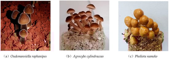
Figure 1.
Three different varieties of edible mushrooms: Oudemansiella raphanipes (OR), Agrocybe cylindraceas (AC) and Pholiota nameko (PN).
- (1)
- A novel edible mushroom synthetic cap occlusion image dataset generation method was proposed, which could automatically generate synthetic occlusion images and corresponding annotation in the realm of image processing. The method could also be applied to generate other amodal instance segmentation datasets and could effectively solve the problem in which the amodal ground truth cannot be obtained and greatly reduce the time for data collection and data annotation.
- (2)
- Based on the method of generating a synthetic image dataset, an Oudemansiella raphanipes, Agrocybe cylindraceas and Pholiota nameko amodal instance segmentation dataset was proposed to simulate a real-world dataset. It is the first synthetic edible mushroom image dataset for cap amodal instance segmentation.
- (3)
- An amodal mask-based method was proposed for calculating the width and length of caps. To the best of our knowledge, this is the first work that applies amodal instance segmentation to measure the width and length of caps based on synthetic training.
2. Materials and Methods
2.1. Raw Data Acquisition
The edible mushrooms used in this study were of three species: Agrocybe cylindraceas, Oudemansiella raphanipes and Pholiota nameko. Specifically, both the Agrocybe cylindraceas and Pholiota nameko were supplied by the Bioengineering and Technological Research Centre for Edible and Medicinal Fungi, Jiangxi Agricultural University. The Agrocybe cylindraceas contained 8 different varieties (JAUCC 0727, JAUCC 0532, JAUCC 2133, JAUCC 2135, JAUCC 1847, JAUCC 1920, JAUCC 1852, JAUCC 2110). The Oudemansiella raphanipes was cultivated in the edible mushroom factory in Zhangshu City, Jiangxi Province of China.
To accomplish our experiment, we chose a smart phone (Redmi K20 Pro, Xiaomi Technology Co., Ltd., Beijing, China) for data acquisition. For Agrocybe cylindraceass and Pholiota nameko, our workbench mainly consisted of a camera, a computer, and a light strip, as shown in Figure 2. Specifically, we fixed the view-point of the camera perpendicular to the mushroom bag and set a horizontal distance of 50 cm from the camera to the mushroom bag. For Oudemansiella raphanipe, we randomly shot from different perspectives and the distance was in the range from 10 to 30 cm. All RGB images were saved in JPEG format.
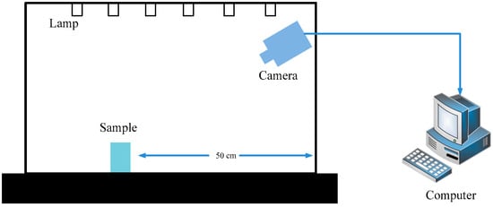
Figure 2.
The schematic of data acquisition workbench.
To validate whether the synthetic dataset can effectively be a substitute for a real cap occlusion dataset, we constructed two other subsets: one named subset A, which included 100 images with a fixed camera position and position of the mushroom bag and also included removal of the occluder cap to obtain the full shape of the occluded cap (ground truth). The other was named subset B, which was composed of images randomly selected from dataset A and contained a total of 300 occluded caps, annotated with occluded regions based on our experience.
2.2. Synthetic Image Generation and Annotation Method
The overview of the synthetic process is shown in Figure 3. First, to obtain the ground truth of the cap, we manually annotated cap images and saved the annotation information as a JSON file. Only the cap was needed in the subsequent step, so we intercepted the cap according to size of the cap. Furthermore, we generated the background image at a fixed size of 256 × 256, 512 × 512, 1024 × 1024 px, which ensured that the image covered the cap. All cap images were as a cap mask image pool (CMIP).
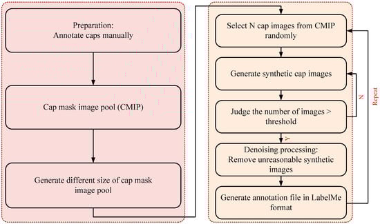
Figure 3.
Flowchart of the proposed synthetic cap occlusion image dataset method.
Then, we synthetized the high-throughput cap images. The detailed steps are as follows:
- (1)
- Select a cap mask image, , randomly as occluder and another . Images from CMIP were occluded.
- (2)
- As shown in Figure 4, calculate the position of the cap; we considered , , , , respectively, as the width and height of the bounding box of and . Furthermore, we set a movable area based on Equation (1) and generated a random point in the area of the circle with radius as the initial move position of the . The center of was mapped on according to the random point and then a mapped image was obtained.
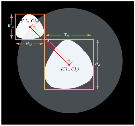 Figure 4. The schematic of cap position calculation.
 - (3)
- Occlusion processing. Based on step (2), iterate over the point of and ; we considered that if the point belongs both to and , then it is the occluded point, and then we removed it.
- (4)
- Denoising processing. As the synthetic image after step (3) sometimes has more than one region, we only maintained the largest region. Finally, combine the synthetic images and the Json file when annotated manually to generate a new Json file, which is suitable for LabelMe.
2.3. Amodal Instance Segmentation and Size Estimation
This study not only aims to rapidly generate synthetic cap occlusion images but also attempts de-occlusion for occluded mushrooms in situ. The flowchart of the de-occlusion process is shown in Figure 5. First, we used the synthetic image dataset to train and evaluate the amodal instance segmentation network. Then, we input an occluded cap binary image, which was cut into the same size as those of the training data. After feeding the pre-processed image into the trained model, a cap amodal mask was output. To restore the cropped mask coordinates, we created a new mask image, of which the size was the same as the input image, and calculated the cap mask image coordinates to visualize the predictions in RGB images. Furthermore, the coordinates were saved in the annotation file in the LabelMe format. Finally, the annotation file was visualized through the matlibplot library by converting the annotation file into the COCO format.
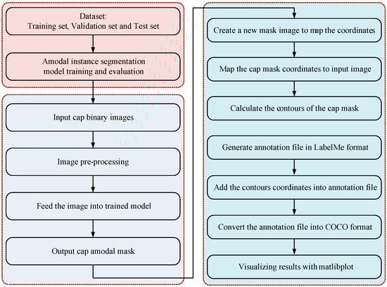
Figure 5.
Flowchart for acquiring the amodal segmentation mask and visualizing the RGB image.
2.3.1. Occlusion R-CNN
The Occlusion R-CNN (ORCNN) [15], which was extended from Mask R-CNN [16], added additional heads for the prediction of amodal masks (amodal mask head) and occlusion masks (occlusion mask head). It is a classic method for amodal instance segmentation, which aims to segment objects even if they are partially occluded or out of the image frame. The method consists of four main components, as shown in Figure 6: the backbone layers, the RPN module [17], the RoI module and the prediction branch. The backbone layers, composed of ResNet [18] and FPN [19] structures, are used to extract features from the input image and generate a coarse segmentation mask. The RPN networks typically consist of two branches: one for regressing bounding box offsets and the other for predicting target ness scores. These two branches share the convolutional feature extraction layer to generate candidate regions with different sizes at different scales and aspect ratios. According to the candidate regions generated by RPN, a RoI Pooling operation is performed on the feature map to map candidate regions of different sizes to a fixed-size feature map. This maintains the spatial information of the candidate regions [17]. The prediction branch includes four sub-branches: the classification branch, the bounding box regression branch, the visible mask branch and the amodal mask branch [15]. In our work, since our dataset is relatively homogeneous, we removed the first three branches and output only the amodal masks. The entire system was trained in an end-to-end manner using a combination of image-level classification loss and instance-level amodal segmentation loss. The model was trained on our synthetic cap occlusion image dataset to demonstrate the effectiveness of our synthetic image method.
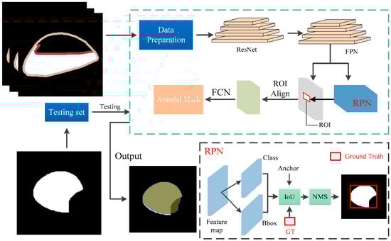
Figure 6.
Pipeline of deoccluded task. The part within the green dashed box represents the architecture of the ORCNN network. The output of ORCNN is the amodal mask of the occluded cap.
2.3.2. Size Estimation
Given an amodal mask of caps, the morphology phenotype parameters calculated by the bounding box would introduce systematic error, as shown in Figure 7a. We first used the principal component analysis (PCA) algorithm to acquire the main direction of the cap, as shown in Figure 7b. Then, we rotated the cap so that the main direction of the cap aligned with the image coordinate system, as shown in Figure 7c. Finally, we found that the length of the revised bounding box could be considered as the length of the cap, and the width could be acquired by calculating the valid pixel length of the cap center according to the width direction of the revised bounding box, shown approximatively in Figure 7d.
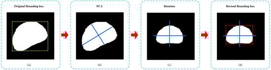
Figure 7.
The revising process of the bounding box of caps. (a) The original bounding box of amodal mask. (b) Computing the main direction using PCA algorithm. (c) Amodal mask after rotation with PCA. (d) The revised bounding box of rotated amodal mask.
2.4. Implementation Details
In our work, we utilized an Intel (R) Xeon (R) Silver 4214R @2.40 GHz CPU, 128 GB RAM, single-GPU computer (NVIDIA Quadro RTX 8000 with 48 GB memory). The software environment included python 3.7, a deep learning framework (Pytorch 1.4 [20]), CUDA 10.1, CUDNN 7.6.5, OpenCV 4 (ver. 4.7.0.72) and LabelMe 5.1 [21], which were installed in the Ubuntu 20.04 operation system. The model training and the synthetic image generation-related operation were accomplished on the same computer and environment.
2.5. Evaluation Metrics
To evaluate the performance of the edible mushroom instance segmentation model on the synthetic image dataset, average precision (AP) and recall (R) were applied in our work. Furthermore, AP is one of the most commonly used evaluation metrics in target detection, and it measures the performance by calculating the precision and recall at different confidence thresholds and then averaging the area under the precision–recall curve, while recall refers to the ability of the model to successfully find positive samples in the predicted results, which is usually applied in combination with AP.
To compute the value of AP and R, the Intersection over Union () was used in our work. Based on the overlapping area of the bounding box, the ranged from 0.5 to 0.95 with an interval of 0.05. Generally, AP50 and AP75 are the most common evaluation indicators when thresholds are 0.5 and 0.75, respectively. The definition of the bounding box’s and mask’s are depicted and the can be calculated by Equations (2) and (3).
To evaluate the performance of cap size estimation, the root mean square error () and the coefficient of determination () were introduced. The was computed by taking the square root of the mean of the squared differences between predicted values and manually labeled values. is a statistical measure that represents the proportion of the variance in the dependent variable that is predictable from the independent variables. The size estimation evaluation metrics were calculated by Equations (4) and (5), where represented the size of the sample, represented the manually labeled values, represented the predicted value and represented the average predicted value.
3. Results
3.1. Synthetic Cap Occlusion Image Dataset
We generated different scale sizes of the cap occlusion image dataset of 256 × 256, 512 × 512 and 1024 × 1024, respectively, and the cap was randomly covered with another cap, which indicated that the occlusion degree was randomly generated. Furthermore, we prepared a training dataset for each size per category of variety of synthetic occlusion image to fine-tune the amodal instance segmentation. The detail of the synthetic occlusion image dataset of caps is described in Table 1. Each training dataset was made up of 17,000 pairs of synthetic cap occlusion images and their corresponding masks, with 12,000 of those images used for training, 3000 for validation and 2000 for testing. The time consumption of image generation is shown in Table 1 for all the datasets of each image size of each category and some examples of the synthesized results are shown in Figure 8.

Table 1.
The detail of the occlusion image datasets for training, validation and testing generated by our synthetic image method.
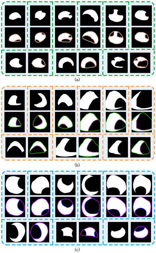
Figure 8.
Visualization results for synthetic cap occlusion images. (a) Agrocybe cylindraceas. (b) Oudemansiella raphanipes. (c) Pholiota nameko.
3.2. Amodal Instance Segmentation Results of Cap
The curves, including the training loss and validation loss curve of the model, of our synthetic cap occlusion image dataset, of 256 × 256 px, 512 × 512 px, 1024 × 1024 px, are shown in Figure 9, in which the backbone layer is ResNet50-FPN and ResNet101-FPN and for the pre-trained model is ImageNet weights. From Figure 9, we know that the model trained by each size of our synthetic dataset with ImageNet weights and the ResNet101-FPN backbone layer, including 4000 iterations, converges, and training and validation loss rapidly decrease between 0 and 1250 iterations and then become slower.
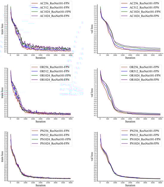
Figure 9.
The training process of with ResNet50 and ResNet101 with different sizes of images.
The model was evaluated using test datasets that included our synthetic occlusion image dataset with three different image sizes per category. Table 2 reports the quantified evaluation metrics of the model trained with ResNet101-FPN backbone and different image sizes (256 × 256, 512 × 512, 1024 × 1024 px) of our synthetic dataset, while Figure 9 illustrates examples of the amodal instance segmentation results for each category. From Table 2, we find that the AP@[0.5:0.95] of the model trained on Agrocybe cylindraceas (AC) and Oudemansiella raphanipes (OR) gradually decreases with the image size increases, but was still above 0.76. For Pholiota nameko (PN), the results of 256 × 256 px evaluated by the model trained on 512 × 512 and 1024 × 1024 px were only 0.51. Despite that, we applied the model trained with 256 × 256 px images per category to predict the test set and then visualized the results in RGB images, as shown in Figure 10.
Table 2.
The evaluated results of amodal instance segmentation using our synthetic dataset of different image sizes (256 × 256, 512 × 512, 1024 × 1024 px) with ImageNet weights and 4000 iterations.
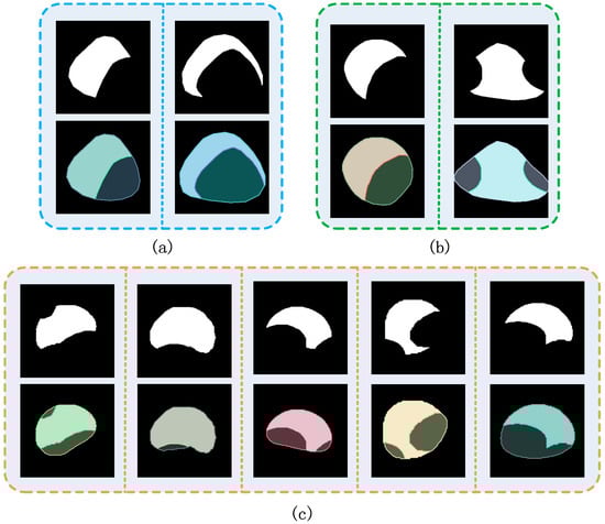
Figure 10.
Examples of amodal instance segmentation result. (a) Oudemansiella raphanipes. (b) Pholiota nameko. (c) Agrocybe cylindraceas.
Furthermore, the model was trained and evaluated on our synthetic image dataset with different backbone depths (ResNet50-FPN and ResNet101-FPN). Table 3 presents the quantified evaluation metrics of the model trained with the ResNet101-FPN and ResNet50-FPN backbone on our synthetic dataset with image sizes of 1024 × 1024 px. Some researchers have demonstrated that the ResNet101-FPN backbone can learn deeper features compared to the ResNet50-FPN backbone [16,18,22]. Generally, the deeper the layer is, the better the model is, but also the higher the number of parameters and cost. From Table 3, we found that both models where the backbone was ResNet50-FPN, as well as the model trained with the ResNet101-FPN backbone, worked well on our synthetic occlusion image dataset. We also found that regardless of if the backbone was ResNet50-FPN or ResNet101-FPN, each variety of AP@[0.5:0.95] decreased as the image size increased from 256 × 256 to 1024 × 1024 px. In addition, we applied the models to predict the test dataset and found that both output an excellent amodal mask. Additionally, some visualization results of amodal instance segmentation on RGB images are shown in Figure 11.
Table 3.
The evaluated results of amodal instance segmentation using our synthetic dataset of 1024 × 1024 px with ImageNet weights and 4000 iterations with different backbone layers.
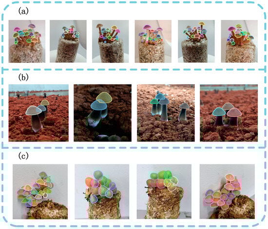
Figure 11.
Visualization results of amodal instance segmentation with RGB images. (a) Agrocybe cylindraceas. (b) Oudemansiella raphanipes. (c) Pholiota nameko.
3.3. Performance of the Models Trained on Different Datasets
To compare the performance of ORCNN on the synthetic dataset and the real dataset, we set up four subsets. The details of subset A and B were described in Section 2.1. Subset C included the training set and validation set, as shown in Table 1. Dataset D consisted of 300 images of occluded caps generated by our synthetic approach. Subset B, C and D were used to train and evaluate the amodal instance segmentation model, respectively, while dataset A was only used to evaluate the performance of the models. The results are shown in Table 4.
Table 4.
The evaluated results using dataset A, B, C and D.
From Table 4, we found that the average precision of the model trained on subset D was only 0.01 percentage points higher than that using subset B, both with the synthetic dataset and the manually labeled dataset. This demonstrates that our synthetic occlusion image dataset has the same performance as the manually labeled dataset on the ORCNN. Compared with the models trained on subset B, the model trained on dataset C had an AP of 0.97 percentage points, which was 0.18 percentage points higher than the former. This indicates that the addition of synthetic data increases the predictive ability of the model. In addition, we used the models trained on a small amount of data to predict the amodal masks of the occluded caps, as shown in Figure 12.
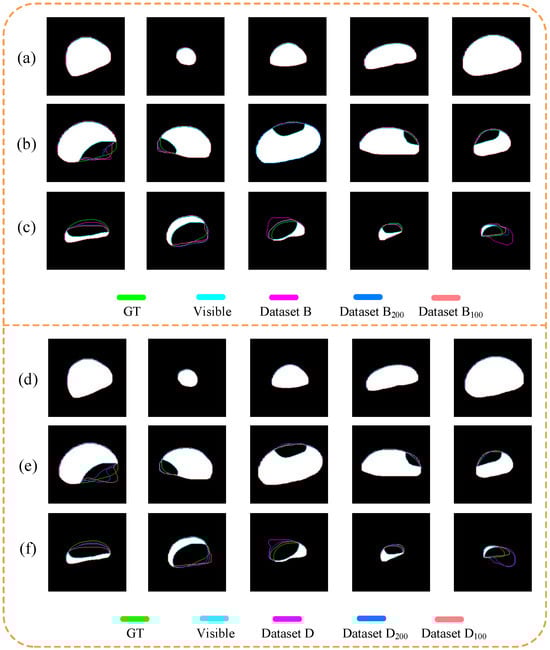
Figure 12.
Visualization results using datasets B (a–c) and D (d–f). (a,d) were non-occluded; (b,e) were slightly occluded; (c,f) were severely occluded.
3.4. Size Estimation of Caps
We selected different caps to generate occlusion images and then estimated the cap size based on the amodal masks, and the results of the cap length and width estimations are shown in Figure 13. The results indicate that the proposed method estimated that the width ( = 0.98) and length ( = 0.97) of the caps of AC had a fine linear relationship with the manually labeled data before PCA processing and had an = 0.96 and 0.99, respectively, after PCA processing. Moreover, the of the width and length of OR between the estimated measurement and manual measurement before PCA processing was 0.99 and 0.96, respectively, while after PCA processing, the was 0.99 and 0.96, respectively. In addition, the of the width and length of AC between the estimated measurement and manual measurement after PCA processing was 2.45 and 6.62, respectively, which decreased by 0.58 and 0.64 compared to the before PCA processing. The measurements based on our synthetic occlusion image dataset are almost the same as the manually labeled ones.
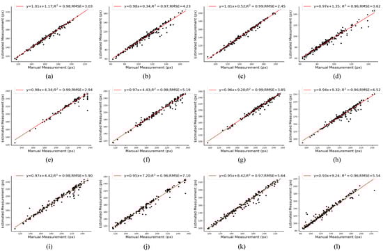
Figure 13.
Scatter plot and linear correlation of width and length between the manual measurement and estimated measurement. (a) The width of AC before PCA processing. (b) The length of AC before PCA processing. (c) The width of AC after PCA processing. (d) The length of AC after PCA processing. (e) The width of OR before PCA processing. (f) The length of OR before PCA processing. (g) The width of OR after PCA processing. (h) The width of OR after PCA processing. (i) The width of PN before PCA processing. (j) The length of PN before PCA processing. (k) The width of PN after PCA processing. (l) The length of PN after PCA processing.
4. Discussion
Regarding the edible mushroom occlusion cap image dataset generation task, the final dataset includes 12,000 images for training, 3000 images for validation and 2000 images for testing for each variety of Oudemansiella raphanipes, Agrocybe cylindraceas and Pholiota nameko. From Figure 8, we can find that the synthetic occlusion image dataset method can randomly generate occlusion cap images based on the non-occluded caps, which can simulate the visible region when the cap is occluded. The main reason for this is that we controlled the area for randomly generating the position of the upper cap and the center of the location of the upper cap was close to the edge of the occluded cap. However, there are also some cases that do not conform to the real occlusion. As shown in Figure 14a, no occlusion is generated. This is because the area of upper cap is bigger than the occluded cap and the placement of the upper cap generates randomly near to the center of occluded cap. Moreover, if two or more caps randomly generate occlusion to another cap, the situation in Figure 14b may occur. The reason for this is that the edge of the upper caps is adjacent to others, which results in a line in the middle of the occluded cap. Despite the fact that the synthetic occlusion image dataset method has the probability of generating the above implausible data, the majority of the data are still those of the actual occlusion situation. Furthermore, with enough normal data, these abnormal data have little effect on model training and evaluation.
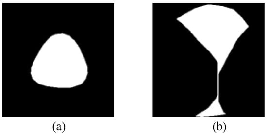
Figure 14.
Examples of an unreasonable synthetic occlusion image. (a) Synthetic image that without occlusion. (b) Synthetic image that the occlusion is unreasonable.
Furthermore, the amodal segmentation results showed an AP@[0.5:0.95] of 82%, 93% and 96% on the Oudemansiella raphanipes, Agrocybe cylindraceas and Pholiota nameko synthetic cap datasets, respectively, with a size of 1024 × 1024 px. Compared with [23], using the synthetic dataset results in a 17% improvement in amodal segmentation accuracy. Despite that, from Table 2, we learned that by using either the model trained with 512 × 512 or 1024 × 1024 px, the evaluation results of AP@[0.5:0.95] for 256 × 256 px are much lower for Agrocybe cylindraceas and Oudemansiella raphanipes. Meanwhile, the results of 512 × 512 and 1024 × 1024 px evaluated by the model trained with 256 × 256 px are also much lower than the results of 256 × 256 px. We hypothesize that the insufficient data of the original image used to generate the occluded image result in overfitting of the trained model. From Figure 10, it is obvious that the amodal instance segmentation model segments well on our cap synthetic occlusion image dataset. Despite the superior performance, there are some unsatisfactory results, as shown in Figure 15. The main reason is that the heavy occlusion results in a small visible region, which may output a myriad of cap fits. Unfortunately, heavy occlusion is common during the actual growth of edible mushrooms.
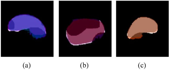
Figure 15.
Examples of amodal segmentation result where the mask is incomplete. (a–c) is three predicted amodal mask respectively that significantly different from the real shape.
From Figure 12, we can see that our size estimation method for cap length and width has a fine linear relationship with the manually labeled data. Despite that, there are still some estimated measurements that differ significantly from the manual measurements. The reasons are as follows: (1) Error introduced by manual measurement. We need to manually label a cap from the RGB image one by one and measure the cap length and width with the labeling results, which is prone to subjective errors. (2) Error introduced by the cap size estimation method. The cap length and width are measured by calculating the width of the bounding box, which is acquired by approximatively revising the bounding box, which can also introduce error. (3) Error introduced by amodal segmentation. The cap length and width size estimation rely on the results of the amodal segmentation, while the results of the PCA algorithm will vary slightly with the amodal segmentation results. Unfortunately, if the cap is heavily occluded, the only non-occluded region can fit countless caps, which can differ largely from the labeled cap and introduce error. Additionally, our edible mushroom size estimation method is pixel-based, which lacks the depth distance to transform from image to world coordinates.
5. Conclusions
The proposed method can be used in automatic high-throughput edible mushroom cap phenotype research, which solves the difficulty of not being able to obtain the complete shape of occluded caps from one image view-point and provides a quicker and more precise annotation method for experts to reduce time costs. For growers and breeders, our method provides rapid access to cap phenotypic parameters, providing a rich reference of data for growth monitoring and breeding designs. Additionally, farmers can apply it to quickly estimate mushroom yields.
However, our methods have a few limitations. Firstly, we always try to measure the caps quickly and with high precision, and therefore we only use the RGB images for study, ignoring the effect of the depth information on the accuracy. Secondly, our synthetic image approach is limited to the object, of which the shape is simple; thus, our methods still need to be improved for complex shaped targets. In our future research, constructing datasets that contain depth information is a priority. Additionally, other research on methods for analyzing the phenotypic parameters of edible mushrooms in complex environments is necessary.
Author Contributions
Q.W.: Data curation, Methodology, Formal analysis, Writing—original draft; Y.W.: Supervision, Writing—review and editing; S.Y.: Data curation, Methodology; C.G.: Data curation, Methodology; L.W.: Data curation, Methodology; H.Y.: Writing—review and editing, Project administration, Supervision. All authors have read and agreed to the published version of the manuscript.
Funding
This study was supported by the National Natural Science Foundation of China (62362039), Graduate Student Innovation Fund project (YC2023-S366), Innovation and Entrepreneurship Training Program for College Students project (202410410016X).
Data Availability Statement
Given that the data used in this study were self-collected, the dataset is being further improved. Thus, the dataset is unavailable at present.
Acknowledgments
Special thanks to the reviewers for their valuable comments.
Conflicts of Interest
The authors declare no conflicts of interest.
References
- Wang, Y.X.; Zhang, T.; Huang, X.J.; Yin, J.Y.; Nie, S.P. Heteroglycans from the Fruiting Bodies of Agrocybe Cylindracea: Fractionation, Physicochemical Properties and Structural Characterization. Food Hydrocoll. 2021, 114, 106568. [Google Scholar] [CrossRef]
- Zhang, J.; Chen, X.; Mu, X.; Hu, M.; Wang, J.; Huang, X.; Nie, S. Protective Effects of Flavonoids Isolated from Agrocybe Aegirita on Dextran Sodium Sulfate-Induced Colitis. eFood 2021, 2, 288–295. [Google Scholar] [CrossRef]
- Li, S.; Yan, Z.; Guo, Y.; Su, X.; Cao, Y.; Jiang, B.; Yang, F.; Zhang, Z.; Xin, D.; Chen, Q.; et al. SPM-IS: An Auto-Algorithm to Acquire a Mature Soybean Phenotype Based on Instance Segmentation. Crop J. 2022, 10, 1412–1423. [Google Scholar] [CrossRef]
- Van De Vooren, J.G.; Polder, G.; Van Der Heijden, G.W.A.M. Application of Image Analysis for Variety Testing of Mushroom. Euphytica 1991, 57, 245–250. [Google Scholar] [CrossRef]
- Van De Vooren, J.G.; Polder, G.; Van Der Heijden, G.W.A.M. Identification of Mushroom Cultivars Using Image Analysis. Trans. ASAE 1992, 35, 347–350. [Google Scholar] [CrossRef]
- Tanabata, T.; Shibaya, T.; Hori, K.; Ebana, K.; Yano, M. American Society of Plant Biologists (ASPB) Smart-Grain: High-Throughput Phenotyping Software for Measuring Seed Shape through Image Analysis. Physiology 2012, 160, 1871–1880. [Google Scholar] [CrossRef]
- Zhao, M.; Wu, S.; Li, Y. Improved YOLOv5s-Based Detection Method for Termitomyces Albuminosus. Trans. Chin. Soc. Agric. Eng. 2023, 39, 267–276. [Google Scholar] [CrossRef]
- Yin, H.; Xu, J.; Wang, Y.; Hu, D.; Yi, W. A Novel Method of Situ Measurement Algorithm for Oudemansiella Raphanipies Caps Based on YOLO v4 and Distance Filtering. Agronomy 2023, 13, 134. [Google Scholar] [CrossRef]
- Yang, S.; Zheng, L.; Yang, H.; Zhang, M.; Wu, T.; Sun, S.; Tomasetto, F.; Wang, M. A Synthetic Datasets Based Instance Segmentation Network for High-Throughput Soybean Pods Phenotype Investigation. Expert Syst. Appl. 2022, 192, 116403. [Google Scholar] [CrossRef]
- Lin, T.-Y.; Maire, M.; Belongie, S.; Hays, J.; Perona, P.; Ramanan, D.; Dollár, P.; Lawrence Zitnick, C.; Irvine, U. Microsoft COCO: Common Objects in Context. In Proceedings of the Computer Vision—ECCV 2014: 13th European Conference, Zurich, Switzerland, 6–12 September 2014; Proceedings, Part IV. Springer: Cham, Switzerland, 2014. [Google Scholar]
- Xu, P.; Fang, N.; Liu, N.; Lin, F.; Yang, S.; Ning, J. Visual Recognition of Cherry Tomatoes in Plant Factory Based on Improved Deep Instance Segmentation. Comput. Electron. Agric 2022, 197, 106991. [Google Scholar] [CrossRef]
- Zhou, W.; Chen, Y.; Li, W.; Zhang, C.; Xiong, Y.; Zhan, W.; Huang, L.; Wang, J.; Qiu, L. SPP-Extractor: Automatic Phenotype Extraction for Densely Grown Soybean Plants. Crop J. 2023, 11, 1569–1578. [Google Scholar] [CrossRef]
- Kuznichov, D.; Zvirin, A.; Honen, Y.; Kimmel, R. Data Augmentation for Leaf Segmentation and Counting Tasks in Rosette Plants. In Proceedings of the IEEE Computer Society Conference on Computer Vision and Pattern Recognition Workshops, Long Beach, CA, USA, 16–17 June 2019; IEEE Computer Society: Washington, DC, USA, 2019; pp. 2580–2589. [Google Scholar]
- Toda, Y.; Okura, F.; Ito, J.; Okada, S.; Kinoshita, T.; Tsuji, H.; Saisho, D. Training Instance Segmentation Neural Network with Synthetic Datasets for Crop Seed Phenotyping. Commun. Biol. 2020, 3, 173. [Google Scholar] [CrossRef] [PubMed]
- Follmann, P.; König, R.; Härtinger, P.; Klostermann, M. Learning to See the Invisible: End-to-End Trainable Amodal Instance Segmentation. In Proceedings of the IEEE Winter Conference on Applications of Computer Vision 2019, Waikoloa, HI, USA, 7–11 January 2019; pp. 1328–1336. [Google Scholar] [CrossRef]
- He, K.; Gkioxari, G.; Dollar, P.; Girshick, R. Mask R-CNN. In Proceedings of the IEEE International Conference on Computer Vision 2017, Venice, Italy, 22–29 October 2017; pp. 2961–2969. [Google Scholar] [CrossRef]
- Ren, S.; He, K.; Girshick, R.; Sun, J. Faster R-CNN: Towards Real-Time Object Detection with Region Proposal Networks. IEEE Trans. Pattern Anal. Mach. Intell. 2017, 39, 1137–1149. [Google Scholar] [CrossRef] [PubMed]
- He, K.; Zhang, X.; Ren, S.; Sun, J. Deep Residual Learning for Image Recognition. In Proceedings of the 2016 IEEE Conference on Computer Vision and Pattern Recognition (CVPR), Las Vegas, NV, USA, 27–30 June 2016. [Google Scholar]
- Long, J.; Shelhamer, E.; Darrell, T. Fully Convolutional Networks for Semantic Segmentation. IEEE Trans. Pattern Anal. Mach. Intell. 2017, 39, 640–651. [Google Scholar] [CrossRef] [PubMed]
- Paszke, A.; Gross, S.; Massa, F.; Lerer, A.; Bradbury Google, J.; Chanan, G.; Killeen, T.; Lin, Z.; Gimelshein, N.; Antiga, L.; et al. PyTorch: An Imperative Style, High-Performance Deep Learning Library. Adv. Neural Inf. Process. Syst. 2019, 32, 8026–8037. [Google Scholar] [CrossRef]
- Russell, B.C.; Torralba, A.; Murphy, K.P.; Freeman, W.T. LabelMe: A Database and Web-Based Tool for Image Annotation. Int. J. Comput. Vis. 2008, 77, 157–173. [Google Scholar] [CrossRef]
- Igathinathane, C.; Pordesimo, L.O.; Columbus, E.P.; Batchelor, W.D.; Methuku, S.R. Shape Identification and Particles Size Distribution from Basic Shape Parameters Using ImageJ. Comput. Electron. Agric. 2008, 63, 168–182. [Google Scholar] [CrossRef]
- Yin, H.; Wei, Q.; Gao, Y.; Hu, H.; Wang, Y. Moving toward Smart Breeding: A Robust Amodal Segmentation Method for Occluded Oudemansiella Raphanipes Cap Size Estimation. Comput. Electron. Agric. 2024, 220, 108895. [Google Scholar] [CrossRef]
Disclaimer/Publisher’s Note: The statements, opinions and data contained in all publications are solely those of the individual author(s) and contributor(s) and not of MDPI and/or the editor(s). MDPI and/or the editor(s) disclaim responsibility for any injury to people or property resulting from any ideas, methods, instructions or products referred to in the content. |
© 2024 by the authors. Licensee MDPI, Basel, Switzerland. This article is an open access article distributed under the terms and conditions of the Creative Commons Attribution (CC BY) license (https://creativecommons.org/licenses/by/4.0/).