Article

Geographical Environment and Plant Functional Group Shape the Spatial Variation Pattern of Plant Carbon Density in Subalpine-Alpine Grasslands of the Eastern Loess Plateau, China

by
Manhou Xu
1,2,3,*,
Jiaying Wang
1,
Kunkun Wei
1,
Jie Li
1 and
Xiuli Yu
1,2,3
1
School of Geographic Sciences, Taiyuan Normal University, Jinzhong 030619, China
2
Institute of Carbon Neutrality, Taiyuan Normal University, Jinzhong 030619, China
3
Shanxi Key Laboratory of Earth Surface Processes and Resource Ecology Security in Fenhe River Basin, Taiyuan Normal University, Jinzhong 030619, China
*
Author to whom correspondence should be addressed.
Agronomy 2024, 14(7), 1420; https://doi.org/10.3390/agronomy14071420
Submission received: 30 May 2024 / Revised: 22 June 2024 / Accepted: 28 June 2024 / Published: 29 June 2024
(This article belongs to the Special Issue Advances in Grassland Productivity and Sustainability — 2nd Edition)

Abstract

:
The carbon density of subalpine-alpine grasslands (SGs) is significantly vital to sustaining the carbon cycle in global terrestrial ecosystems. However, on the Loess Plateau of China, it remains unclear how the geographical environment and plant functional groups affect the spatial variation pattern of plant carbon density in these grasslands. Here, nine typical SGs distributed in the eastern Loess Plateau with elevations ranging from 1720 to 3045 m were investigated. The biomass indices from grassland plants of different functional groups were investigated using plot surveys. The Kriging interpolation method was used to explore the spatial variation pattern of plant carbon density along geographical gradients. We found that (1) the total plant carbon density of SGs was 2676.825 g C/m2 on the eastern plateau, with 37.07%, 37.50%, and 25.43% contributed by the northern, central, and southern areas, respectively. Above- (666.338 g C/m2) and belowground (2010.488 g C/m2) carbon density accounted for 24.9% and 75.11% of the total, respectively. (2) At the horizontal scale, the plant carbon density in the northern SGs was high in the northwest and low in the southeast; in the central SGs, it was low in the northwest and high in the southeast; and in the southern SGs, it was high in the southwest and low in the northeast. At the vertical scale, plant carbon density in all SGs decreased with increasing altitude. (3) The carbon density of grasses, forbs, and sedges was 247.419 g C/m2, 26.073 g C/m2, and 23.471 g C/m2, respectively. With increased latitude, the carbon density of all functional groups (grasses, forbs, and sedges) decreased; the carbon density of forbs and grasses increased with increased longitude, while that of sedges decreased; and with increased altitude, the carbon density of all functional groups increased. In conclusion, the spatial variation pattern of plant carbon density in the SGs was not only influenced by the geographical environment but also by the plant functional groups at the horizontal and vertical scales on the eastern Loess Plateau of China.

1. Introduction

Natural ecosystems store large amounts of carbon globally, as organisms absorb carbon from the atmosphere to build large, long-lasting, or slow-decaying structures such as tree bark or root systems [1,2]. An ecosystem’s carbon sequestration potential is tightly linked to its biological diversity. Yet when considering future projections, many carbon sequestration models fail to account for the role biodiversity plays in carbon storage [1]. Hundreds of experimental studies have consistently found that within a place, more diverse assemblages, and in particular more diverse plant assemblages, have higher standing biomass production and carbon sequestration [1].
Grasslands, as an important component of the global terrestrial ecosystem, have a wide distribution area and are the main source of organic carbon input in the terrestrial ecosystem [2]. They therefore play an important role in the carbon cycle. According to statistics, the carbon storage of global grassland ecosystems is second only to that of forests, with a total amount of 761 Gt, and accounts for 34% of the global carbon storage [3]. In China, the area of grassland is about 400 million hm2, comprising 40% of the total land area; it has a carbon storage of 44.09 Gt, accounting for about 8% of the world’s grassland ecosystem carbon storage [4]. This demonstrates that grasslands have a strong capacity for carbon sequestration. Therefore, they play a pivotal role in the national “two carbon” goals (peak carbon and carbon neutrality) in China.
Carbon density is an important index for measuring the carbon storage in a certain area, and the vegetation biomass of grasslands could be used to estimate their plant carbon density [5]. Many scholars have conducted studies on the estimation of grassland carbon density from plant and soil aspects [6,7,8]. They found that compared with grasslands, the total forest carbon sink was the largest among terrestrial ecosystems [9], and the global soil organic carbon pool was about 1359 × 1015 g [10]. However, plant management measures for grasslands could alleviate the decline in soil carbon sequestration caused by plant degradation [8]. Among these studies, grassland carbon density was mainly estimated by establishing a net primary productivity (NPP) model or using remote sensing technology [11]. Therefore, it is of great practical significance to estimate grassland carbon density and explore its distribution with spatial analyses.
In China, previous studies on the plant carbon pools of grassland ecosystems were mainly concentrated in Inner Mongolia [12,13] and the Qinghai-Tibet Plateau [3,14]. A small number of studies have been conducted in other regions, such as Xinjiang [15] and the Loess Plateau [16]. Studies on carbon density in the Loess Plateau mainly focused on lowland grasslands [17] and forest ecosystems [18] in low-altitude regions and rarely focused on subalpine-alpine grasslands (SGs) in high-altitude mountains. Chen [17] sampled 70 grassland plots in Shanxi Province and measured above- and belowground biomass. It was found that the total carbon density of the grassland ecosystem in Shanxi Province was 2718.53–13,260.6 g C/m2. A study by Qiao [19] showed that the carbon density of soil, roots, ground living, and litter in Shanxi grasslands accounted for 78.67%, 19.76%, 1.25%, and 0.32% of the total, respectively. Zhang et al. [20] also estimated the total carbon storage of typical grasslands in Shanxi Province at 364.40 Tg, in which the average carbon density was 1759.07 g C/m2 for vegetation and 6307.22 g C/m2 for soil. These studies found that the proportion of soil carbon density in grassland ecosystems was much higher than that of plant carbon density. However, there were some differences in the estimation of grassland carbon density, which might have been caused by different calculation methods, experimental plots, and plant functional groups [21,22]. For example, a study on the spatial variation in plant functional groups and biodiversity in various functional zones showed that the biomass of perennial grasses and forbs of the plant community in the three zones declined in the order of core zone > buffer zone > experimental zone, while that of shrubs and annual grasses increased in reverse order [2]. Another study on the effects of soil physical and chemical properties on the aboveground biomass of functional groups at different degradation successional stages of alpine meadows also illustrated significantly low and high aboveground biomass for sedges and forbs, respectively; however, there was no significant difference in the aboveground biomass of grasses [23]. These findings indicated that various plant functional groups also had effects on the carbon density of grassland ecosystems.
As mentioned above, few studies on grassland carbon density in the Loess Plateau of China have focused on SGs in high-altitude mountains. SGs are one type of terrestrial grassland that are mainly distributed in high-altitude mountains, where species diversity and biomass are affected by the mountainous terrain [24]. Latitude, longitude, and altitude are the dominant terrain indicators of SGs; these indicators directly affect the spatial distribution of solar radiation and rainfall and thus result in an uneven distribution of soil moisture and temperature [25,26]. Shanxi Province, located in the east of the Loess Plateau, is an important province in central China that plays a vital role in the ecological conservation strategy and high-quality development of the Yellow River Basin. Owing to its geographical location on the Loess Plateau, Shanxi Province has become a region with serious soil erosion and a fragile environment, and its vegetation has typical geographical gradient distribution characteristics [24]. SGs are distributed over a large area in Shanxi Province. These grasslands not only provide excellent natural pastures but also serve as famous eco-attractions. For example, Heyeping has been honored as the “jade plateau”, Shunwangping as the “Jiuzhaigou of north China”, and the Wutai Mountain as “the roof of north China” [24]. However, with global warming and the development of human activities (e.g., cattle grazing), SGs in the eastern part of the Loess Plateau are undergoing an accelerated degradation of productivity [24,26]. Therefore, it is necessary to explore the plant carbon density of SGs together with its spatial variation pattern along geographical gradients.
We conducted field surveys on these SGs in the plant growing season, and the plant biomass of SGs with different functional groups was investigated in the mountain systems of Liuleng, Wutai, Lvliang, and Zhongtiao in the east of the Loess Plateau. The aims of this research were (1) to estimate the plant carbon density of SGs with different functional groups and (2) to probe the spatial variation pattern of plant carbon density along different geographical gradients. It was hypothesized that the spatial variation pattern of plant carbon density in SGs is shaped collectively by the geographical environment and plant functional groups.

2. Materials and Methods
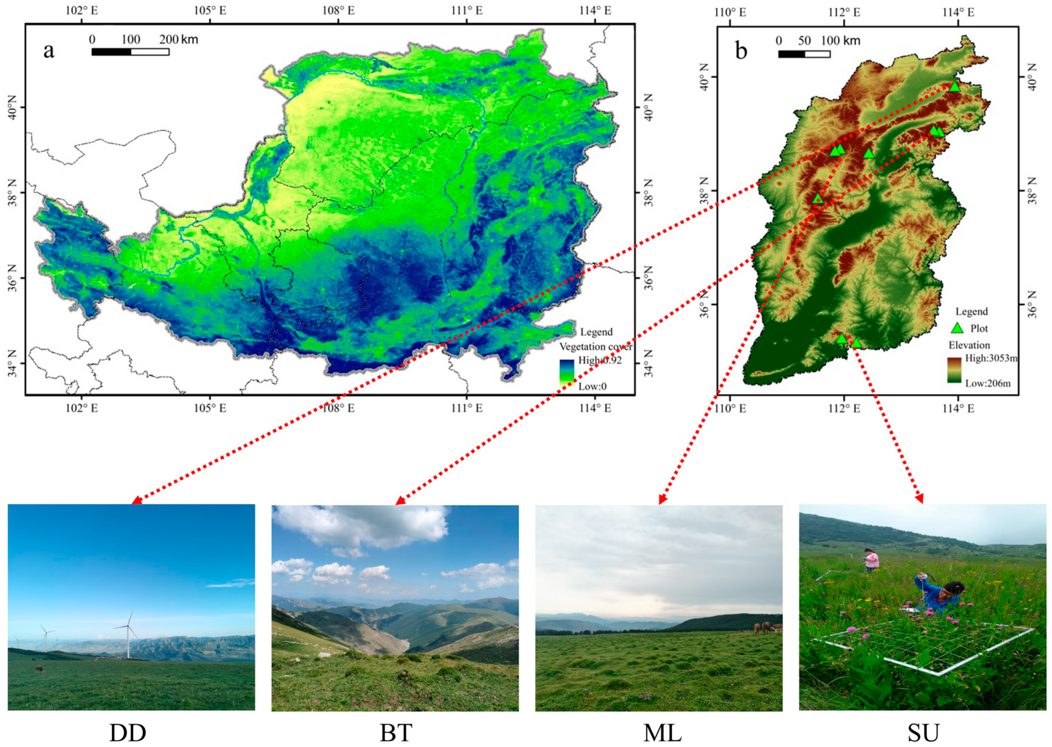
2.1. Study Area

The Loess Plateau (Figure 1a) of China contains the largest area of loess in the world and is characterized by scarce precipitation, intense evaporation, severe soil erosion, and a low ability to resist natural hazards. The environmental conditions are therefore harsh, and it is extremely difficult to restore degraded areas. The east of the plateau (34°34′–40°43′ N, 110°14′–114°33′ E) lies in Shanxi Province (Figure 1b) and serves as a dividing line between the second and third steps of topography in China. This location also contains the greatest concentration of SGs in the entire plateau. Owing to the complex and changeable topography, the Taihang and Lvliang mountains and a series of basins between them are found in this area. From north to south, these basins are successively named the Datong, Xinding, Taiyuan, Changzhi, Linfen, and Yuncheng basins [26]. The temperate continental monsoon climate features annual, summer, and winter mean temperatures of 4–14 °C, 22–27 °C, and −12 to −2 °C, respectively; an annual precipitation of 400–600 mm; and a frost-free season of 4–7 months [24]. The dominant vegetation in this region is typical of temperate regions with complicated geomorphic features and combinations of water and heat. Mountainous areas occupy more than 80% of this region, and SGs cover around 353,000 hm2 of the larger mountain systems; these are mainly distributed in high-altitude belts above the timberline in the Liuleng, Lvliang, Wutai, and Zhongtiao systems [24]. The plants in SGs principally include perennial herbs that are suitable for low temperatures and moderate moisture, including the Carex and Kobresia genera.

2.2. Experimental Design

Comparing with a vegetation-type map of the Loess Plateau (Figure 1a) and a topographic map of Shanxi Province in China (Figure 1b), SGs on nine mountains were investigated from July to August in the summer of 2023, namely, Dianding (DD) in the Liuleng mountain system; Beitai (BT) and Dongtai (DT) in the Wutai mountain system; Malun (ML), Heyeping (HY), Yunzhong (YZ), and Yunding (YD) in the Lvliang mountain system; and Shunwangping (SU) and Shengwangping (SE) in the Zhongtiao mountain system (Table 1). These mountains have typical SGs with a large area and facilitate relatively easy plant sampling. Among these mountains, DD, BT, and DT were geographically classified as northern; ML, HY, YZ, and YD as central; and SU and SE as southern mountains in Shanxi Province [24].
Additionally, prior to conducting this experiment, permission was obtained in a 2016 field survey from the Luyashan National Nature Reserve (Xinzhou City) for DD, BT, and DT; the Pangquangou National Nature Reserve (Lvliang City) for ML, HY, YZ, and YD; and the Wulushan National Nature Reserve (Linfen City) for SU and SE. These cities are all in Shanxi Province of China. This permission was obtained successfully, as the field studies did not involve endangered or protected plant species.

2.3. Measurement of Plant Biomass

Five plots were set up randomly at each of the nine mountain sites to measure plant diversity and biomass, with forty-five plots in total. Each plot had a size of 1 m2 due to the sampling on herbaceous communities, and 5 m2 in total was for each mountain site. The herbaceous species in the study site were categorized into three major plant functional groups: sedges, grasses, and forbs [21,22]. The life forms of various species were confirmed with reference to the Flora of China (http://www.iplant.cn/ (accessed on 23 September 2013)).
After investigating plant species diversity, the live plant biomass was surveyed at the individual scale in the growing season. Plant litters were not sampled for biomass, as they were difficult to be separated from different functional groups. A patch containing the whole or overwhelming majority of the root system was excavated with a spade. Patch size and shape were determined by the root morphology of each species. Usually, a 10–20 cm diameter patch of grass was excavated to a depth of 20–30 cm [27,28]. After that, the whole individual of each plant species was separated from soil, and the soil was filled back into those holes excavated by the spade. The filled holes were packed tightly again. The aim of this operation was to avoid the degradation of SGs due to anthropogenic actions.
The roots of each sample were carefully separated from the soil and other belowground material. Live roots were distinguished from dead roots by their colors, consistency, and the presence or absence of attached fine roots [27]. Then, live roots and shoots were separated and placed into separate paper envelopes. Afterward, the live roots were washed free of soil under running water (<5 °C) before all plant samples were oven-dried at 80 °C to a constant mass in the laboratory; next, plant above- and belowground biomass of each species was recorded using an electronic balance with an accuracy of 0.001 g. Finally, individual surveys of plant above- and belowground biomass were averaged for each species for each plot. Therefore, aboveground biomass, belowground biomass, and total biomass were calculated for sedges, grasses, and forbs, respectively.

2.4. Data Analysis

2.4.1. Estimation of Plant Carbon Density

The sum of the measured aboveground and belowground biomass was taken as the total. Using the above- and belowground and total biomass of vegetation, the carbon density of the plants in the SGs was estimated for each of the mountains. The estimation of plant carbon density is usually converted to carbon content in terms of the proportion of carbon in vegetative organic matter [29]. However, the conversion rate varies for different vegetation types (such as trees, shrubs, vine plants, and herbaceous plants), and it is very limited for obtaining the conversion rate of these types of vegetation. Here, we referred to the results for carbon content of herbaceous plants in the book Methods Manual for Measuring Terrestrial Carbon by Winlock International in 2005 [30]. This study adopted the conversion rate of 0.45 in the book for herbaceous plants, which was commonly used in international studies to convert biomass indices with the form of carbon (g C/m2). The sum of the above- and belowground carbon density was taken as the total carbon density in the region. The converted equation is shown below.
C = C A G + C B G
C A G = A G B × 0.45
C B G = B G B × 0.45
where C represents the plant total carbon density, g C/m2; CAG and CBG represent the plant above- and belowground carbon density, g C/m2; and AGB and BGB represent the plant above- and belowground biomass, g/m2, respectively.

2.4.2. Spatial Interpolation of Plant Carbon Density

The Kriging method is the most commonly used method for spatial interpolation in geostatistical analyses [25]. Based on the coefficient of variation, this method can achieve linear unbiased optimal estimation of a variable’s position in a certain region. After all data predictions are completed, the interpolation results can be cross-verified based on the original data points [31]. Therefore, the Kriging method is more suitable for the spatial interpolation of plant carbon density and has higher accuracy than other methods [32,33].
The statistical analysis module in ArcGIS 10.8 (ESRI Inc., Redlands, CA, USA) was used to perform the Kriging interpolation of the plant carbon density of SGs with different functional groups (namely the sedges, grasses, and forbs), to predict the plant carbon density of unknown SGs, and then to draw spatial distribution maps with different functional groups. Before interpolation, a histogram was first used to check whether the normal distribution was suitable. Second, a QQ chart was used to verify whether the data were consistent with a straight line. Third, the Tyson polygon was used to check whether there were abnormal values that should be eliminated. Fourth, a trend analysis was used to determine whether the plant carbon storage data exhibited a “U” shape.
When interpolation was conducted, in the step of geostatistical method selection, the ordinary Kriging and prediction map were selected. Then, a spherical model was chosen as the variation function model with no anisotropy. The nugget, partial sill, and major range were obtained for the variation function by adjusting the number of lags and lag size. In the final step of cross validation, the average error and root mean square error of each model were compared to make them close to 0 and 1, respectively, and then, the optimal model was selected to complete the spatial interpolation of the plant carbon density of SGs.

3. Results

3.1. Estimation of Plant Carbon Density of SGs

The plant carbon density of SGs was mainly distributed in the Taihang and Lvliang mountains, with relatively little in the middle six basins (Figure 2a). The above- and belowground and total carbon density values of the SGs were 666.338 g C/m2, 2010.488 g C/m2, and 2676.825 g C/m2, respectively (Table 2).
The above- and belowground carbon density fluctuated in the range of 24.683–155.228 g C/m2 and 116.123–354.533 g C/m2, respectively, and the total ranged from 164.205 to 460.395 g C/m2 (Table 2).
The aboveground carbon density showed an increasing trend from DD to SE, among which HY, SU, and SE showed large values of 105.863 g C/m2, 131.918 g C/m2, and 155.228 g C/m2, respectively, and the minimum value was found in the central YD (24.683 g C/m2) (Table 2). The aboveground carbon density in the southern mountains (287.145 g C/m2) was significantly higher than that in the northern (151.673 g C/m2) and central (227.520 g C/m2) mountains (Figure 2a).
The belowground carbon density showed a decreasing trend, with large values in DD (248.558 g C/m2), BT (405.630 g C/m2), and HY (354.533 g C/m2) in the central mountains and SE (206.438 g C/m2) in the southern mountains (Table 2). The belowground carbon density values in the northern and central mountains were 447.075 g C/m2 and 383.04 g C/m2, respectively, which were significantly higher than those in the southern mountains (Figure 2a).
There was no obvious change trend in the total carbon density. The largest values were found in BT and HY at 444.128 g C/m2 and 354.533 g C/m2, respectively, while the smaller values were found in YZ (180.653 g C/m2) and YD (164.205 g C/m2) (Table 2). The total carbon density in the southern mountains (680.603 g C/m2) was significantly lower than that in the northern (992.205 g C/m2) and central (1004.018 g C/m2) mountains (Figure 2a).
In general, from north to south, the aboveground carbon density showed an increasing trend, while the belowground and total carbon density showed a decreasing trend (Figure 2a).

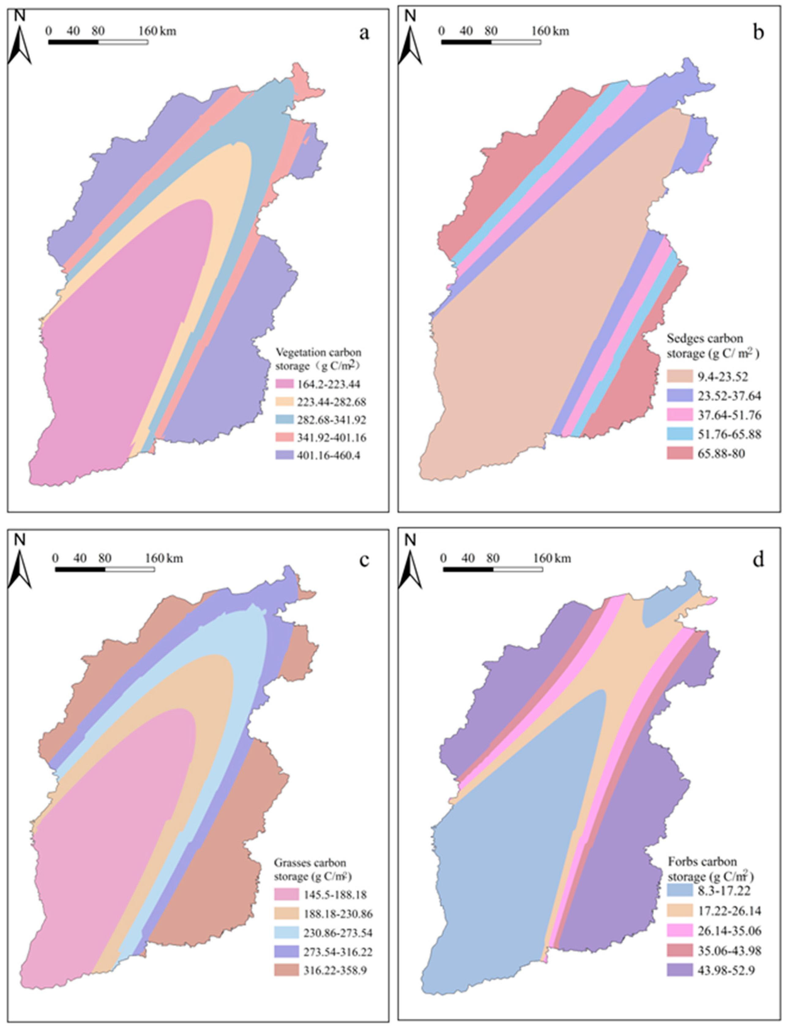
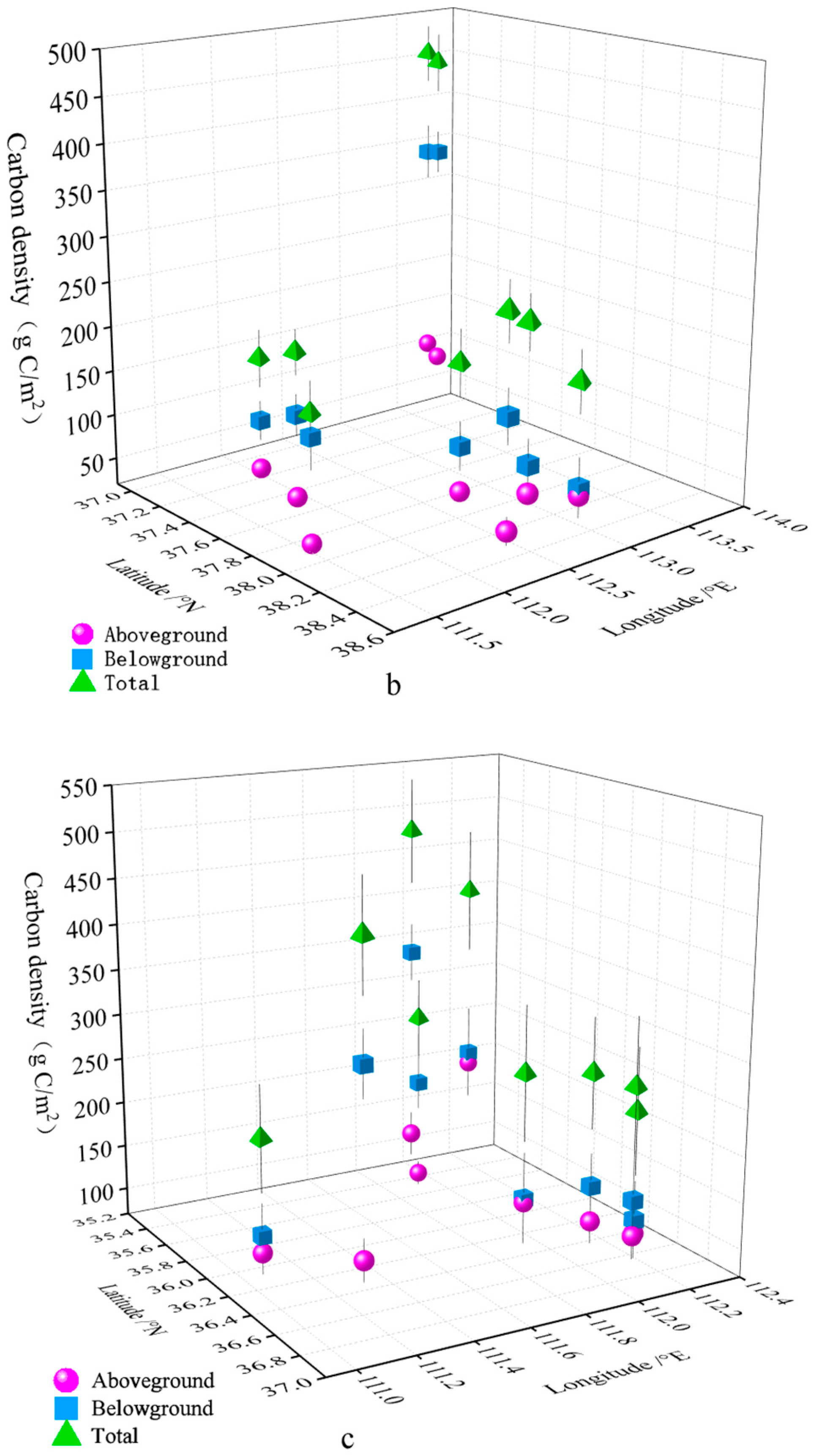
3.2. Spatial Distribution Characteristics of Plant Carbon Density in SGs

In the horizontal direction, the plant carbon density of the northern, central, and southern SGs increased from southeast to northwest, northwest to southeast, and northeast to southwest, respectively. In other words, the plant carbon density of the northern SGs was high in the northwest and low in the southeast, that of the central SGs was high in the southeast and low in the northwest, and that of the southern SGs was high in the southwest and low in the northeast (Figure 3).
In the northern mountains, the plant aboveground carbon density decreased, the plant belowground carbon density increased, and the plant total carbon storage increased with the increase in latitude. With the increase in longitude, the plant above- and belowground and total carbon density showed a decreasing trend (Figure 3a).
In the central mountains, the plant aboveground carbon density increased with the increase in latitude, while the plant belowground and total carbon density both decreased. With the increase in longitude, the plant above- and belowground and total carbon density showed an increasing trend (Figure 3b).
In the southern mountains, the plant above- and belowground and total carbon density decreased with the increase in latitude. With the increase in longitude, the plant aboveground carbon density showed an increasing trend, while the plant belowground and total carbon density showed a decreasing trend (Figure 3c).
In the vertical direction, the plant total carbon density in the northern (Figure 4a), central (Figure 4b), and southern (Figure 4c) mountains decreased with the increase in altitude (p > 0.05). In the northern and southern mountains, the plant aboveground, belowground, and total carbon density decreased with the increase in altitude (p > 0.05). With the increase in elevation, the plant aboveground carbon density showed an increasing trend, while the plant belowground and total carbon density showed a decreasing trend (p > 0.05) (Figure 4).

3.3. Spatial Variations in Plant Carbon Density with Different Functional Groups in SGs

On the whole, the plant aboveground, belowground, and total carbon density of grasses were significantly higher than those of forbs and sedges. For forbs, the aboveground carbon density ranged from 1.407 to 16.920 g C/m2; the belowground carbon density ranged from 4.863 to 46.647 g C/m2; and the total carbon density ranged from 8.292 to 52.945 g C/m2 (Table 3). For sedges, the maximum plant aboveground, belowground, and total carbon density were 16.303 g C/m2, 54.598 g C/m2, and 70.901 g C/m2, respectively (Table 3). For grasses, the minimum values of plant aboveground, belowground, and total carbon density were 21.869 g C/m2, 100.678 g C/m2, and 145.486 g C/m2, respectively (Table 3). The aboveground carbon density data for forbs and sedges were aggregated with the belowground carbon density data, whereas the aboveground, belowground, and total carbon density data for grasses were discrete. This variation in the data for plant carbon density with different functional groups illustrated that different individuals of forbs, sedges, and grasses had greater differences in responses to the geographical environment due to their diverse biological characteristics.
The carbon density of grasses was the highest in DD (129.925 g C/m2), significantly higher than that in YZ and YD, and the lowest in YZ (21. 869 g C/m2) (Figure 5a). The DD carbon density (16.92 g C/m2) in the aboveground part of forbs was significantly higher than that in the BT, DT, ML, YZ, YD, and SE mountains, but the differences among the latter were not significant. The aboveground carbon density of sedges was the highest in SU (16.303 g C/m2), while there were no significant differences in aboveground carbon density among the other mountains.
Grasses had the highest carbon density in SE (327.750 g C/m2), which was significantly higher than that in DT and YD; DT (100.678 g C/m2) had the lowest value, and there was no significant difference in belowground carbon density between DD and BT (Figure 5b). In the belowground part of forbs, BT (4.863 g C/m2) showed the lowest carbon density, which was significantly lower than the carbon density values for forbs in SU and SE. There was no significant difference in belowground carbon density between BT and HY, and SE (46.647 g C/m2) showed the highest value. For sedges, SU had the highest belowground carbon density (54.598 g C/m2), HY and DD showed no significant difference, and DT (6.619 g C/m2) had the lowest value.
SE (358.855 g C/m2) had the highest total carbon density value among the grasses, which was significantly higher than the values in YZ and ML, and YZ (145.486 g C/m2) had the lowest value (Figure 5c). There were no significant differences in the total carbon density between BT and YZ for forbs, and BT (8.292 g C/m2) had the lowest value. The total carbon density of sedges showed the highest value in SU (70.901 g C/m2), while there was no significant difference in total carbon density between BT and ML.
In the horizontal direction, the carbon density of grasses and forbs decreased and increased with increasing latitude and longitude, respectively, while the carbon density of sedges decreased with the increase in latitude and longitude (p > 0.05) (Figure 5c). The carbon density of grasses (Figure 2c) and forbs (Figure 2d) increased from the northwest to the southeast, and that of sedges (Figure 2b) increased from the northeast to the southwest. In the vertical direction, the carbon density of grasses, forbs, and sedges increased with the increase in altitude (p > 0.05) (Figure 5c).
The spatial distribution of plant carbon density of the three functional groups was high in the southeast and northwest directions, while it was low in the southwest direction (Figure 2b–d). The carbon density of grasses was higher than that of forbs and sedges in the northeast direction, and the minimum value (8.3 g C/m2) for forb carbon density was found in the northeast direction (Figure 2b–d).

4. Discussion

4.1. Plant Carbon Density and Its Spatial Distribution of SGs

Latitude, longitude and altitude are the main topographic indices of SGs. They directly affect the spatial distribution of solar radiation and rainfall by variations in landform along geographical gradients, and thus influence the plant biomass and species composition of SGs [29]. Therefore, in this study, nine plots with a large distribution area on the eastern Loess Plateau were selected to explore the spatial differentiation of plant carbon density in SGs.
In our study, SGs were taken as the research object. Some studies showed that the carbon storage of meadow vegetation was the highest among all grassland types [2]. In a study of grassland carbon storage in Shanxi Province, the results of Chen [17] showed that the total carbon density of the grassland ecosystem in Shanxi Province was 7749.77 g C /m2, while the results of our study showed a total carbon density of 2676.825 g C /m2. Therefore, the results of our study were lower than those of Chen [17]. This is because the selected research objects were different. Chen [17] chose lowland grasslands in Shanxi Province, while our study selected SGs distributed at an altitude of more than 1700 m. The area of SGs was smaller than that of lowland grasslands, so the resulting carbon density value was also smaller than that of Chen’s research (2016). Previous studies have shown that the spatial distribution of SG biomass tends to be in a high gradient, and as the spatial gradient increases, more biomass is allocated to the belowground part [34,35]. In addition, carbon density depends on the biomass and carbon content coefficient; so, the belowground carbon density of grassland is larger than that above ground. In the study of Qiao [19], the above- and belowground carbon reserves of natural grassland in Shanxi accounted for 1.57% and 19.76%, respectively. In our study, the above- and belowground carbon density of SGs accounted for 24.9% and 75.11%, respectively, and the belowground carbon density of grassland vegetation accounted for a large proportion of the total carbon reserves, which was consistent with the conclusions of previous studies. This indicated that the belowground biomass carbon density of grassland makes a greater contribution to the total carbon density. In our study, the carbon density of the northern, central, and southern SGs accounted for 37.07%, 37.50%, and 25.43%, respectively, indicating that the carbon density of the southern SGs was lower than that of the other two areas. This result may be caused by the small distribution area of the southern SGs combined with the influence of human activities [24]. Therefore, the biomass of grassland decreased, and its carbon density value was affected.
Some scholars have studied the spatial distribution of carbon storage in the grassland of Inner Mongolia [36] and the terrestrial ecosystem of the Loess Plateau [37]. Chen [17] and Qiao [19] studied the spatial distribution of carbon storage in the grassland of Shanxi Province. In our study, the spatial distribution of vegetation carbon density in the SGs of Shanxi Province had a certain regularity: it was high in the northwest and southeast, and low in the southeast. In the horizontal direction, carbon density increased from southeast to northwest in the northern, from northwest to southeast in the central, and from northeast to southwest in the southern grasslands. From the north to the south, the carbon density of alpine grassland increased first and then decreased, and reached the maximum value (1004.018 g C/m2) in the central part, which was consistent with Chen’s results [17]. From west to east, the SGs showed a trend of first decreasing and then increasing. The carbon density value of the SGs reached the minimum (2566.858 g C/m2) between 112.02° and 112.7° E, which was related to the distribution of mountainous areas. The Lvliang and Taihang mountains are located in the west and east of Shanxi Province, respectively, so the SGs had a large distribution area and a high carbon density value [27]. The central part of the basin is distributed from north to south, and the distribution of SGs is relatively small, so the carbon density value of the SGs is the lowest in the central part [27,29]. In the vertical direction, the carbon density of the SGs in Shanxi Province decreased with the increase in altitude. Studies on alpine meadows showed that with the increase in altitude, plant biomass is gradually distributed belowground to adapt to the living environment [29]. Therefore, with the increase in altitude, the decrease in biomass directly decreases the vegetation carbon density.
In the present study, we only estimated the plant carbon density of SGs with biomass indices, not the organic carbon content. Moreover, organic carbon content in the soil was not measured either. This caused an uncertainty in the exploration on carbon storage of SGs. The carbon storage of plants and soil need to be accurately calculated using the area of each SG. Therefore, in future studies, we will determine the area of SGs more precisely using remote sensing images, and further explore the carbon storage in these areas by measuring organic carbon content of plants and soil in the Loess Plateau of China.

4.2. Spatial Distribution of Plant Carbon Density with Different Functional Groups

Diverse plant individuals among grasses, sedges, and forbs differ in their adaptability and sensitivity to temperature, as well as their biomass [26]. The composition of grassland plant species is also different between regions, so the contribution to carbon density also differs [2]. In our study, the above- and belowground and total carbon density of grasses were significantly larger than those of forbs and sedges, and the number of species of grasses was much greater than those of the other two categories; therefore, the carbon density value was also much larger. In Ji’s study [2], the carbon density of grasses accounted for 25.6% of that in meadow grassland; our study concluded that the carbon density of forbs accounted for 9.74% of the total, which was lower [2]. This might be related to two reasons. First, forbs had strong adaptability and could grow under different soil and climate conditions [26]. Moreover, overgrazing could lead to a decline in the amount of succulent herbage, which affected its carbon density value [27]. Therefore, the results of our study were lower than those of Ji [2].
In terms of spatial distribution, the carbon density of forbs, grasses, and sedges was higher in the southeast and northwest directions, but lower in the southwest. In the horizontal direction, the carbon density of forbs and grasses decreased with the increase in latitude, but increased with the increase in longitude. The change in latitude affected the species’ exposure to solar radiation, and the change in longitude affected their hydrothermal conditions, thus affecting growth [24]. With the increase in latitude, the heat gradually decreases, and the hydrothermal conditions also improve with the increase in longitude [38]. Therefore, the carbon density of grasses and forbs showed the above characteristics. However, the carbon density of sedges decreased with the increase in latitude and longitude. Since most sedges grow in wet places or marshes, they suffer under direct sunlight and are not cold-tolerant [39]. Shanxi Province is located in the east of the Loess Plateau, on the second step of China’s topography, with sufficient sunlight and a temperate continental climate [21,24]. As a result, the growth conditions for the sedges are limited, which results in changes in carbon density with the above characteristics [39,40].
Divergent responses of mountainous ecosystems altered the community composition through a shift toward forbs and grasses in a warmer climate [38,41]. The warming-induced shift toward forbs and grasses strengthened the carbon uptake capacity of the community [42]. Each plant group affected ecosystem carbon fluxes with its functional traits, though these groups shared similarities because of their long-term adaptation to harsh environments [43].
In addition, the diverse responses of grasses, sedges, and forbs along geographical gradients were influenced by their biological characteristics and differences in resource utilization [41]. Grasses and sedges are shallow-rooted plants and have a greater resource use rate than other categories of plants, so they are easily limited by soil moisture and nutrients in the shallow soil layers [40]. When soil moisture and nutrients are transported downward to deep layers, grasses and sedges grow poorly and thus enhance the growth of forbs in the community [22,40]. In the Qinghai-Tibetan Plateau’ research, we concluded that 8-year warming promoted the growth of forbs by increasing soil temperature and N content [22]. Therefore, in the context of climate warming, for any plant community, some species will always be more sensitive than others to increases in temperature, and thus they could alter the interspecific competition and cause changes in the dominant species present and in the community composition [38,41,43].

5. Conclusions

In the eastern Loess Plateau of China, the plant carbon density of SGs was estimated, of which the belowground carbon density contributed more than the aboveground. Among the three functional groups, the forb carbon density accounted for the most. The plant carbon density of SGs was mainly distributed in the Taihang and Lvliang mountains, while it was relatively lower in the middle six basins. Along longitude and latitude gradients, the plant carbon density of SGs increased from the southeast to the northwest in northern mountains, while it was opposite in southern and central mountains. With an increase in altitude, the plant carbon density of northern and central grasslands increased, while it decreased in southern grasslands. The carbon density of grasses, sedges, and forbs was great in the southeast and northwest, and was small in the southwest. This allowed the conclusion that the spatial variation in plant carbon density in SGs is shaped collectively by geographical gradients and plant functional groups.
However, in this research, there are some limitations. First, five 1 m2 plots and a one-year survey for each mountain site to measure plants were insufficient to determine plant diversity and biomass. Second, we only estimated the plant carbon density of SGs with biomass indices, not the organic carbon content. Moreover, the plant carbon storage should be accurately calculated using the area of SGs. Therefore, in future studies, we will increase the number of plot replicates and the duration of data collection, determine the area of SGs more precisely using remote sensing images, and further explore the plant and soil carbon storage in these areas by measuring organic carbon content in the Loess Plateau of China. This research can provide scientific and technological support for the protection and utilization of subalpine-alpine plants in the Yellow River Basin.

Author Contributions

Conceptualization, M.X. and X.Y.; formal analysis, J.W., K.W. and J.L.; writing—original draft preparation, M.X. and J.W. All authors contributed to the development and focus of research questions in the manuscript and reviewed previous drafts. All authors have read and agreed to the published version of the manuscript.

Funding

This study was financially supported by the National Natural Science Foundation of China (41501219 and 32301406), the Fundamental Research Program of Shanxi Province (202103021224301), and the Science and Technology Innovation Project for Higher Education Institutions of Shanxi Province (2022L410).

Data Availability Statement

Data presented in this study are available on request from M.X.

Acknowledgments

The authors thank many members of the Shanxi Key Laboratory of Earth Surface Processes and Resource Ecology Security in Fenhe River Basin of Taiyuan Normal University for their kind help in sampling and measuring the plant data.

Conflicts of Interest

The authors declare no conflicts of interest.

References

  1. Weiskopf, S.R.; Isbell, F.; Arce-Plata, M.I.; Marco, M.D.; Harfoot, M.; Johnson, J.; Lerman, S.B.; Miller, B.W.; Morelli, T.L.; Mori, A.S.; et al. Biodiversity loss reduces global terrestrial carbon storage. Nat. Commun. 2024, 15, 4354. [Google Scholar] [CrossRef] [PubMed]
  2. Ji, B.; He, J.L.; Wang, Z.J.; Jiang, Q. Characteristics and composition of vegetation carbon storage in natural grassland in Ningxia, China. J. Appl. Ecol. 2021, 32, 1259–1268. [Google Scholar]
  3. Zhao, Z.H.; Liu, G.H.; Mou, N.X.; Xie, Y.C.; Xu, Z.R.; Li, Y. Assessment of carbon storage and its influencing factors in Qinghai-Tibet Plateau. Sustainability 2018, 10, 1864. [Google Scholar] [CrossRef]
  4. Chen, Z.Z.; Wang, S.P. Typical Grassland Ecosystems in China; Science Press: Beijing, China, 2000. [Google Scholar]
  5. Ashraf, M.; Lone, F.A.; Wani, A.A. Estimating herbaceous plant biomass carbon under different forest strata of Dachigam National Park. Indian For. 2017, 143, 680–684. [Google Scholar]
  6. Keith, H.; Mackey, B.; Berry, S.; Lindenmayer, D.; Gibbons, P. Estimating carbon carrying capacity in natural forest ecosystems across heterogeneous landscapes: Addressing sources of error. Glob. Chang. Biol. 2010, 16, 2971–2989. [Google Scholar] [CrossRef]
  7. Matsuura, S.; Sasaki, H.; Kohyama, K. Organic carbon stocks in grassland soils and their spatial distribution in Japan. Grassl. Sci. 2012, 58, 79–93. [Google Scholar] [CrossRef]
  8. Lal, R. Soil carbon sequestration impacts on global climate change and food security. Science 2004, 304, 1623–1627. [Google Scholar] [CrossRef]
  9. Pan, Y.; Birdsey, R.A.; Fang, J.; Houghton, R.; Kauppi, P.E.; Kurz, W.A.; Hayes, D. A large and persistent carbon sink in the world’s forests. Science 2011, 333, 988–993. [Google Scholar] [CrossRef]
  10. Post, W.M.; Emanuel, W.R.; Zinke, P.J.; Stangenberger, A.G. Soil carbon pools and world life zones. Nature 1982, 298, 156–159. [Google Scholar] [CrossRef]
  11. Arneth, A.; Kelliher, F.M.; McSeveny, T.M.; Byers, J.N. Net ecosystem productivity, net primary productivity and ecosystem carbon sequestration in a Pinus radiata plantation subject to soil water deficit. Tree Physiol. 1998, 18, 785–793. [Google Scholar] [CrossRef]
  12. He, H.P.; Wang, W.M.; Zhang, Y.H.; Chen, Q.S. Carbon and nitrogen storage in Inner Mongolian grasslands: Relationships with climate and soil texture. Pedosphere 2014, 3, 391–398. [Google Scholar] [CrossRef]
  13. Zhang, M.; Li, X.; Li, M.; Yin, P. Effects of Grazing on Soil Organic Carbon in the Rhizosphere of Stipa Grandis in a Typical Steppe of Inner Mongolia, China. Sustainability 2022, 14, 11866. [Google Scholar] [CrossRef]
  14. Li, W.; Wang, J.; Li, X.; Wang, S.; Liu, W.; Shi, S.; Cao, W. Nitrogen fertilizer regulates soil respiration by altering the organic carbon storage in root and topsoil in alpine meadow of the north-eastern Qinghai-Tibet Plateau. Sci. Rep. 2019, 9, 13735. [Google Scholar] [CrossRef] [PubMed]
  15. Guo, W.Z.; Jing, C.Q.; Deng, X.J.; Chen, C.; Zhao, W.K.; Hou, Z.X.; Wang, G.X. Soil respiration characteristics of typical grassland on the northern slopes of the Tianshan Mountains and their response to environmental factors. J. Agric. Sci. Technol. 2022, 24, 189–199. [Google Scholar]
  16. Song, B.L.; Yan, M.J.; Hou, H.; Guan, J.H.; Shi, W.Y.; Li, G.Q.; Du, S. Distribution of soil carbon and nitrogen in two typical forests in the semiarid region of the Loess Plateau, China. Catena 2016, 143, 159–166. [Google Scholar] [CrossRef]
  17. Chen, J.Q. The Biomass and Carbon Storage Distribution of Grassland Ecosystems in Shanxi Province. Master’s Thesis, Shanxi Agricultural University, Jinzhong, China, 2016. [Google Scholar]
  18. Wang, N.; Fu, F.Z.; Wang, B.T.; Wang, R.J. Carbon, nitrogen and phosphorus stoichiometry in Pinus tabulaeformis forest ecosystems in warm temperate Shanxi Province, north China. J. For. Res. 2018, 29, 1665–1673. [Google Scholar] [CrossRef]
  19. Qiao, S.W. The Spatial Pattern of Natural Grassland Biomass and Carbon Storage along Geographical Gradients in Shanxi Province. Master’s Thesis, Shanxi Agricultural University, Jinzhong, China, 2014. [Google Scholar]
  20. Zhang, Z.Y.; Li, G.; Zhang, B.B.; Zhao, X.; Ren, G.H.; Dong, K.H.; Gao, W.J.; Wang, Y.X. Estimation on carbon distribution and storage of typical natural grassland in Shanxi Province. Acta Agrestia Sin. 2017, 25, 69. [Google Scholar]
  21. Taravat, A.; Wagner, M.P.; Oppelt, N. Automatic grassland cutting status detection in the context of spatiotemporal Sentinel-1 imagery analysis and artificial neural networks. Remote Sens. 2019, 11, 711. [Google Scholar] [CrossRef]
  22. Xu, M.H.; Li, J.; Liu, Z.Q.; Wang, J.Y.; Wei, K.K.; Yan, J.L.; Cheng, J.W.; Liu, X.J. Eight-year warming might induce a shift toward forbs in an alpine meadow community of the Qinghai-Tibetan Plateau by increasing the soil temperature and nitrogen content. Environ. Exp. Bot. 2024, 219, 105632. [Google Scholar] [CrossRef]
  23. Negi, G.C.S.; Rikhari, H.C.; Singh, S.P. Phenological features in relation to growth forms and biomass accumulation in an alpine meadow of the Central Himalaya. Vegetatio 1992, 101, 161–170. [Google Scholar] [CrossRef]
  24. Xu, M.H.; Zhang, S.X.; Wen, J.; Yang, X.Y. Multiscale spatial patterns of species diversity and biomass together with their correlations along geographical gradients in subalpine meadows. PLoS ONE 2019, 14, e0211560. [Google Scholar] [CrossRef] [PubMed]
  25. Aguilar, C.; Herrero, J.; Polo, M.J. Topographic effects on solar radiation distribution in mountainous watersheds and their influence on reference evapotranspiration estimates at watershed scale. Hydrol. Earth Syst. Sci. 2010, 14, 2479–2494. [Google Scholar] [CrossRef]
  26. Kimura, R.; Bai, L.; Fan, J.; Takayama, N.; Hinokidani, O. Evapo-transpiration estimation over the river basin of the Loess Plateau of China based on remote sensing. J. Arid Environ. 2007, 68, 53–65. [Google Scholar] [CrossRef]
  27. De Boeck, H.J.; Lemmens, C.M.H.M.; Zavalloni, C.; Gielen, B.; Malchair, S.; Carnol, M.; Merckx, R.; Van den Berge, J.; Ceulemans, R.; Nijs, I. Biomass production in experimental grasslands of different species richness during three years of climate warming. Biogeosciences 2008, 5, 585–594. [Google Scholar] [CrossRef]
  28. Hook, P.B.; Lauenroth, W.K.; Burke, I.C. Spatial patterns of roots in a semiarid grassland: Abundance of canopy openins and regeneration gaps. J. Ecol. 1994, 82, 485–494. [Google Scholar] [CrossRef]
  29. Scurlock, J.M.O.; Hall, D.O. The global carbon sink: A grassland perspective. Glob. Chang. Biol. 1998, 4, 229–233. [Google Scholar] [CrossRef]
  30. Brown, S.; Pearson, T.; Walker, S.M.; MacDicken, K. Methods Manual for Measuring Terrestrial Carbon; Winrock International: Arlington, VA, USA, 2005. [Google Scholar]
  31. Kumar, S.; Lal, R.; Liu, D. A geographically weighted regression Kriging approach for mapping soil organic carbon stock. Geoderma 2012, 189, 627–634. [Google Scholar] [CrossRef]
  32. Bhunia, G.S.; Shit, P.K.; Maiti, R. Comparison of GIS-based interpolation methods for spatial distribution of soil organic carbon (SOC). J. Saudi Soc. Agric. Sci. 2018, 17, 114–126. [Google Scholar] [CrossRef]
  33. Farooq, I.; Bangroo, S.A.; Bashir, O.; Shah, T.I.; Malik, A.A.; Iqbal, A.M.; Biswas, A. Comparison of random forest and Kriging models for soil organic carbon mapping in the Himalayan Region of Kashmir. Land 2022, 11, 2180. [Google Scholar] [CrossRef]
  34. Von Haden, A.C.; Dornbush, M.E. Depth distributions of belowground production, biomass and decomposition in restored tallgrass prairie. Pedosphere 2019, 29, 457–467. [Google Scholar] [CrossRef]
  35. Webber, P.J.; May, D.E. The magnitude and distribution of belowground plant structures in the alpine tundra of Niwot Ridge, Colorado. Arct. Alp. Res. 1977, 9, 157–174. [Google Scholar] [CrossRef]
  36. Le Bas, M.J.; Spiro, B.; Yang, X.M. Oxygen, carbon and strontium isotope study of the carbonatitic dolomite host of the Bayan Obo Fe-Nb-REE deposit, Inner Mongolia, N China. Mineral. Mag. 1997, 61, 531–541. [Google Scholar] [CrossRef]
  37. Maleki, S.; Khormali, F.; Bodaghabadi, M.B.; Mohammadi, J.; Hoffmeister, D.; Kehl, M. Role of geomorphic surface on the above-ground biomass and soil organic carbon storage in a semi-arid region of Iranian loess plateau. Quat. Int. 2020, 552, 111–121. [Google Scholar] [CrossRef]
  38. Grabherr, G.; Gottfried, M.; Pauli, H. Climate effects on mountain plants. Nature 1994, 369, 448. [Google Scholar] [CrossRef]
  39. Phoenix, G.K.; Johnson, D.; Grime, J.P.; Booth, R.E. Sustaining ecosystem services in ancient limestone grassland: Importance of major component plants and community composition. J. Ecol. 2008, 96, 894–902. [Google Scholar] [CrossRef]
  40. Johnson, D.; Phoenix, G.K.; Grime, J.P. Plant community composition, not diversity, regulates soil respiration in grasslands. Biol. Lett. 2008, 4, 345–348. [Google Scholar] [CrossRef] [PubMed]
  41. Alward, R.D.; Detling, J.K.; Milehunas, D.G. Grassland vegetation changes and nocturnal global warming. Science 1999, 283, 229–231. [Google Scholar] [CrossRef]
  42. Peng, F.; Xue, X.; Xu, M.H.; You, Q.G.; Guo, J.; Ma, S.X. Warming-induced shift towards forbs and grasses and its relation to the carbon sequestration in an alpine meadow. Environ. Res. Lett. 2017, 12, 044010. [Google Scholar] [CrossRef]
  43. Rudgers, J.A.; Kivlin, S.N.; Whitney, K.D.; Price, M.V.; Waser, L.M.; Harte, J. Response of high-altitude graminoids and soil fungi to 20 yr of experimental warming. Ecology 2014, 95, 1918–1928. [Google Scholar] [CrossRef]
Figure 1. Study area and experimental plots: (a) the Loess Plateau and (b) Shanxi Province in China. The four typical photos of SGs are Dianding (DD) in the Liuleng mountain system, Beitai (BT) in the Wutai mountain system, Malun (ML) in the Lvliang mountain system, and Shunwangping (SU) in the Zhongtiao mountain system.
Agronomy 14 01420 g001
Figure 2. Spatial distribution of plant carbon density of SGs with the method of ordinary Kriging interpolation. (a) The carbon density of all plants in SGs; (bd) the carbon density of sedges, grasses, and forbs in SGs, respectively. To explore the variation in plant carbon density with different functional groups, all plants in SGs are categorized into sedges, grasses, and forbs. The carbon density is estimated by a conversion on total biomass.
Agronomy 14 01420 g002
Figure 3. Variation in plant carbon density of SGs with latitude and longitude in northern mountains (a), central mountains (b), and southern mountains (c). The nine mountains are geographically classified as northern (three SGs), central (four SGs), and southern (two SGs) mountains in the study area. After interpolation, there were nine SGs each in the northern, central, and southern mountains, for a total of 27 SGs in this analysis.
Agronomy 14 01420 g003aAgronomy 14 01420 g003b
Figure 4. Variation in plant carbon density of SGs with altitude in northern mountains (a), central mountains (b), and southern mountains (c). The situation is similar to that in Figure 3. This analysis is of the variation in plant carbon density in the vertical direction and shows no significant differences with altitude (p > 0.05). The data are also from the interpolation on SGs in northern, central, and southern mountains. The number of data points totaled nine in each part.
Agronomy 14 01420 g004
Figure 5. Plant carbon density of SGs with three functional groups in different mountains. In each mountain area, five plots were sampled, so five raw data values were used in the analysis. The herbaceous species in the study site were categorized into three major plant functional groups: sedges, grasses, and forbs. The aboveground (a), belowground (b), and total (c) carbon density were estimated by the corresponding biomass for each functional plant. DD, BT, DT, ML, HY, YZ, YD, SU, and SE are abbreviated names of the mountains listed in Table 1.
Agronomy 14 01420 g005
Table 1. Geographical data and abbreviations for the nine mountains surveyed on the east of the Loess Plateau with three, four, and two mountains in its northern, central, and southern parts, respectively. According to the elevations, the type of grassland is only alpine grassland in BT with an elevation of more than 3000 m, and the others are subalpine grasslands with elevations of less than 3000 m.
LocationMountain Name (Abbreviation)Latitude (°N)Longitude (°E)Elevation (m)Grassland Type
NorthDianding (DD)39.85113.942265Subalpine grassland
Beitai (BT)39.08113.573045Alpine grassland
Dongtai (DT)39.05113.672565Subalpine grassland
CentralMalun (ML)38.75111.932710Subalpine grassland
Heyeping (HY)38.71111.842745Subalpine grassland
Yunzhong (YZ)38.68112.432260Subalpine grassland
Yunding (YD)37.88111.542690Subalpine grassland
SouthShunwangping (SU)35.42111.962250Subalpine grassland
Shengwangping (SE)35.34112.211720Subalpine grassland
Table 2. Plant carbon density of SGs in different mountains. Data are shown as mean ± standard error. The data are five in analysis for each mountain, as there are five sampling plots. The aboveground, belowground, and total carbon density were estimated by the corresponding biomass values for all plants in each SG. DD, BT, DT, ML, HY, YZ, YD, SU, and SE are abbreviated names of mountains shown in Table 1.
Mountain NameAboveground Carbon Density
(g C/m2)
Belowground Carbon Density
(g C/m2)
Total Carbon Density
(g C/m2)
DD56.880 ± 8.225248.558 ± 70.221305.438 ± 75.024
BT38.498 ± 6.038405.630 ± 52.666444.128 ± 57.372
DT56.295 ± 4.338186.345 ± 21.260242.640 ± 19.854
ML32.445 ± 2.633166.320 ± 25.920198.765 ± 27.616
HY105.863 ± 14.652354.533 ± 28.014460.395 ± 30.230
YZ64.530 ± 16.841116.123 ± 31.405180.653 ± 32.708
YD24.683 ± 3.500139.523 ± 35.621164.205 ± 34.706
SU131.918 ± 25.967187.020 ± 31.056318.938 ± 45.126
SE155.228 ± 24.415206.438 ± 53.466361.665 ± 69.013
Table 3. Statistics on plant carbon density of SGs with three functional groups. All herbaceous plants in SGs are categorized into sedges, grasses, and forbs. The carbon density of aboveground, belowground, and total is estimated by a conversion rate of 0.45 on corresponding biomass. The value of maximum, minimum, mean, and medium is calculated for each functional group according to the data from 45 plots in all mountains.
Carbon Density (g C/m2)ForbsSedgesGrasses
AbovegroundMax.16.92016.303129.925
Min.1.4071.40721.869
Mean6.1225.33362.386
Mid.4.4943.67849.372
BelowgroundMax.46.64754.598327.749
Min.4.8636.619100.678
Mean19.95018.138185.034
Mid.17.3309.912172.245
TotalMax.52.94570.901358.855
Min.8.2929.360145.486
Mean26.07323.471247.419
Mid.22.56616.188265.120
Disclaimer/Publisher’s Note: The statements, opinions and data contained in all publications are solely those of the individual author(s) and contributor(s) and not of MDPI and/or the editor(s). MDPI and/or the editor(s) disclaim responsibility for any injury to people or property resulting from any ideas, methods, instructions or products referred to in the content.

