Article

Regional Winter Wheat Yield Prediction and Variable Importance Analysis Based on Multisource Environmental Data

1
Shandong Academy of Agricultural Sciences, Jinan 250100, China
2
School of Finance and Taxation, Shandong University of Finance and Economics, Jinan 250014, China
3
School of Surveying and Geo-Informatics, Shandong Jianzhu University, Jinan 250101, China
4
National Engineering and Technology Center for Information Agriculture, Nanjing Agricultural University, Nanjing 210095, China
5
School of Agricultural Engineering, Jiangsu University, Zhenjiang 212013, China
*
Author to whom correspondence should be addressed.
Agronomy 2024, 14(8), 1623; https://doi.org/10.3390/agronomy14081623
Submission received: 22 May 2024 / Revised: 21 June 2024 / Accepted: 23 July 2024 / Published: 24 July 2024
(This article belongs to the Section Precision and Digital Agriculture)

Abstract

:
Timely and accurate predictions of winter wheat yields are key to ensuring food security. In this research, winter wheat yield prediction models for six provinces were established using a random forest (RF) model. Two methods were employed to analyze feature variables. RF partial dependence plots were generated to demonstrate the nonlinear relationships between the feature variables and yield, and bivariate Moran’s I was considered to identify the spatial associations between variables. Results showed that when environmental data from key growth periods were used for prediction model establishment, the root mean square error (RMSE) varied between 200 and 700 kg/ha, and the coefficient of determination (R2) exceeded 0.5. Feature variable analysis results indicated that the longitude, latitude, topography and normalized difference vegetation index (NDVI) were important variables. Below the threshold, the yield gradually increased with increasing NDVI. Bivariate Moran’s I results showed that there was zonal distribution of meteorological elements. Within a large spatial range, the change in environmental variables due to the latitude and longitude should be accounted for in modeling, but the influence of collinearity between the feature variables should be eliminated via variable importance analysis.

1. Introduction

Establishing an accurate yield prediction model that integrates multisource environmental variables on a large spatial scale can provide systematic decision-making guidance for the government. Commonly adopted regional crop yield simulation methods include the following: first, the crop model can be used to simulate dry matter accumulation in crops based on meteorological and soil data, variety parameters, management measures and other data, and the grain yield can then be estimated by calculating the dry matter distribution index during the harvest period. This method exhibits a complex mechanism, but there are process parameters for resolving difficulties. More field and site-specific experimental data are needed for model calibration, and regional yield simulations can hardly meet the data requirements [1,2]. Second, mathematical statistical models and machine learning models can be used to establish relationships among natural environmental variables, remote sensing vegetation indices and yield. This method can effectively simplify the internal mechanism of crop growth, improve the modeling time sensitivity, and reduce the modeling complexity. The most commonly used models include multivariate linear regression models, neural networks, support vector machine regression models, and random forest classifiers [3,4,5,6]. In addition, comprehensive remote sensing monitoring is a nondestructive and fast technique. Based on the coupling of the crop growth model and remote sensing monitoring, the remote sensing observation variables during different periods can be used to calculate the leaf area index (LAI) in the crop growth model; thus, the original LAI calculation method can be replaced, which can effectively improve the yield prediction accuracy of crop growth models [6,7].
As a black-box system, machine learning methods can be used to model the nonlinear relationship between yield and environmental variables very well, but there are differences among machine learning methods. Due to the seasonality of crop growth, the use of annual, monthly or daily time series data and time series models such as long short-term memory (LSTM) networks for yield prediction can reflect the relationships between the changes in environmental factors during the crop growth phenology period and yield [6,8,9]. The RF model is a machine learning method with a satisfactory crop yield prediction ability, and multiple decision trees are trained through bootstrap aggregation, after which predictions are generated by averaging the outputs of all decision trees, which can effectively mitigate high-dimensional data information noise, sample imbalance and model degradation. The overfitting problem can be solved, and multiple decision trees can realize distributed model environment calculation, which can effectively improve the model calculation efficiency, while the RF model has been widely verified as an algorithm with high accuracy [10,11]. In comparison, various neural network parameters must be set such as the number of hidden layers, number of neurons in the hidden layers, type of activation function, and learning rate, and the neural network algorithm is a black-box model with high sample size requirements [12,13].
The wheat yield is the result of complex interactions among many factors during the growing season. Meteorological conditions, phenological information, and soil conditions should all be considered in yield prediction [12]. Meteorological elements are important factors influencing crop growth and yield in the region. The winter wheat yield at the jointing stage generally increases with increasing temperature and precipitation. However, growth at the mature stage is easily affected by hot, dry winds, which can restrict the grain-filling stage. In severe cases, high-temperature-forced ripening in wheat occurs, leading to a notable reduction in the production area [14]. However, the spatial distribution of regional natural environment data is affected by terrain, so large-area crop yield simulation digital elevation models (DEMs) have become important auxiliary data [15]. At the site scale, the soil water content, bulk density, organic matter, and total nitrogen content significantly impact crop growth. The determination of parameters requires sampling and assays, so location experiments are mainly performed to achieve yield modeling [11]. In addition, due to the long growth period of crops, the selection of environmental variables during different periods notably influences the model results, thus causing uncertainty in determining the best yield forecast time [4]. Previous research has indicated that the introduction of the NDVI at the jointing stage of wheat in late March and the heading/flowering stage in late April could significantly improve the accuracy of wheat yield prediction, with the heading/flowering stage more notably impacting yield prediction than the other growth stages. However, the effect of the NDVI during the postgrowth period is not obvious because the index value reaches saturation [4].
In this research, based on multisource environmental variables and auxiliary data and with the county as the basic spatial unit, a machine learning algorithm was used to establish a wheat yield simulation model for each province in the research area (the winter wheat region in China), focusing on whether easy-to-obtain regional environmental variables could be selected for construction. The use of a machine learning model could reduce the difficulty of obtaining input data in regional yield simulation, improve the efficiency of regional simulation, and identify the key variables in the modeling process. The specific research purposes were as follows: (1) to verify the feasibility of modeling the regional production potential of wheat in China’s winter wheat region based on a machine learning algorithm; (2) to identify the key feature variables in the modeling process in each province using RF partial dependence plots, thus demonstrating their effects on the yield; and (3) to employ bivariate Moran’s I to investigate the spatial correlation between the feature variables and yield in the region. This research could provide a method and technological reference data for the study and application of machine learning methods in crop yield prediction.

2. Materials and Methods
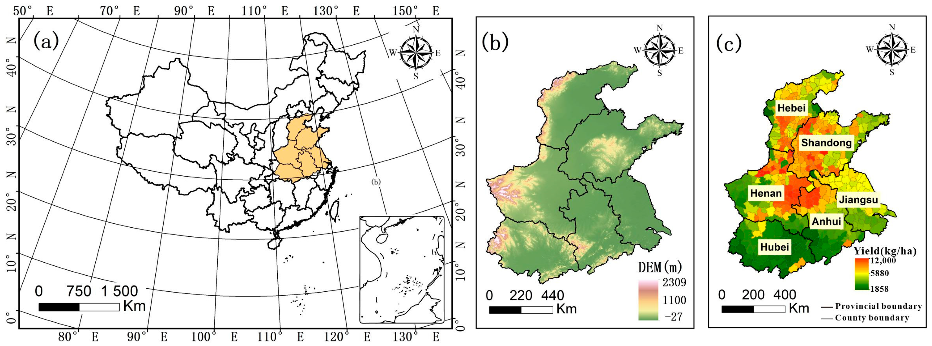
2.1. Research Area

The main winter wheat production areas in China (110°36′–122°11′ E, 29°4′–41°10′ N) include six provinces: Hebei, Shandong, Henan, Anhui, Jiangsu, and Hubei (Figure 1a) [16]. The climate is diverse and includes temperate continental monsoon climate, warm temperate monsoon climate, East Asian monsoon climate, warm temperate semihumid monsoon climate and subtropical humid monsoon climate zones, with rain and heat occurring during the same season [17]. In regard to the annual precipitation, except for Hebei Province that occurs within the 500 mm range, the other provinces occur within the 1000 mm range. The landforms include plains, hills, and mountains, with significant differences in altitude between east and west, with the highest elevation reaching 2309 m and the lowest elevation reaching −27 m (Figure 1b). The regional yield exhibits agglomeration characteristics. The areas with higher yields are concentrated in southern Hebei Province, western Shandong Province, eastern Henan Province, and northern Anhui Province, i.e., the central part of the Huanghuai Plain, while the areas with lower yields occur in the southern and western parts of the research area at higher elevations.

2.2. Data Description

To improve the modeling efficiency and reduce the difficulty of obtaining regional modeling data, meteorological data, soil data, terrain data and vegetation index data were selected for model construction in this research (Table 1). According to the spatial and temporal scopes (2014–2019), the data description and processing steps are as follows: (1) to ensure that the satellite images better reflect crop growth, Sentinel-2 satellite image data were screened in the Google Earth Engine by using a cloud coverage of 10% as the threshold. The NDVI was calculated by the monthly median synthesis method to obtain high-quality images for each month, that is, the median of each pixel time series NDVI value represents the month value; (2) the time-series daily soil moisture dataset was based on the soil moisture observed provided by China Meteorological Administration, and the accuracy was verified [18]. We calculated the mean data for March, April, and May each year; (3) mask extraction was performed based on the spatial production allocation model’s wheat planting area to ensure that the raster data needed for modeling all originated from wheat planting regions [19]. (4) With the use of the zonal statistics tool in ArcGIS, the county-level administrative unit was employed as the basic spatial unit. The raster data were subjected to mean statistical analysis, and the UpdateCursor tool in ArcGIS was used to assign yield data as attribute data to the corresponding spatial units. (5) Finally, the attribute table of the vector data was exported, with the environmental data as feature variables and the statistical yield as the target variable, to build the training data needed for the RF model.

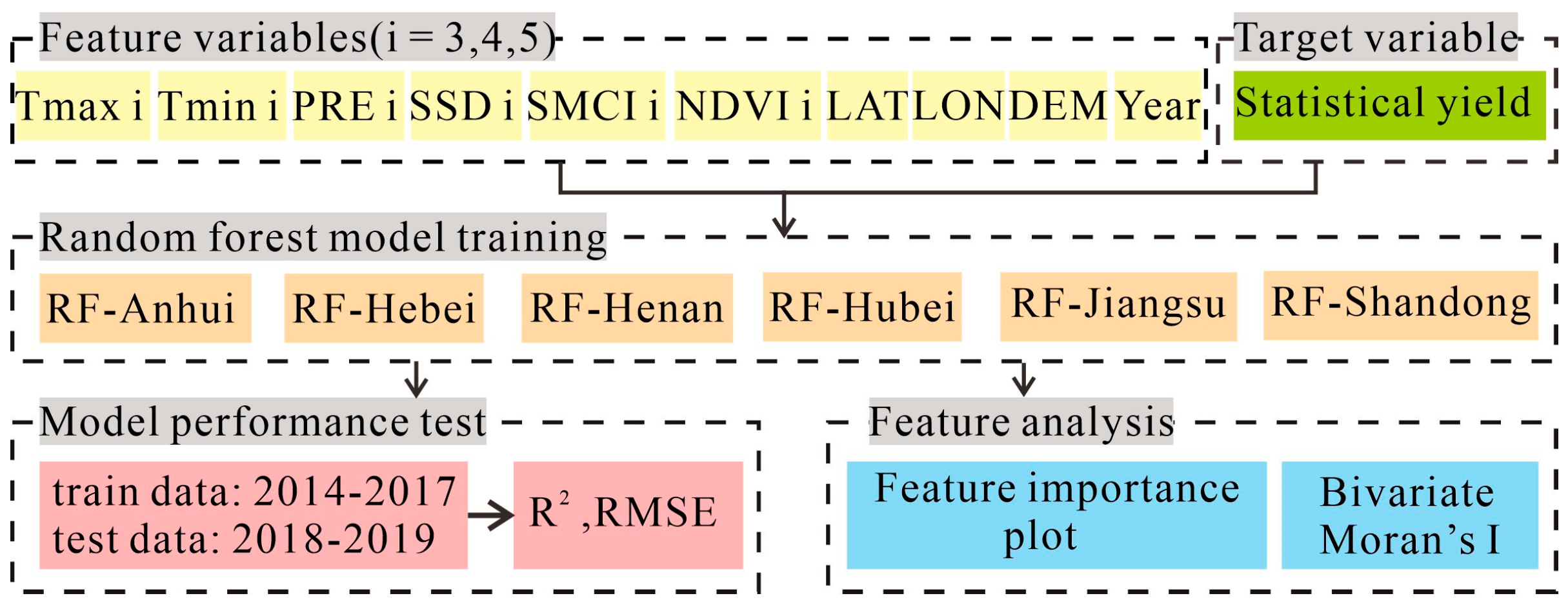
2.3. Analysis Workflow

Technical workflow as shown in Figure 2 mainly included the following steps: (1) The meteorological data, soil moisture data and vegetation index data during the critical growth periods of wheat (March, April, and May) were selected, and the year was used to represent the yield change due to the implementation of production management measures, variety updating and climate change as a feature variable [9,10], and the statistical yield was used as the target variable. (2) The data for 2018 and 2019 were used as validation data, and the data for the other years were used as training data [15]. An RF model for yield prediction was established for each province within the research area, and the model accuracy was evaluated using the coefficient of determination (R2) and root mean square error (RMSE). (3) These two feature analysis methods were used to explain the influence of key variables on the yield. First, RF partial dependence plots were conducted to obtain the nonlinear curve between the key variables and the output. Second, bivariate Moran’s I was employed to verify the spatial correlation between the key variables and the statistical yield.

2.4. Random Forest

The RF algorithm is an ensemble learning method developed by Breiman based on the combination of many decision trees [20]. Each tree is trained by selecting a random variable set and random samples from the training dataset. In each tree, approximately one-third of the cases, referred to as the out-of-bag (OOB) data, can be used to estimate the generalization error. The RF model can be used for both classification and regression purposes. If predictions are made by a classification algorithm, the final class will be the class with the most votes from all the decision trees. If a regression algorithm is used, the arithmetic mean of the regression results obtained by all the decision trees will be the final model output. The use of the RF model can improve the prediction accuracy with low computational complexity, and it is insensitive to multicollinearity of variables; moreover, the prediction results are robust to both missing and unbalanced data, and this model can be used to effectively predict the roles of up to thousands of explanatory variables [21]. In addition, the RF model contains a built-in variable importance measure and partial dependence, which can be used to visualize the functional form between the predictor variables and target variables, allowing users to investigate linear and nonlinear responses. The year was adopted as a numerical variable in this research, but in machine learning, the value of the year should not be a continuous variable but rather a categorical variable. Therefore, one-hot encoding was applied to convert the year variable [1,22].

2.5. Bivariate Moran’s I

Bivariate spatial autocorrelation analysis based on spatial statistics theory can provide measures of the spatial distribution pattern of two variables, namely, similarity and correlation, among geographic locations. Spatial correlation exists when two variables exhibit the same intensity and direction of change with the change in spatial location. If the spatial structures of the two variables significantly differ, they are spatially uncorrelated or exhibit a weak spatial correlation. In this research, Moran’s I was chosen as the bivariate spatial autocorrelation indicator. The calculation result depends on the difference between the variables and the relationship between the spatial locations. The value ranges from −1 to 1, and a positive value indicates a positive correlation. Conversely, a negative value indicates a negative correlation, while a value close to 0 indicates no correlation [23,24]. Bivariate Moran’s I can be calculated as follows:
I k l = Z k i j = 1 n W i j Z l j
Z k i = X k i X ¯ k σ k
Z l i = X l i X ¯ l σ l
where X k i is the value of variable k at position i , X l i is the value of variable l at position i , X k ¯ and X l ¯ are the mean values of variables k and l , respectively, σ k and σ l are the variances in variables k and l , respectively, and W i j is the spatial adjacency weight matrix.

3. Results and Discussion

3.1. Descriptive Statistics

A box plot was created to show the distributions of the extreme and mean values of the county-level statistical yield in each province in a specific year (Figure 3). Results showed that there were gaps in the distributions of the county-level statistical yields in the different provinces, and the yield gap was consistent among the different years. The yield variation at the county level in Anhui Province was relatively high. Notably, the variation ranges from 2014 to 2019 were 5964, 5919, 5739, 6949, 5322, and 5665 kg/ha. The county-level yield variation in Jiangsu Province was relatively low, with ranges from 2014 to 2019 of 4004, 3831, 3782, 3312, 3450 and 3952 kg/ha, respectively. The two provinces with the highest mean values were Henan Province and Shandong Province, with a stable value of approximately 6200 kg/ha. Moreover, the value in Jiangsu Province was approximately 5600 kg/ha, while Hubei Province exhibited the lowest value, at approximately 3600 kg/ha.

3.2. Model Performance Evaluation

The RF model has been demonstrated to provide a high modeling accuracy in relevant studies, so in this research, horizontal comparisons of different modeling methods were not conducted [1,25,26]. According to the division of the wheat growth period based on the BBCH scale, the time ranges of the feature variables selected in this research included key growth periods, such as tillering, booting, and flowering, which are closely related to the yield [7,27]. Then, we used the county-level administrative region of each province as the basic spatial unit in modeling and established an RF yield prediction model for each province. Then, the key environmental variables in each province were analyzed, and bivariate Moran’s I was adopted from a geospatial distribution perspective. The spatial correlations between the yield and environmental variables and between the environmental variables and the latitude and longitude were analyzed to determine the commonalities and differences in the relationships between the yield and environmental elements among the various provinces.
Results between statistical yield and predicted yield showed that the RF models exhibited a suitable fitting effect in 2018 and 2019 (Figure 4). The RMSE values of previous winter wheat yield models ranged from 600 to 900 kg/ha, but the R2 values were all approximately 0.9 [11,28]. In this research, the RMSE values of the various province-specific models varied between 200 and 650 kg/ha, remaining at a moderate level, while R2 was also maintained above 0.5. Among them, the RMSEs of the models for Henan, Hebei, and Jiangsu were smaller, which may be attributed to their larger winter wheat planting area and flatter terrain. The RMSE reached a minimum of 230 kg/ha in Jiangsu Province and a maximum of 640 kg/ha in Shandong Province (Figure 4e,l).
Compared with the RMSE of the RF-simulated yield at the county level, the accuracy of the provincial mean simulation results was greater, and the variation trend of the absolute difference in the regional mean between the different years remained consistent (Table 2). This may occur because the yields in some counties within the provincial area increased, while the yields decreased in other counties. These two effects offset each other, resulting in slight changes in the regional mean. Most absolute differences were below 300 kg/ha. The absolute difference in Jiangsu Province was the smallest in 2018, at 36.9 kg/ha, while the absolute difference in Anhui Province in 2018 was 270.4 kg/ha.

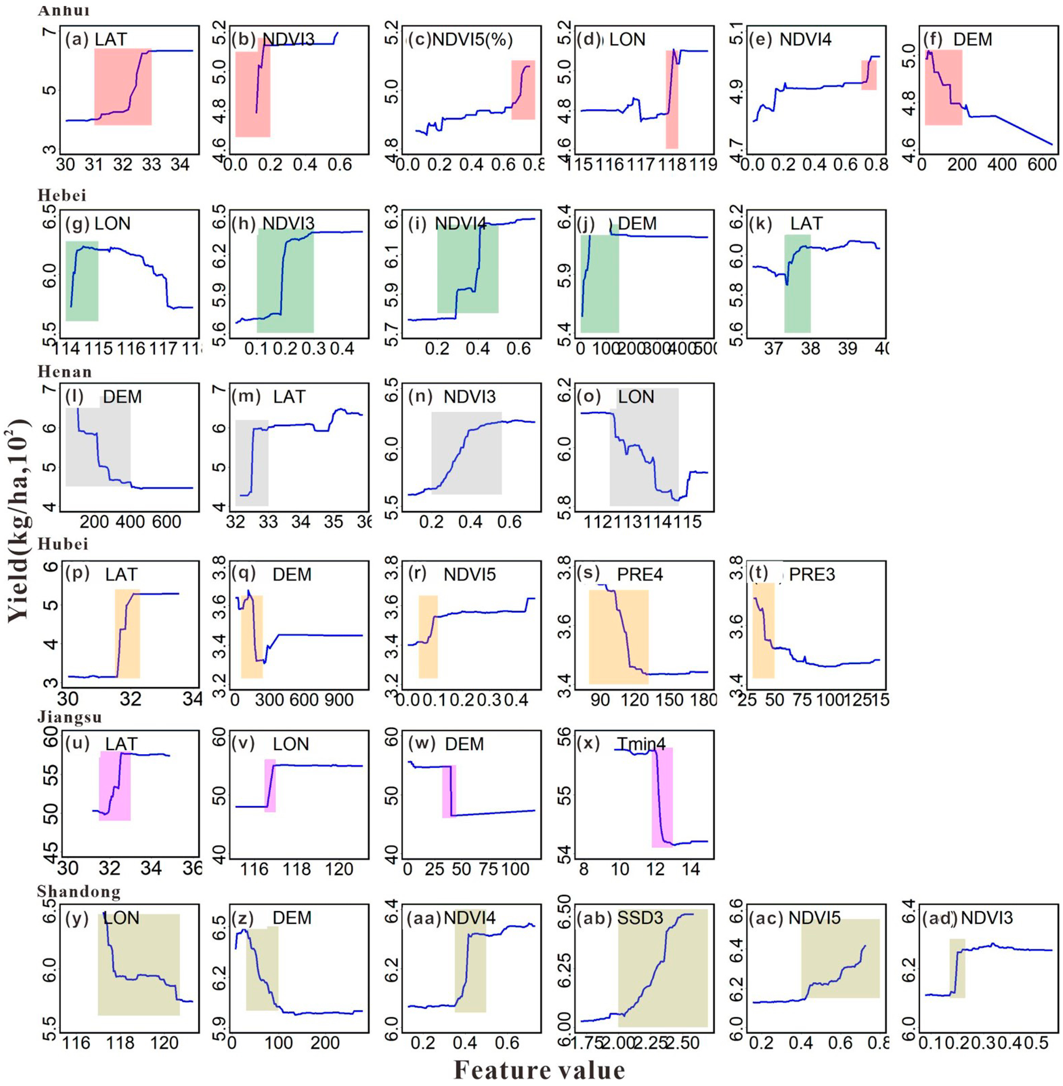
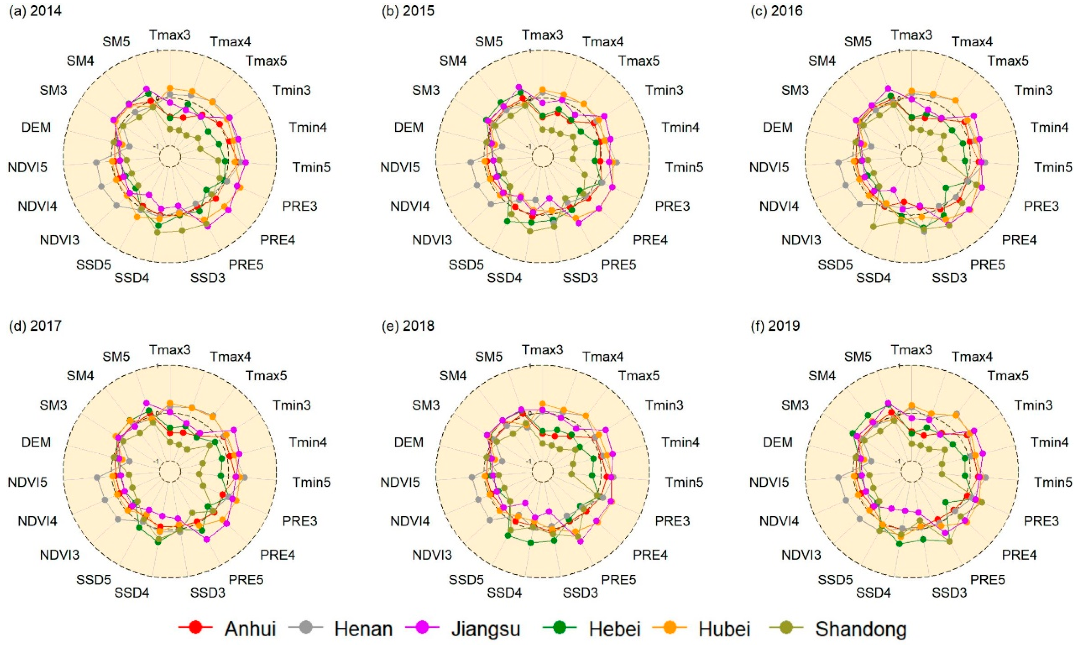
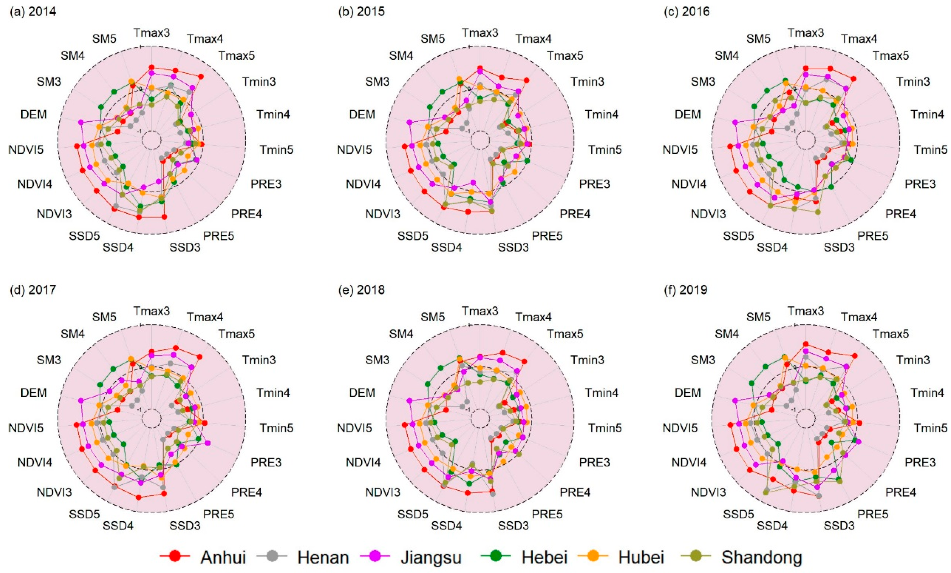
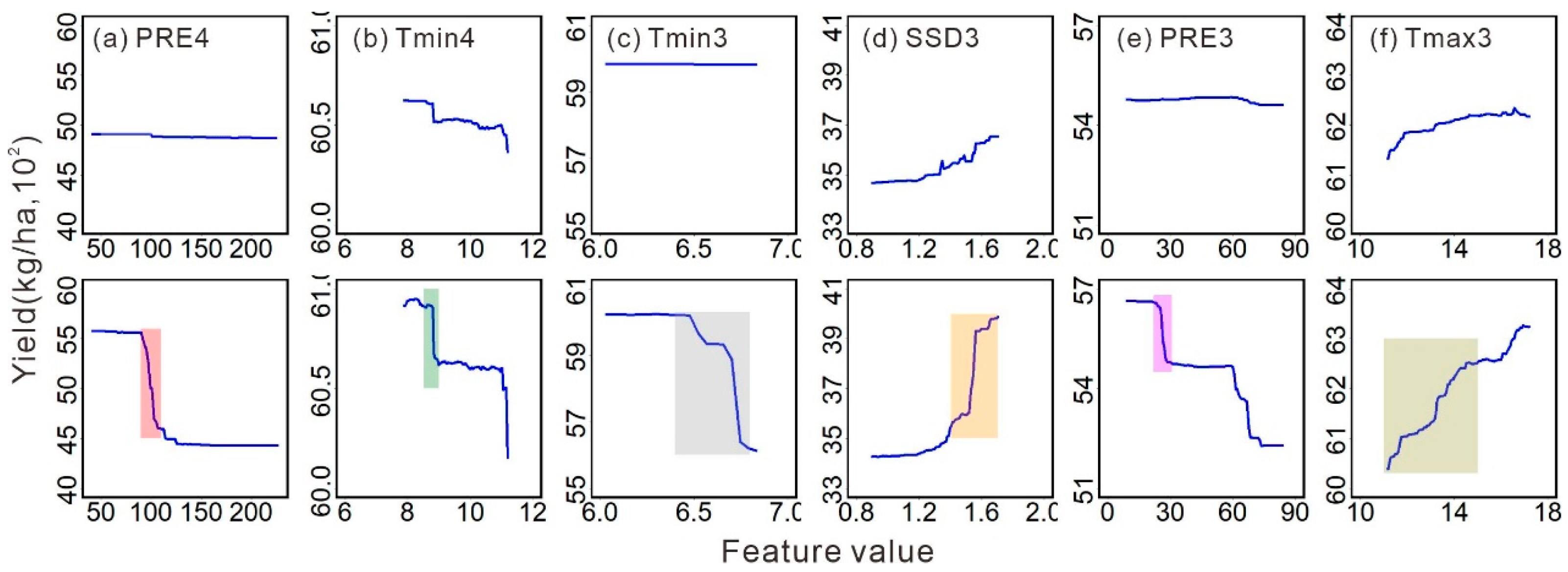
3.3. Variable Importance

Through variable importance analysis of the yield forecast model, the contribution of each variable to the model prediction results can be quantified, and the threshold range within which the variable significantly impacts the model results can be determined to select key variables for modeling, thus helping to improve the model calculation performance, reduce overfitting and enhance the model interpretability [5]. In this research, the feature variables with a yield influence degree greater than 200 kg/ha were mapped. The results showed that there was an obvious nonlinear relationship between the feature variables and yield, and all the feature variables exhibited threshold values. Beyond the threshold value, the yield variation remained stable.
The descriptive statistics of the yield showed that the yield in each province did not significantly change in the six years (Figure 3). Therefore, compared to the time range in previous studies, namely, more than 50 years, the yield gradually increased over time [5]. The year variable did not generate a significant effect in this research. Because light and temperature conditions are greatly affected by the spatial location and topographic characteristics on large scales, the latitude, longitude and DEM more notably impacted the yield prediction results for most provinces (Figure 5), and the DEM were already reported to have influence on long-term yield effects, that can be explored in determining yield classes and delineating yield stability zones [1]. While there was no significant relationship between soil water and yield, which may occur because the agricultural infrastructure is relatively complete, and the irrigation conditions are very mature affected by human activities. However, previous studies on farm-scale crop yield prediction and soil indices including brightness index and redness index have a certain correlation with yield [1,9]. Because the soil samples were expensive and also because the values do not vary substantially over relatively short periods of time, it is usually difficult to use temporal soil data for analysis in research [9].
The yield at the county level was not randomly distributed spatially but demonstrated spatial heterogeneity and agglomeration characteristics. For example, in the western Shandong Province, the yield in the east was low. Therefore, with increasing longitude, the yield in Shandong Province decreased from 6500 to 5500 kg/ha (Figure 5y). The yield in the northern part of Anhui Province was greater than that in the southern part. Therefore, with increasing latitude, the yield increased from 4000 to approximately 6100 kg/ha (Figure 5a). First, the slope, aspect, and altitude characteristics of the terrain affect the spatial distribution of illumination and temperature conditions. Second, hilly and mountainous areas are generally fragmented, the spatial resolution of the input data is low, and the mixed-pixel phenomenon is severe. The RMSE of the provincial yield forecast model was large (Figure 4a,d,f) [29]. In related studies, the topography was also used as a key variable in the analysis of scale and zonal effects and in simulation correction of the light-temperature potential yield and yield difference in crop yield prediction [30]. The topography affects the transfer of soil water and nutrients under gravity, especially on small scales such as field parcels, which is a factor that must be considered in field management zoning [31,32]. However, the spatial scale in this research was relatively large, and soil water imposed almost no effect on the yield.
Since crop dry matter accumulation results from photosynthetically active radiation, there is a significant correlation between the sunshine hours and yield [33]. Crops are affected to varying degrees by the temperature during different growth periods. An increase in the temperature at the early stage of the growth period could help wheat growth. For example, in Shandong Province, when the sunshine duration was more than 2 h in March, the yield gradually increased (Figure 5a,b), but very high temperatures could lead to vigorous growth. In April, the temperature at the peak growth stage was very high, accompanied by extreme climatic phenomena such as hot and dry winds, which reduced the growth period of wheat, affected grain filling, and eventually led to a decrease in the yield (Figure 5x) [26,34,35]. In addition, wind speed and relative humidity were also proved to have better relative importance for wheat yield prediction [26].
Previous studies have shown that better grain yield prediction results can be obtained by choosing variables that most directly relate to yield, such as biomass [7]. In this study, the NDVI can effectively indicate the growth and health status of crops, and higher values indicate crops that contain a higher concentration of chlorophyll, which is closely correlated with biomass [1,27]. However, the early and late stages of crop growth do not have a good response toward vegetation indices due to the low reflection, and it is different from the previous work that used the mean of the whole crop NDVI value [26]. In our study, it is important to use data from the critical growth period for predicting crop yields before harvesting. All provinces showed that the higher the NDVI value was, the greater the yield. Consistent with previous results, the peak values of the wheat NDVI were approximately 0.58, 0.80 and 0.88 in March, April and May, respectively (Figure 5) [27]. However, there was no significant relationship between the peak NDVI value and the yield. Therefore, after the NDVI3 reached 0.2 in the Anhui and Hebei Provinces and after the NDVI4 reached 0.4 in the Shandong Province, the yield stabilized with increasing NDVI. However, due to the saturation effect of the NDVI under the influence of a high vegetation cover, the sensitivity to vegetation growth was reduced, and a linear increase could not be achieved [36]. So, the vegetation index EVI should be incorporated into the modeling process in combination with other indices, because EVI has the ability to reduce the background canopy signal and enhance the high biomass reflection [26].

3.4. Bivariate Moran’s I

The conventional analysis methods aim to explore the statistical correlation among variables to explain the model. However, there is spatial continuity between the environmental variables and the statistical yield. Spatial continuity quantification via bivariate Moran’s I can be used to effectively identify spatial distribution patterns and spatial dependence between the yield and environmental variables and assess the strength and direction of correlations. This approach is currently widely used in environmental science and other fields to assess the strength and direction of correlations [23,24,37]. Since the NDVI can reflect the status of crop growth, there was a notable high–high spatial positive correlation between the yield and NDVI in the five provinces, i.e., areas with relatively high NDVI values exhibited relatively high winter wheat yields, and Moran’s I values were all greater than 0.7 (Figure 6). In provinces at higher latitudes, including Hebei, Henan, and Shandong, there was a weaker high–high spatial correlation between the yield and temperature and a high–low spatial negative correlation between the latitude and temperature. Notably, the lower the latitude and the higher the temperature were, the greater the yield. In this research, in Anhui Province located at a lower latitude, there was a significantly negative high–low spatial correlation between the yield and precipitation, while a significant positive spatial correlation was observed between the yield and sunshine hours.
However, bivariate spatial autocorrelation can only provide a measure of the strength of spatial relationships but cannot reflect causal relationships, namely, it cannot explain why yield changes are caused by changes in environmental variables; additionally, bivariate spatial autocorrelation is sensitive to spatial scale effects [38,39]. In this research, within the provincial spatial range, the relationships between the meteorological conditions, NDVI and yield were high, while the relationships between the soil water content and yield were almost nonexistent. However, in precision management zoning studies at the field parcel scale, the spatial distribution of meteorological elements is uniform, and soil water and nutrients are the main causes of yield differences [40,41]. Therefore, the determination of feature variables at different spatial scales should consider the joint influence of the above factors. It is necessary to further determine the yield-limiting factors according to the influences of agronomic management measures and economic and social factors.
The yield changes caused by the latitude and longitude were mainly due to the effects of these factors on the spatial distributions of sunshine hours, temperature, and precipitation. Therefore, the longitude and latitude were identified as key variables in the yield simulation process (Figure 5). To illustrate the relationships between the environmental variables and latitude and longitude in regional wheat yield simulations, bivariate Moran’s I analysis was also conducted in this research. The results showed that the temperature and longitude in Shandong Province exhibited a significant negative spatial correlation, and for bivariate Moran’s I, the absolute values were all above 0.5, i.e., the maximum temperature gradually increased away from the coastline, and the decadal trends remained the same. The bivariate Moran’s I index values between the longitude and environmental variables such as precipitation and soil moisture in the inland provinces were all approximately 0, indicating no significant spatial correlation (Figure 7a–f).
Previous research has indicated that the longitude mainly causes changes in environmental elements by affecting the distributions of land and sea, while changes in the solar radiation due to latitude lead to longitudinal zone changes in heat, also referred to as longitudinal zonality [42,43]. In this research, the absolute values of bivariate Moran’s I between most environmental variables, such as temperature, precipitation, and sunshine hours, and latitude were greater than 0.5 (Figure 8). Precipitation and latitude showed a negative spatial correlation, i.e., areas at higher latitudes exhibited less precipitation, and conversely, the number of sunshine hours was greater. This was obvious in the Anhui Province, which occurs in a transitional area between the warm temperate zone and the subtropical zone. However, relying solely on spatial variability is insufficient for understanding the relationship between environmental variables and spatial location, the temporal variability should also be taken into account [1].
To verify the effects of the longitude, latitude and environmental variables on the yield modeling results, variable importance analysis was again conducted after the longitude and latitude were removed. The results showed that the impact of non-critical variables on the yield significantly increased. Choosing rainfall in the Anhui Province in April as an example, after excluding the latitude and longitude, as rainfall increased from 100 to 120 mm, the yield decreased by approximately 1000 kg/ha (Figure 9a). However, before the deletion of latitude and longitude, the precipitation in April imposed almost no effect on the yield, and the other provinces showed similar phenomena. This may occur because the spatial location generates a certain substitution effect on environmental variables, thus masking the effects of environmental variables such as temperature, precipitation, and sunshine on the yield in modeling. This phenomenon is more obvious in more notable zoned regions. Therefore, previous studies have used permutation importance, lasso regularisation, ridge regularisation, tree-based selection, boruta, and recursive feature elimination methods to minimize the risk of missing relevant predictors [9]. Despite the advantage of insensitivity of the RF model in complex data structures, the influence of variable collinearity should be considered in detecting the hidden non-linear relationships among all variables. And it is necessary to analyze the significant correlations between individual environmental indicators and response variables to maintain the optimum range of values, and to prevent stresses at different stages of crop growth [26].

3.5. Limitations of This Research

In this research, the county-level administrative districts in the provinces were used as the basic spatial units to establish a wheat yield prediction model. Through variable importance analysis and bivariate Moran’s I, the relationships between the variables and yield could be visualized from two perspectives: attributes and space. This research provides important reference data for understanding the potential of light, temperature and precipitation resources in different regions, improving the utilization rate of light energy, as well as the need to adjust the planting layout and the selection and breeding of new varieties. However, the following influencing factors were not considered. An extreme climate is the main reason for drastic changes in the yield, so extreme climate indicators and multiple future climate scenarios derived from meteorological data are important for research on the occurrence patterns of climate extremes in time and space, the development of key areas for climate monitoring and prevention, and the improvement in farmland infrastructure to reduce the potential threat to yields [44,45]; however, this requires the support of hourly meteorological monitoring data with higher temporal resolution. In addition, due to data collection difficulties in terms of the regional chemical fertilizer application amount, total power of agricultural machinery, and rural labor input [46], the effect of agricultural factor inputs on the yield was not considered herein. In addition, from a county-level application perspective, on the basis of accurate parcel identification, meteorological stations and soil stations combined with accurate yield measurement data of agricultural machinery were used to accurately reflect the crop planting environment, rather than the data with errors obtained by regional interpolation methods, so as to realize crop yield estimation and regional yield mapping at pixel scale and farm scale [1,47], which is an important direction of future research.

4. Conclusions

In this research, the RF model was used to establish a winter wheat yield prediction model. The model for each province exhibited favorable accuracy. The key variables in each province were identified via RF variable importance mapping. Notably, the longitude, latitude, and DEM were key variables in all provinces. The NDVI was a key variable in Anhui, Henan, Jiangsu, and Shandong; rainfall in March and April was a key variable in Hebei Province located at higher latitudes, and Hubei Province exhibited the lowest temperature in April. The bivariate Moran’s I results showed that the NDVI and yield exhibited high positive spatial correlations, while the temperature, precipitation, and sunshine hours exhibited notable zonal characteristics. Thus, environmental variables related to the spatial location should be considered in the modeling process.

Author Contributions

Conceptualization, H.X. and H.Y.; methodology, H.X. and H.Y.; software, H.X., B.W., Y.L. and L.J.; validation, Y.L. and B.W.; writing—original draft preparation, H.X., H.Y. and L.J.; writing—review and editing, Z.Z. and X.Z.; visualization, H.S., L.J. and S.W.; funding acquisition, H.X. All authors have read and agreed to the published version of the manuscript.

Funding

This research was funded by the Natural Science Foundation of Shandong Province, grant number ZR2021QC183.

Data Availability Statement

The data are not publicly available due to privacy or ethical restrictions.

Conflicts of Interest

The authors declare no conflicts of interest.

References

  1. Sunoj, S.; Polson, B.; Vaish, I.; Marcaida, M., III; Longchamps, L.; van Aardt, J.; Ketterings, Q.M. Corn grain and silage yield class prediction for zone delineation using high-resolution satellite imagery. Agric. Syst. 2024, 218, 104009. [Google Scholar] [CrossRef]
  2. Gang, Z.; Siebert, S.; Enders, A.; Rezaei, E.E.; Yan, C.; Ewert, F. Demand for multi-scale weather data for regional crop modeling. Agric. For. Meteorol. 2015, 200, 156–171. [Google Scholar] [CrossRef]
  3. Dilli, P.; Boogaard, H.; de Wit, A.; van der Velde, M.; Claverie, M.; Nisini, L.; Janssen, S.; Osinga, S.; Athanasiadis, I.N. Machine learning for regional crop yield forecasting in Europe. Field Crops Res. 2022, 276, 108377. [Google Scholar] [CrossRef]
  4. Ryoya, T.; Matsui, T.; Tanaka, T.S.T. Winter wheat yield prediction using convolutional neural networks and UAV-based multispectral imagery. Field Crops Res. 2023, 291, 108786. [Google Scholar] [CrossRef]
  5. Rosenzweig, C.; Elliott, J.; Deryng, D.; Ruane, A.C.; Müller, C.; Arneth, A.; Boote, K.J.; Folberth, C.; Glotter, M.; Khabarov, N.; et al. Assessing agricultural risks of climate change in the 21st century in a global gridded crop model intercomparison. Proc. Natl. Acad. Sci. USA 2014, 11, 3268–3273. [Google Scholar] [CrossRef] [PubMed]
  6. Yi, X. Combining CERES-Wheat model, Sentinel-2 data, and deep learning method for winter wheat yield estimation. Int. J. Remote Sens. 2022, 43, 630–648. [Google Scholar] [CrossRef]
  7. Zare, H.; Weber, T.K.D.; Ingwersen, J.; Nowak, W.; Gayler, S.; Streck, T. Within-season crop yield prediction by a multi-model ensemble with integrated data assimilation. Field Crops Res. 2024, 308, 109293. [Google Scholar] [CrossRef]
  8. Wei, L.; Yang, H.; Niu, Y.; Zhang, Y.; Xu, L.; Chai, X. Wheat biomass, yield, and straw-grain ratio estimation from multi-temporal UAV-based RGB and multispectral images. Biosyst. Eng. 2023, 234, 187–205. [Google Scholar] [CrossRef]
  9. Bansal, Y.; Lillis, D.; Kechadi, M.T. A neural meta model for predicting winter wheat crop yield. Mach. Learn. 2024, 113, 3771–3788. [Google Scholar] [CrossRef]
  10. Hoffman, A.L.; Kemanian, A.R.; Forest, C.E. Analysis of climate signals in the crop yield record of sub-Saharan Africa. Glob. Chang. Biol. 2018, 24, 143–157. [Google Scholar] [CrossRef]
  11. Li, L.; Wang, B.; Feng, P.; Wang, H.; He, Q.; Wang, Y.; Liu, D.L.; Li, Y.; He, J.; Feng, H.; et al. Crop yield forecasting and associated optimum lead time analysis based on multi-source environmental data across China. Agric. For. Meteorol. 2021, 308, 108558. [Google Scholar] [CrossRef]
  12. Karsoliya, S. Approximating number of hidden layer neurons in multiple hidden layer BPNN architecture. Int. J. Eng. Trends Technol. 2012, 3, 714–717. [Google Scholar]
  13. El-Sharkawy, M.; Li, J.; Kamal, N.; Mahmoud, E.; Omara, A.E.-D.; Du, D. Assessing and Predicting Soil Quality in Heavy Metal-Contaminated Soils: Statistical and ANN-Based Techniques. J. Soil. Sci. Plant Nutr. 2023, 23, 6510–6526. [Google Scholar] [CrossRef]
  14. Barlow, K.M.; Christy, B.P.; O’Leary, G.J.; Riffkin, P.A.; Nuttall, J.G. Simulating the impact of extreme heat and frost events on wheat crop production: A review. Field Crops Res. 2015, 171, 109–119. [Google Scholar] [CrossRef]
  15. Yang, H.S.; Bishop, T.F.A.; Filippi, P. Data-driven, early-season forecasts of block sugarcane yield for precision agriculture. Field Crops Res. 2022, 276, 108360. [Google Scholar] [CrossRef]
  16. Xu, H.; Huang, F.; Zuo, W.; Tian, Y.; Zhu, Y.; Cao, W.; Zhang, X. Impacts of spatial zonation schemes on yield potential estimates at the regional scale. Agronomy 2020, 10, 631. [Google Scholar] [CrossRef]
  17. Zheng, J.; Yin, Y.H.; Li, B.Y. A new scheme for climate regionalization in China. Acta Geogr. Sin. 2010, 65, 3–12. [Google Scholar] [CrossRef]
  18. Li, Q.; Shi, G.; Shangguan, W.; Nourani, V.; Li, J.; Li, L.; Huang, F.; Zhang, Y.; Wang, C.; Wang, D.; et al. A 1 km daily soil moisture dataset over China using in situ measurement and machine learning. Earth Syst. Sci. Data 2022, 14, 5267–5286. [Google Scholar] [CrossRef]
  19. International Food Policy Research Institute (IFPRI). Global Spatially-Disaggregated Crop Production Statistics Data for 2020 Version 1.0.0. Harvard Dataverse, V1. Available online: https://www.agrodep.org/resource/harvestchoice-spatial-production-allocation-model-spam-2000 (accessed on 19 December 2023).
  20. Breiman, L. Random forests. Mach. Learn. 2001, 45, 5–32. [Google Scholar] [CrossRef]
  21. Elbeltagi, A.; Srivastava, A.; Deng, J.; Li, Z.; Raza, A.; Khadke, L.; Yu, Z.; El-Rawy, M. Forecasting vapor pressure deficit for agricultural water management using machine learning in semi-arid environments. Agric. Water Manag. 2023, 283, 108302. [Google Scholar] [CrossRef]
  22. Pedregosa, F.; Varoquaux, G.; Gramfort, A.; Michel, V.; Thirion, B.; Grisel, O.; Blondel, M.; Prettenhofer, P.; Weiss, R.; Dubourg, V.; et al. Scikit-learn: Machine learning in Python. J. Mach. Learn. Res. 2011, 12, 2825–2830. [Google Scholar]
  23. Lee, S.-I. Developing a bivariate spatial association measure: An integration of Pearson’s r and Moran’s I. J. Geogr. Syst. 2001, 3, 369–385. [Google Scholar] [CrossRef]
  24. Hu, B.; Shao, S.; Ni, H.; Fu, Z.; Huang, M.; Chen, Q.; Shi, Z. Assessment of potentially toxic element pollution in soils and related health risks in 271 cities across China. Environ. Pollut. 2021, 270, 116196. [Google Scholar] [CrossRef] [PubMed]
  25. Xu, H.; Zhang, X.; Ye, Z.; Jiang, L.; Qiu, X.; Tian, Y.; Zhu, Y.; Cao, W. Machine learning approaches can reduce environmental data requirements for regional yield potential simulation. Eur. J. Agron. 2021, 129, 126335. [Google Scholar] [CrossRef]
  26. Arshad, S.; Kazmi, J.H.; Javed, M.G.; Mohammed, S. Applicability of machine learning techniques in predicting wheat yield based on remote sensing and climate data in Pakistan, South Asia. Eur. J. Agron. 2023, 147, 126837. [Google Scholar] [CrossRef]
  27. Narin, M.G.; Noyan, M.F.; Abdikan, S. Monitoring Vegetative Stages of Sunflower and Wheat Crops with Sentinel-2 Images According to BBCH-Scale. J. Agric. Fac. Gaziosmanpasa Univ. 2021, 38, 46–52. [Google Scholar] [CrossRef]
  28. Cao, J.; Zhang, Z.; Luo, Y.; Zhang, L.; Zhang, J.; Li, Z.; Tao, F. Wheat yield predictions at a county and field scale with deep learning, machine learning, and google earth engine. Eur. J. Agron. 2021, 123, 126204. [Google Scholar] [CrossRef]
  29. Wei, J.; Tang, X.; Gu, Q.; Wang, M.; Ma, M.; Han, X. Using solar-induced chlorophyll fluorescence observed by OCO-2 to predict autumn crop production in China. Remote Sens. 2019, 11, 1715. [Google Scholar] [CrossRef]
  30. Leo, S.; De Antoni Migliorati, M.; Grace, P.R. Predicting within-field cotton yields using publicly available datasets and machine learning. Agron. J. 2021, 113, 1150–1163. [Google Scholar] [CrossRef]
  31. Tziachris, P.; Aschonitis, V.; Chatzistathis, T.; Papadopoulou, M. Assessment of spatial hybrid methods for predicting soil organic matter using DEM derivatives and soil parameters. CATENA 2019, 174, 206–216. [Google Scholar] [CrossRef]
  32. Fridgen, J.J.; Kitchen, N.R.; Sudduth, K.A.; Drummond, S.T.; Wiebold, W.J.; Fraisse, C.W. Management zone analyst (MZA) software for subfield management zone delineation. Agron. J. 2004, 96, 100–108. [Google Scholar] [CrossRef]
  33. Mu, H.; Jiang, D.; Wollenweber, B.; Dai, T.; Jing, Q.; Cao, W. Long-term low radiation decreases leaf photosynthesis, photochemical efficiency and grain yield in winter wheat. J. Agron. Crop Sci. 2010, 196, 38–47. [Google Scholar] [CrossRef]
  34. You, L.; Rosegrant, M.W.; Wood, S.; Sun, D. Impact of growing season temperature on wheat productivity in China. Agric. For. Meteorol. 2009, 149, 1009–1014. [Google Scholar] [CrossRef]
  35. Liu, B.; Liu, L.; Tian, L.; Cao, W.; Zhu, Y.; Asseng, S. Post-heading heat stress and yield impact in winter wheat of China. Glob. Chang. Biol. 2014, 20, 372–381. [Google Scholar] [CrossRef]
  36. Coyne, P.I.; Aiken, R.M.; Maas, S.J.; Lamm, F.R. Evaluating YieldTracker forecasts for maize in western Kansas. Agron. J. 2009, 101, 671–680. [Google Scholar] [CrossRef]
  37. Jia, X.; Hu, B.; Marchant, B.P.; Zhou, L.; Shi, Z.; Zhu, Y. A methodological framework for identifying potential sources of soil heavy metal pollution based on machine learning: A case study in the Yangtze Delta, China. Environ. Pollut. 2019, 250, 601–609. [Google Scholar] [CrossRef] [PubMed]
  38. Tiefelsdorf, M. Some practical applications of Moran’s I’s exact conditional distribution. Pap. Reg. Sci. 1998, 77, 101–129. [Google Scholar] [CrossRef]
  39. Tiefelsdorf, M.; Boots, B. A note on the extremities of local Moran’s Iis and their impact on global Moran’s I. Geogr. Anal. 1997, 29, 248–257. [Google Scholar] [CrossRef]
  40. Zhang, X.; Jiang, L.; Qiu, X.; Qiu, J.; Wang, J.; Zhu, Y. An improved method of delineating rectangular management zones using a semivariogram-based technique. Comput. Electron. Agric. 2016, 121, 74–83. [Google Scholar] [CrossRef]
  41. Albornoz, V.M.; Cid-García, N.M.; Ortega, R.; Ríos-Solís, Y.A. A hierarchical planning scheme based on precision agriculture. In Handbook of Operations Research in Agriculture and the Agri-Food Industry; Springer: New York, NY, USA, 2015; pp. 129–162. [Google Scholar] [CrossRef]
  42. Shao, J.; Li, Y.; Ni, J. The characteristics of temperature variability with terrain, latitude and longitude in Sichuan-Chongqing Region. J. Geogr. Sci. 2012, 22, 223–244. [Google Scholar] [CrossRef]
  43. Hopkins, J.W. Correlation of air temperature normals for the Canadian Great Plains with latitude, longitude, and altitude. Can. J. Earth Sci. 1968, 5, 199–210. [Google Scholar] [CrossRef]
  44. Zheng, Z.; Hoogenboom, G.; Cai, H.; Wang, Z. Winter wheat production on the Guanzhong Plain of Northwest China under projected future climate with SimCLIM. Agric. Water Manag. 2020, 239, 106233. [Google Scholar] [CrossRef]
  45. Raza, A.; Saber, K.; Hu, Y.; Ray, R.L.; Kaya, Y.Z.; Dehghanisanij, H.; Kisi, O.; Elbeltagi, A. Modelling reference evapotranspiration using principal component analysis and machine learning methods under different climatic environments. Irrig. Drain. 2023, 72, 945–970. [Google Scholar] [CrossRef]
  46. Yuan, W.; Liu, S.; Liu, W.; Zhao, S.; Dong, W.; Tao, F.; Chen, M.; Lin, H. Opportunistic market-driven regional shifts of crop practices reduce food production capacity of China. Earth’s Future 2018, 6, 634–642. [Google Scholar] [CrossRef]
  47. Perich, G.; Turkoglu, M.O.; Graf, L.V.; Wegner, J.D.; Aasen, H.; Walter, A.; Liebisch, F. Pixel-based yield map and prediction from Sentinel-2 using spectral indices and neural networks. Field Crops Res. 2023, 292, 108824. [Google Scholar] [CrossRef]
Figure 1. Research area: (a) geographical location, (b) DEM, and (c) spatial distribution of the mean statistical yield values (2014–2019) in the six provinces; for each color, the basic spatial unit is the county.
Agronomy 14 01623 g001
Figure 2. Analysis workflow. The index i indicates the months adopted in this research, with 3, 4 and 5 corresponding to March, April and May, respectively.
Agronomy 14 01623 g002
Figure 3. Box plot of the statistical yield. The upper line of the box is the maximum yield, the midline is the median yield, the lower line is the minimum yield, and the black triangle denotes an outlier.
Agronomy 14 01623 g003
Figure 4. Relationship between the statistical yield and RF-simulated yield.
Agronomy 14 01623 g004
Figure 5. As the feature variables changed and the yield variation exceeded 200 kg/ha, the partial dependence plots showed nonlinear relationships between the feature variables and yield.
Agronomy 14 01623 g005
Figure 6. Radar diagram of the bivariate Moran’s I values between the yield and the feature variables.
Agronomy 14 01623 g006
Figure 7. Radar diagram of the bivariate Moran’s I values between the longitude and environmental variables.
Agronomy 14 01623 g007
Figure 8. Radar diagram of the bivariate Moran’s I values between the latitude and environmental variables.
Agronomy 14 01623 g008
Figure 9. Changes in the nonlinear relationship between the environmental variables and yield using partial dependence plots before (upper) and after (lower) the deletion of the latitude and longitude.
Agronomy 14 01623 g009
Table 1. Description of the data needed in this research.
Data TypeElementFormatSourceTime ResolutionSpatial Resolution
Meteorological dataHighest temperature (Tmax), minimum temperature (Tmin), sunshine hours (SSD), and precipitation (PRE)tiffMeteorological Information Center of China Meteorological Administration (https://data.cma.cn/, accessed on 19 December 2023)Monthly1 km
Soil dataTen-cm soil surface moisturetiffA Big Earth Data Platform for Three Poles
(https://poles.tpdc.ac.cn/zh-hans/, accessed on 1 April 2023)
Daily1 km
Yield dataStatistical wheat yieldcsvChina Economic and Social Big Data Research Platform (data.cnki.net)YearlyCounty area
Remote sensing dataVisible light band and near-infrared bandtiffSentinel-2, Google Earth EngineMonthly, median composite10 m
Terrain dataDigital elevation model (DEM)tiffSRTMGL1_003 DEM (https://lpdaac.usgs.gov/products/srtmgl1v003/, accessed on 19 December 2023)/30 m
Other dataWheat planting areatiffSpatial production allocation model (SPAM) /10 km
Table 2. Absolute difference between the regional mean simulated by the RF model and the statistical yield mean in 2018 and 2019.
YearAbsolute Difference of the Regional Mean (kg/ha)
AnhuiHebeiHenanHubeiJiangsuShandong
2018270.4176.7209.968.236.986.5
201985.6225.512973.2142.9108.7
Disclaimer/Publisher’s Note: The statements, opinions and data contained in all publications are solely those of the individual author(s) and contributor(s) and not of MDPI and/or the editor(s). MDPI and/or the editor(s) disclaim responsibility for any injury to people or property resulting from any ideas, methods, instructions or products referred to in the content.

