Vegetation’s Dynamic Changes, Spatial Trends, and Responses to Drought in the Yellow River Basin, China

Abstract

Drought is a complex and recurrent natural disaster that can have devastating impacts on economies, societies, and ecosystems around the world. In light of climate change, the frequency, duration, and severity of drought events worldwide have increased, and extreme drought events have caused more severe and irreversible damage to terrestrial ecosystems. Therefore, estimating the resilience of different vegetation to drought events and vegetation’s response to damage is crucial to ensuring ecological security and guiding ecological restoration. Based on meteorological and remote-sensing datasets from 1982 to 2022, the spatial distribution characteristics and temporal variability of vegetation were identified in the Yellow River Basin (YRB), the dynamic changes and recurrence periods of typical drought events were clarified, and the driving effects of different drought types on vegetation were revealed. The results indicated that (1) during the research period, the standardized vegetation water-deficit index (SVWI) showed a downward trend in the YRB, with a 99.52% probability of abrupt seasonal changes in the SVWI occurring in January 2003; (2) the characteristic values of the grid trend Zs were −1.46 and 0.20 in winter and summer, respectively, indicating a significant downward trend in the winter SVWI; (3) the drought with the highest severity (6.48) occurred from September 1998 to February 1999, with a recurrence period of 8.54 years; and (4) the growth of vegetation was closely related to drought, and as the duration of drought increased, the sensitivity of vegetation to drought events gradually weakened. The research results provide a new perspective for identifying vegetation’s dynamic changes and responses to drought, which is of great significance in revealing the adaptability and potential influencing factors of vegetation in relation to climate.

1. Introduction

In a global context, the frequency, duration, and severity of future drought events are projected to significantly increase [1,2,3,4,5]. Drought events not only impact the distribution of water resources but may also alter eco-hydrological processes, affecting the normal vegetation growth and thus causing damage to ecosystems [6,7,8]. As a vital component of terrestrial ecosystems, vegetation is a key indicator of the energy transfer between land and atmosphere, ecosystem services, and the global energy cycle [9,10]. Specifically, there are significant differences in the resistance (i.e., sensitivity) of different types of vegetation to drought [11]. Due to the complexity of eco-hydrological processes, vegetation’s responses to drought exhibit spatiotemporal heterogeneity and lag effects [12,13]. Unlike meteorological and hydrological drought impacts on agriculture and water resources, vegetation is more sensitive to intense and prolonged drought events [14,15,16]. Therefore, exploring the escalating impacts of drought disasters on ecosystems, evaluating the drought response characteristics of different vegetation types, and formulating targeted measures are crucial to ensuring ecological security and sustaining ecosystem functions.

Precipitation serves as the primary water source for natural vegetation in arid and semi-arid regions, making the response of vegetation to meteorological drought a longstanding focal point in meteorology, hydrology, and ecology [17]. Vegetation, as a key indicator of environmental changes at various scales, has the ability to modify surface evapotranspiration, reflectivity, and roughness, playing a crucial role in energy exchange, carbon cycling, climate change, and hydrological processes [18,19,20]. Moreover, influenced by human activities and climate change, obvious alterations in hydrological characteristics have occurred, leading to severe degradation of the water resource availability for vegetation growth worldwide and consequently exacerbating the impacts of meteorological drought on vulnerable vegetation [21,22]. Traditional vegetation diagnosis methods mostly choose the best-fitting model, ignoring the uncertainty or error range of the model, which may make it difficult to effectively reflect the actual trends in time series changes. In this study, the Bayesian Estimator of Abrupt Seasonal and Trend Change Algorithm (BEAST) was used to aggregate many models into an average model and obtain the probability of change at any given time point through ensemble learning, thus clearly describing various uncertainties [23,24].

Terrestrial vegetation is a vital link in the global cycles of carbon, water, and energy [10,14,25]. Water availability permeates the entire growth process of vegetation and is one of the momentous environmental factors influencing vegetation, particularly in arid and semi-arid regions where vegetation growth is more water-limited [12]. Drought, as one of the most destructive natural disasters worldwide, has a major impact on the carbon sink function of terrestrial ecosystems, and is one of the crucial factors influencing vegetation changes on land [26,27]. Vegetation exhibits a high sensitivity to climate change, with its growth being strongly affected by drought. Under current global changes, mounting evidence suggests that the increasingly frequent drought events will significantly inhibit terrestrial vegetation growth, causing more severe, prolonged, and irreversible damage to terrestrial ecosystems [13,22,28,29]. The impact of meteorological drought on vegetation varies with factors such as the vegetation type and the duration of drought, with different regions and vegetation types having varying water requirements, exhibiting significant spatial heterogeneity [14,16]. Prolonged meteorological drought can lead to a sharp decline in vegetation’s water content, resulting in slow crop growth and reduced yields [30,31,32]. Therefore, clarifying the response characteristics of vegetation to meteorological drought in different regions is of great significance in relation to mitigating the impact of meteorological drought on vegetation systems and formulating drought-resistant strategies tailored to local conditions.

Temperature and precipitation are the most critical meteorological factors influencing ecological vegetation changes, which are also key indicators for constructing drought indices. For example, globally, temperature is the primary contributing factor to vegetation changes [33]. In the central part of the Eurasian continent, the growth of spring vegetation depends on the rapid increase in temperature, and during the growing season, it is mainly driven by precipitation [34]. Using the Standardized Precipitation Evapotranspiration Index (SPEI), Vicente-Serrano et al. analyzed the response characteristics of global vegetation to meteorological drought and found a close relationship between the vegetation response time and drought in 72% of vegetated areas globally [14]. Tietjen et al. suggested that the increased sensitivity of vegetation to precipitation could lead to higher ecosystem risks [35]. At the regional scale, the effects of temperature and precipitation on ecological vegetation vary [36]. Chu et al. found that vegetation in the northeastern part of Heilongjiang Province was mainly affected by precipitation during the growing season, with temperature being the crucial factor concerning vegetation changes during spring, and that vegetation exhibited a negative correlation with precipitation in autumn [37]. Nzabarinda et al. developed a simple linear regression model to predict future vegetation conditions in Africa, helping monitor and maintain ecosystem health by tracking changes in vegetation disturbance [38]. However, current research has little focus on vegetation feedback to drought processes in terrestrial systems, resulting in the majority of vegetation responses to drought in terrestrial systems being assessed using multivariate indices or vegetation remote-sensing indices, which make it difficult to directly reflect the actual dynamic balance of the water supply and demand for vegetation during drought processes [39,40]. Moreover, vegetation indices are susceptible to the influences of floods, pests, fires, and hailstorms, making them potentially suboptimal for reflecting vegetation drought stress [41]. It is necessary to construct an index that can simultaneously reflect meteorological and hydrological conditions, as well as the dynamic balance of the vegetation supply and demand for water, to monitor the response status of vegetation to drought [42].

The Yellow River Basin (YRB) spans the northern, eastern, central, and western geographical tiers of China, which is an important cluster area for ecological barriers [43]. In recent years, droughts have been frequent in the basin, with significant spatial heterogeneity in the vegetation distribution and varying responses of different vegetation types to drought [5,31,40]. Previous studies have mainly focused on meteorological or hydrological drought in the YRB, which may have overlooked the dynamic response of vegetation to drought [44,45]. With global warming, there has been an increase in the frequency of extreme climate events occurring in the YRB, exacerbating disaster losses and adversely affecting vegetation growth [46,47]. Therefore, investigating the relationship between extreme climate events and vegetation is important in terms of maintaining ecological protection in the YRB. In light of this, the objectives of this study are (1) to identify the dynamic changes of vegetation in the YRB from 1982 to 2022; (2) to analyze the trend characteristics of vegetation at the spatial scale; (3) to elucidate the spatial distribution and return period of typical droughts during the study period; and (4) to reveal the effects of drought events on vegetation dynamics.

2. Study Area and Dataset

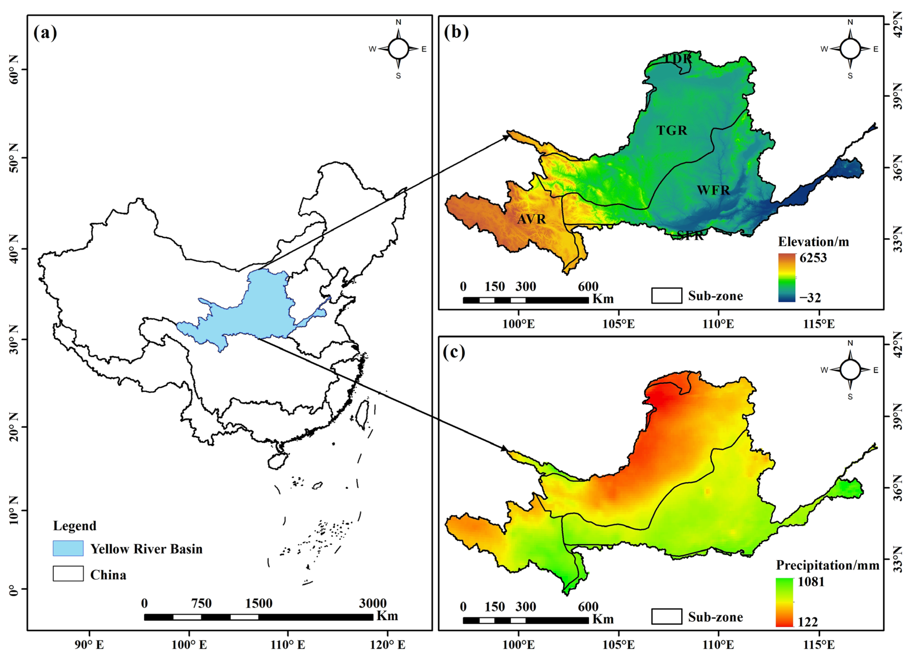
2.1. Study Area Description

The Yellow River originates in the Bayan Har Mountains in the western part of China and has a total length of 5464 km, making it the second longest river in China. It flows through nine provinces before finally emptying into the Bohai Sea. The YRB lies between latitudes 32° to 42° north and longitudes 96° to 119° east, spanning the eastern, central, and western regions of China, covering a total area of 795,000 km², accounting for 8.3% of China’s terrestrial area (Figure 1). Most parts of the basin are classified as arid or semi-arid regions, with annual precipitation of less than 500 mm. Rainfall is scarce and unevenly distributed, leading to severe water scarcity issues and frequent droughts [48]. The upstream region of the river source has an average elevation of over 4000 m, with low temperatures and sparse precipitation. The middle reaches flow through the Loess Plateau, where soil erosion and water loss are significant issues. The downstream area, with an elevation below 100 m, is primarily composed of the Yellow River alluvial plain [49]. Based on the vegetation types, the YRB can be categorized into the Alpine Vegetation Region (AVR), Temperate Desert Region (TDR), Temperate Grassland Region (TGR), Warm Deciduous Broad-Leaved Forest Region (WFR), and Subtropical Evergreen Broad-Leaved Forest Region (SFR) [50]. The basin has a limited number of rain-fed vegetation, with plants primarily relying on soil water, groundwater, and artificial irrigation for moisture. Considering these factors, studying the response of vegetation to drought is crucial for understanding the ecological adaptation mechanisms, promoting regional water resource management, and encouraging ecological conservation practices in the YRB.

2.2. Dataset

The remote-sensing dataset used includes the Normalized Difference Vegetation Index (NDVI), potential evapotranspiration (ET₀), and actual evapotranspiration (ET_a). The NDVI data were obtained from the AVHRR GIMMS NDVI monthly remote-sensing dataset (8 km × 8 km) provided by the National Earth System Science Data Center. After preprocessing using ArcGIS software, the NDVI data were able to reflect the vegetation growth condition and density in the YRB (1982–2022) [37]. The data were preprocessed and quality controlled to ensure data integrity and logical consistency. The ET₀ data were derived from the monthly potential evapotranspiration dataset (1982–2022) released by the National Tibetan Plateau Data Center (1 km × 1 km). The data were extracted and converted to GeoTIFF format prior to being clipped using ArcGIS software. The dataset was obtained based on the Hargreaves potential evapotranspiration formula using the monthly mean temperature, minimum temperature, and maximum temperature datasets (1 km × 1 km) [51]. The ET_a data were sourced from the comprehensive actual evapotranspiration dataset provided by Harvard University (1 km × 1 km). The monthly GeoTIFF files were first merged together to ensure global coverage, and they then underwent the same processing as the ET₀ data to ensure consistency in the study area and numerical units [52]. The SPEI data were obtained from the Centre for Environmental Data Analysis and were available at a spatial resolution of 5 km for the period from 1982 to 2022 [53]. This dataset provided important and valuable information for drought investigations at the regional and global scales. Meteorological data (including precipitation) related to vegetation’s driving factors were sourced from the Famine Early Warning Systems Network Land Data Assimilation System (FLDAS) dataset, which included various climate-related variables and had global coverage [54]. To ensure consistency in terms of resolution, the preprocessed datasets were resampled to 8 km using the bilinear interpolation method, with the study period covering 1982–2022.

3. Methodology

3.1. Construction of Standardized Drought Index

The drought index constructed based on standardized methods possesses characteristics such as spatial comparability, inclusion of probability information, simplicity of calculation, and ease of interpretation [32,42]. The SPEI was selected as the meteorological drought index. It is calculated by obtaining the cumulative probability values of the difference sequence between precipitation and potential evapotranspiration, followed by a normalization process using the normal distribution [14,30]. Referring to the calculation procedure for the SPEI, we developed the standardized vegetation water-deficit index (SVWI). Firstly, based on the Surface Energy Balance System model, calculations and derivations of the latent heat flux and evapotranspiration were performed using Python, resulting in the vegetation water consumption (VWC). Secondly, the crop coefficient method recommended by the Food and Agriculture Organization of the United Nations (FAO-56) was employed to calculate the vegetation water requirements (VWR). By applying the principle of water balance, the difference between the VWC and the VWR was obtained as the vegetation water deficit (VWD). Probability distribution functions were then used to fit the VWD. Subsequently, the accumulated frequency distribution of the VWD was transformed into a standard normal distribution to derive the SVWI.

$$VWC=[1-exp(-NDVI/NDV{I}_{max})]\times E{T}_a$$

(1)

$$VWR=K_c\times E{T}_0$$

(2)

$$VWD=VWC-VWR$$

(3)

$$F_{yi}={\displaystyle {\int }_{-\infty }^x{f}_{yi}(t)dt}$$

(4)

$$SVWI={\Phi }^{-1}(F_{yi})$$

(5)

where NDVI_max is the maximum NDVI under full vegetation cover; ET_a is the actual evapotranspiration; K_c is the crop coefficient at different growth stages; ET₀ is the potential evapotranspiration; VWC, VWR and VWD are the vegetation water consumption, vegetation water requirements and vegetation water deficit, respectively; F_yi is the cumulative probability; and SVWI is the standardized vegetation water-deficit index.

3.2. Bayesian Estimator of Abrupt Seasonal and Trend Change Algorithm (BEAST)

Based on the nonlinear and non-stationary characteristics of the vegetation and drought time series, the Bayesian estimator algorithm BEAST is used to comprehensively evaluate the dynamic changes of vegetation and drought. The BEAST algorithm decomposes the time series into the seasonal component, trend component and residual component to detect the break points in the seasonal and trend components [23,24]. Suppose an additive decomposition model can be used to iterate a piecewise linear model that matches the seasonal and trend patterns:

$$Y_t=S_t+T_t+R_t t=1,\dots ,n$$

(6)

where Y_t is the observation data at time t; S_t is the periodic components; T_t is the long-term trend component; R_t is the remaining components; and t is the moment of observation.

3.3. Spatial Trend Identification Method

The spatial trend detection method, a non-parametric statistical test, is capable of identifying the spatial trend characteristics within time series. It is based on the assumption that the time series data are random and independent. Traditional time series trend tests determine upward or downward trends based on the obtained statistical values. However, they fail to capture continuous trend characteristics across spatial scales. The improved spatial trend detection methods visually represent the spatial distribution of series trends and are not affected by the autocorrelation of individual series [30,55]. As a statistical test value for spatial trend detection, the Zs, which is greater or less than 0, indicates that vegetation is greening or yellowing, respectively. In this study, we employ the spatial trend detection method to identify the gridded trend characteristics of vegetation in the study area (1982–2022).

3.4. Cross-Wavelet Transform Technology

The wavelet transform is a localized analysis of time and frequency, refining signals or functions at multiple scales through scaling and shifting operations to analyze the multi-level time structure and local features of the signal. Cross-wavelet analysis combines cross-spectral analysis with wavelet transform to analyze the resonance period and phase relationship in the time–frequency domain with certain physical relationships [56]. The wavelet coherence reflects the degree of coherence in the time–frequency space between two time series, while the wavelet coherence spectrum is used to identify regions of common variation in the time–frequency space of the two-time series [57]. In terms of wavelet coherence, the Average Wavelet Coherence (AWC) and Percent Area of Significant Coherence (PASC) are used to quantitatively evaluate the explanatory power of predictor variables on response variables. Additionally, the theory of Partial Wavelet Coherency (PWC) evolved from the theory of coherence analysis. If the coherence coefficient between input signals is too high, using the coherence analysis method to identify noise sources may result in significant errors. The PWC method takes this issue into account by eliminating the influence between input signals before conducting the coherence analysis. Therefore, when the influence between input signals is significant in relation to noise source identification, the method of identifying noise sources using the partial coherence function can yield more accurate results [58]. The Multiple Wavelet Coherence (MWC) is an analytical method for testing the coherence between multiple signals, which can reveal the frequency domain coupling between signals in complex systems. The calculation of the MWC is similar to that of the PWC, as it requires incorporating information from multiple signals into the wavelet transform and coherence calculation. The cross-wavelet spectrum can be represented as:

$$W_n^{XY}(s)=W_n^X(s)W_n^{Y*}(s)$$

(7)

where $W_n^{Y*}(s)$ is the complex conjugate of $W_n^Y(s)$, s is the time series, and n is the length of s. The larger the value of $|W_n^{XY}(s)|$, the higher the cross-correlation coefficient.

4. Results

4.1. Changes in Vegetation Dynamics

Figure 2 illustrates the characteristics of the monthly SVWI variations in the YRB from 1982 to 2022. The regions with a more pronounced decreasing trend in the SVWI were the AVR and SFR, with linear trend rates of −0.043/10a. The average SVWI values in these regions were −0.003 and −0.005, respectively. The minimum SVWI values in these two regions were observed in March 2022 (−2.12) and December 2022 (−1.90). Across the entire basin, the linear trend rate of the SVWI was −0.017/10a, with the lowest SVWI value (−1.81) occurring in February 2020. Throughout the study period, all the areas of the YRB exhibited a declining trend in the SVWI, although the extent of the decline varied.

In addition to the monthly SVWI, the variation characteristics of the SVWI at different decadal scales are shown in Figure 3. From the 1980s to the 2010s, the mean SVWI values were 0.12, 0.13, −0.18, and −0.03, respectively. Specifically, the SVWI exhibited a gradual decreasing trend in the 1990s and the 2010s, while it showed a gradual increasing trend in the 1980s and the 2000s. In the 1980s, the lower SVWI values were mainly concentrated in the TGR, while the higher values were primarily found in the AVR. Furthermore, the mean SVWI value in the AVR decreased from 0.98 (in the 1980s) to −0.94 (in the 2010s), resulting in a difference of 1.92 between them. From 1982 to 2022, the SVWI in the TGR showed a gradual upward trend. Therefore, the spatial distribution of the SVWI differed across various decades.

Based on the BEAST algorithm, the seasonal component, trend component, and residual of the SVWI in the YRB from 1982 to 2022 are illustrated in Figure 4. Notably, the gray envelope around the change points represents the 95% confidence interval for the occurrence probability. The seasonal components exhibited periodic changes due to phenological variations in vegetation growth. Specifically, there was a 99.52% probability that a seasonal change point occurred in January 2003, with a confidence interval spanning from December 2002 to April 2003. The mean SVWI values before and after this change point were 0.25 and −0.27, respectively. For the trend change points, which typically indicated abrupt greening or browning of vegetation over long study periods, there was a 72.15% probability that a trend change point occurred in June 2002, with a confidence interval from February 2002 to August 2003. The mean SVWI value declined from 0.26 before the change point to −0.28 after it. The trend component of the SVWI showed distinct fluctuation patterns before and after this change point, and this component is of an increase to decrease type.

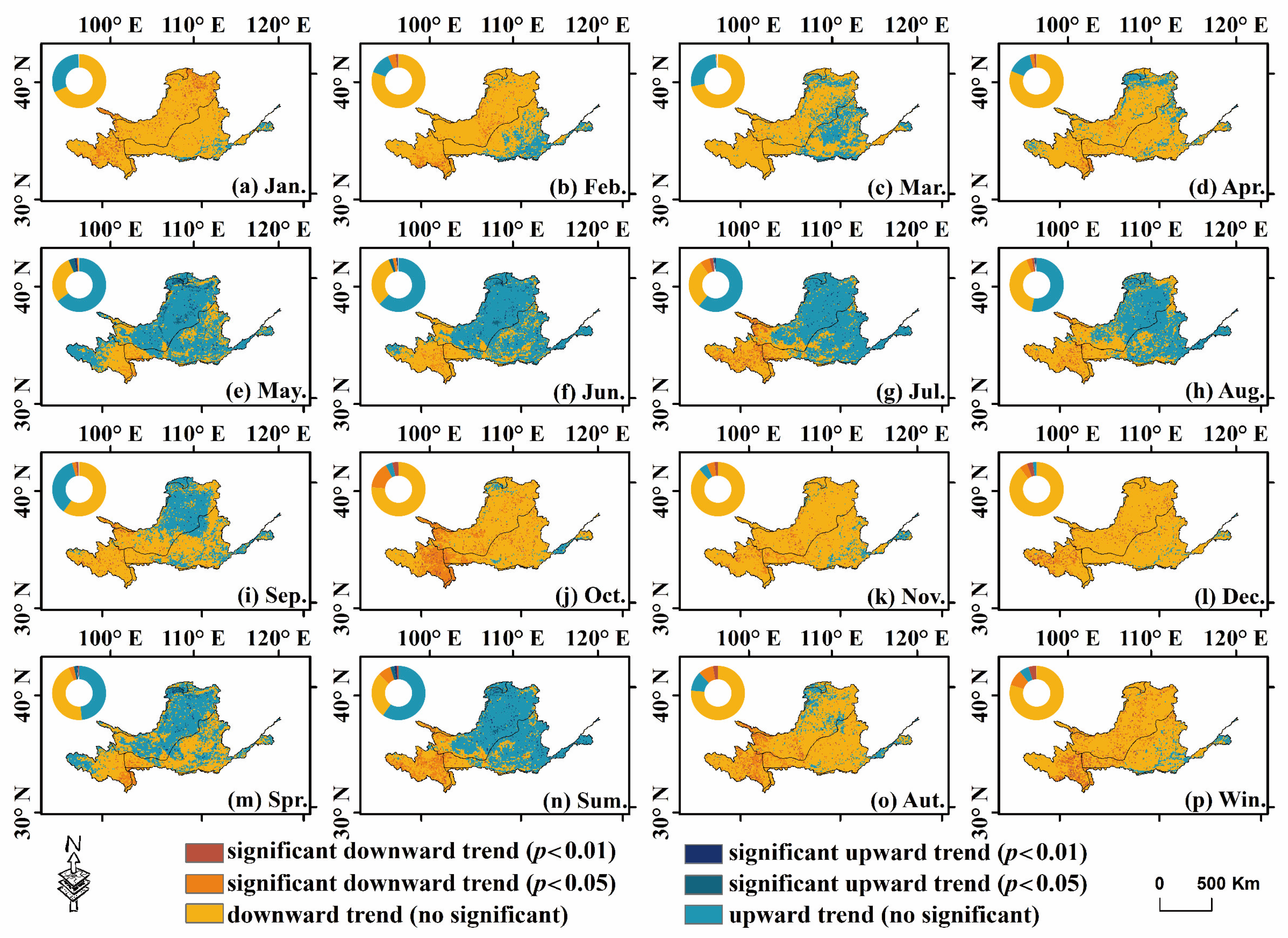
4.2. Spatial Trend Variations of Vegetation

Based on the spatial trend detection method, Figure 5 illustrates the characteristics of the SVWI variation in the YRB from 1982 to 2022. From January to April, the SVWI demonstrated a decreasing trend, with the mean values of the trend statistic Zs being −1.40, −1.01, −0.39, and −0.73 (Figure 6). Conversely, from May to July, the SVWI showed an increasing trend, with high values primarily occurring in the midstream and downstream. The maximum Zs mean value (0.44) occurred in May, with the percentage of area exhibiting an increasing SVWI reaching 69.63%. Subsequently, from August to December, the SVWI exhibited a decreasing trend, with the Zs value reaching its minimum (−1.45) in October. During these months, the percentage of area showing a decreasing SVWI was 97.81% in December and 45.68% in August. It is noteworthy that the Zs values for all the zones in October were less than −1.40, with the Zs value being −1.92 in the AVR. From spring to winter, the mean Zs values of the SVWI in the YRB were −0.04, 0.20, −1.07, and −1.46, respectively. Evidently, the most pronounced decrease in the SVWI occurred in winter, with a percentage area of 94.26%.

4.3. The Spatial Distribution and Recurrence Period of Drought

Based on the SPEI, the most severe drought in the YRB occurred in 1997, with an SPEI value of −1.09. The spatial variation characteristics of the monthly and seasonal drought in that year are shown in Figure 7. From January to April, the drought conditions were not very pronounced, with only a few areas experiencing dry spells. In May, drought began to appear in the WFR, with an SPEI value of −1.01 and a drought area percentage of 32.84%. The spatial distribution of the drought from June to September varied, with the SPEI values ranging from −0.05 to −1.17 and the drought area percentage reaching 68.18% in June. The most severe drought occurred in October, with the SPEI reaching a minimum of −1.44. From November to December, the drought gradually eased, with the drought area percentage being less than 1%. At the seasonal scale, autumn experienced the most severe drought, with a drought area percentage of 74.64%. More importantly, the areas most severely affected by drought were primarily concentrated in the WFR of the YRB.

Copula functions were used to identify the joint return periods of the drought duration and severity in the YRB, and the results are illustrated in Figure 8. In the AVR, TGR, and YRB regions, the optimal copula function for the drought duration and severity was the Frank copula. The number of drought events during the study period was 30, 49, and 45, respectively. In the YRB, a drought event from September 1998 to February 1999 lasted six months, with a severity of 6.48 and a return period of 8.54 years. Additionally, the drought events from May 1997 to October 1997 and from November 2008 to April 2009 each lasted six months, with return periods of between 5 and 10 years. In the AVR, the longest drought duration and highest severity were 7 months and 7.48, respectively. In the TGR, one drought event exceeded a 10-year return period. Generally, greater drought severity corresponds to longer drought duration. In the TDR, WFR, and SFR, the optimal copula functions were the Gaussian copula, Clayton copula, and Gumbel copula, respectively. The average drought severities in these regions were 2.07, 2.17, and 2.45. In the TDR, one drought event (October 2008 to April 2009) had a return period of 10.89 years. Clearly, in the YRB, higher drought severity is associated with longer drought duration.

4.4. The Impacts of Drought Events on Vegetation Growth

Due to the self-regulating capacity of vegetation, meteorological drought does not necessarily lead to vegetation water stress. Therefore, we separately compiled meteorological drought events that did and did not cause vegetation water stress, and we calculated the duration, severity, and severity peaks of these drought events (Figure 9). For the drought duration, the mean duration of the drought events that caused vegetation water stress (Type 1) was 2.63 months, while the mean duration of the drought events that did not cause vegetation water stress (Type 2) was 1.36 months. In terms of the Type 1 drought events, the longest duration (10 months) occurred from July 1986 to April 1987. Similarly, the mean severities for Types 1 and 2 were 2.27 and 1.14, respectively. Regarding the severity peaks, Type 1 exhibited a 25.22% higher severity peak compared to Type 2. In summary, Type 1 exhibited longer durations, greater severity, and higher severity peaks, indicating that severe drought events were likely to have adverse effects on vegetation.

Based on the drought duration, we classified the drought events into short-term (1–2 months), medium-term (3–4 months), and long-term (greater than 4 months) events (Figure 10). Across the various sub-regions of the YRB, the meteorological drought severity (MDS) and vegetation growth status (VGS) exhibited consistent fluctuations, demonstrating a close relationship between vegetation growth and drought. In the AVR, the number of short-term, medium-term, and long-term drought events was 14, 13, and 3, respectively. Moreover, for the short-term, medium-term, and long-term droughts, the MDS exceeded the VGS by 32.21%, 28.97%, and 17.17% on average, with slopes of 0.41, 0.12, and −0.23, respectively. In the other sub-regions, the highest number of drought events (52) occurred in the WFR, with an average MDS and VGS of 2.17 and 1.15, respectively. Conversely, the lowest number of drought events (25) was observed in the SFR. Overall, as the drought duration increased, the sensitivity of vegetation to drought events gradually weakened.

5. Discussion

5.1. Driving Factor Identification

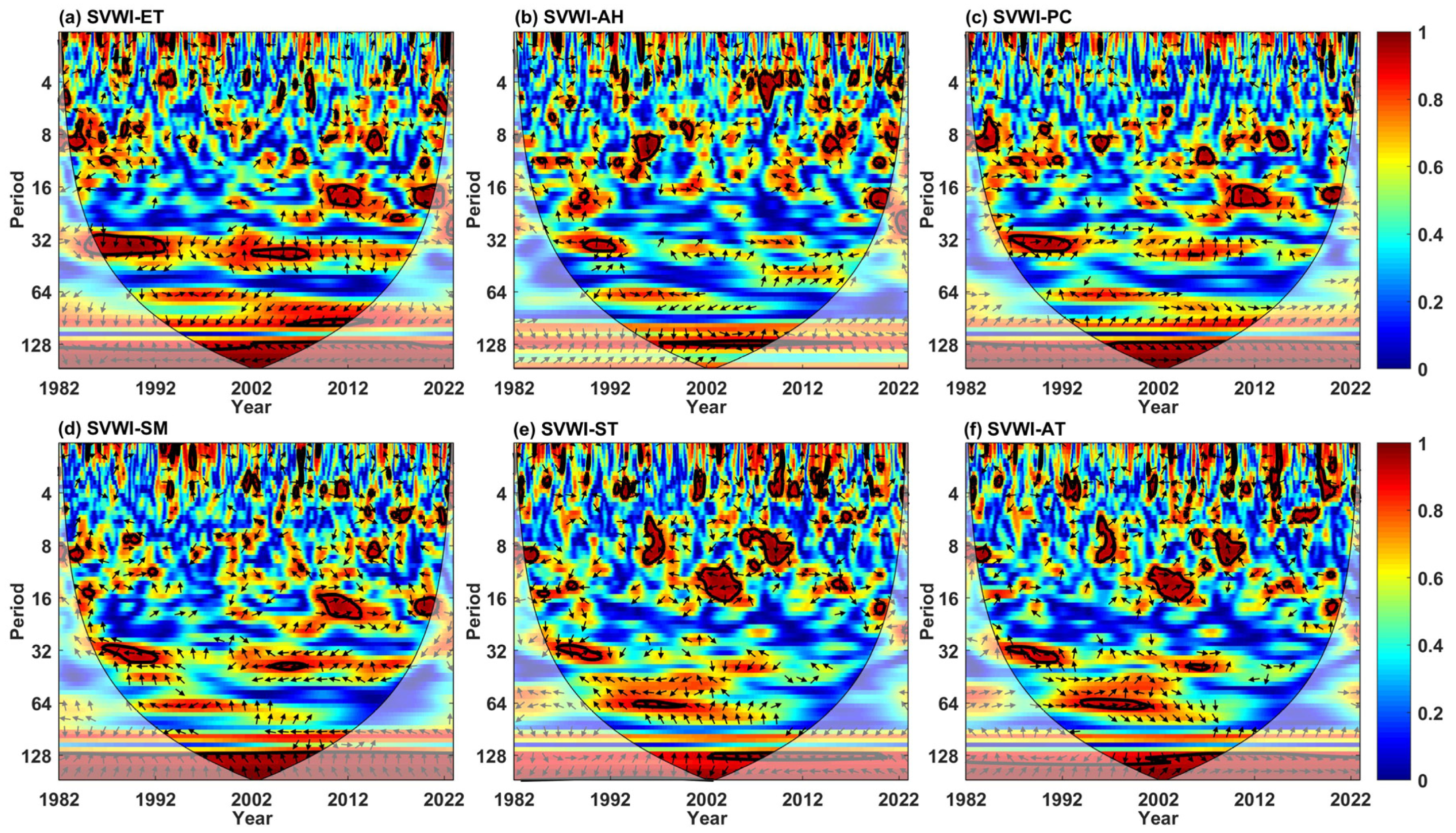
5.1.1. Univariate Influencing Factors

To elucidate the scale effects between different climatic factors and vegetation growth, we selected several representative influencing factors, such as evapotranspiration (ET), air humidity (AH), precipitation (PC), soil moisture (SM), soil temperature (ST), and air temperature (AT). Clearly, these factors are important covariates in the vegetation growth process and are closely associated with vegetation growth. Figure 11 displays the PWC between vegetation and a potential driving factor after eliminating some variable interference. The rightward and leftward arrows indicate the positive and negative phase relationships, and the color bar represents the energy density. Specifically, we divided the time–frequency scale into three subparts: large-scale (>32 months), small-scale (<8 months), and medium-scale (8–32 months) events. Overall, the vegetation and climate factors exhibited complex coherence at the small and medium time–frequency scales, with continuously changing phase angles. At the large time–frequency scale, the phase angle changes were relatively stable. After eliminating the influences of the AH, PC, SM, ST, and AT, the high-energy coherence region between the SVWI and the ET in the time–frequency domain mainly concentrated on large-scale cycles exceeding 32 months, with a predominantly negative phase relationship at different scales. In detail, at the small scale, the SVWI and ET showed significant intermittent resonance periods, with AWC and PASC values of 0.91 and 7.22%, respectively (

Table 1. The AWC and PASC values between the SVWI and meteorological elements (ET, AH, PC, SM, ST, and AT) at the small, medium, and large scales.

PWC	Scale	ET	AH	PC	SM	ST	AT
AWC	Small	0.91	0.91	0.91	0.91	0.91	0.91
	Medium	0.91	0.90	0.90	0.90	0.91	0.91
	Large	0.97	0.92	0.96	0.96	0.95	0.96
	Total	0.96	0.91	0.95	0.95	0.92	0.94
PASC (%)	Small	7.22	5.89	2.75	4.42	6.92	5.41
	Medium	5.82	4.48	6.33	4.21	5.34	5.06
	Large	26.27	3.02	21.98	24.67	6.21	19.40
	Total	13.56	4.35	10.94	12.14	6.47	11.24

). At the medium scale, there were four resonance periods between the SVWI and the ET: 28–32 months (1985–1992), 16–24 months (2009–2013), 8–12 months (2014–2015), and 16–24 months (2018–2020), with AWC and PASC values of 0.91 and 5.82%, respectively. At the large scale, two distinct resonance periods existed between the SVWI and the ET: 128–160 months (1998–2008) and 96–118 months (2006–2014), with AWC and PASC values of 0.97 and 26.27%, respectively. The phase coherence between the SVWI and the AH indicated inconsistent phase relationships in different time–frequency domains, suggesting complex nonlinear interactions between them at different periodic scales. The resonance periods of the SVWI and the PC at the small scale were relatively weak, with significant high-energy coherence regions primarily distributed in interannual and decadal-scale periods. Similarly, the PWC of the SVWI and other climate factors is shown in Figure 11. At the medium scale, the PC has the greatest impact on the SVWI (PASC = 6.33%), while at the small and large scales, the ET has the greatest impact on the SVWI, with PASC values of 7.22% and 26.27%, respectively. In addition, at all the time–frequency scales, the ET and SVWI have the highest AWC (0.96) and PASC (13.56%), making the ET the best explanatory variable for explaining vegetation changes in the YRB.

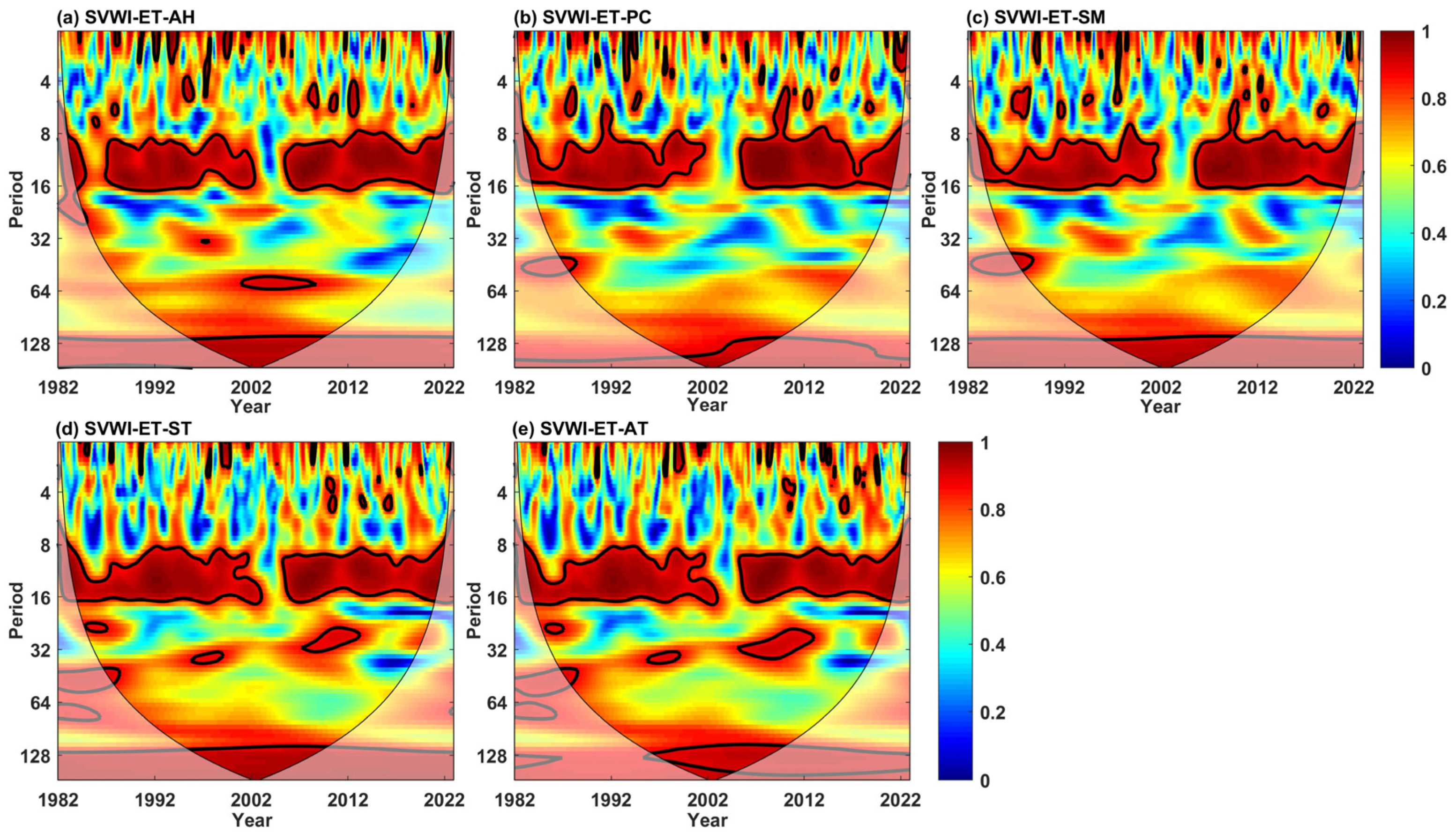
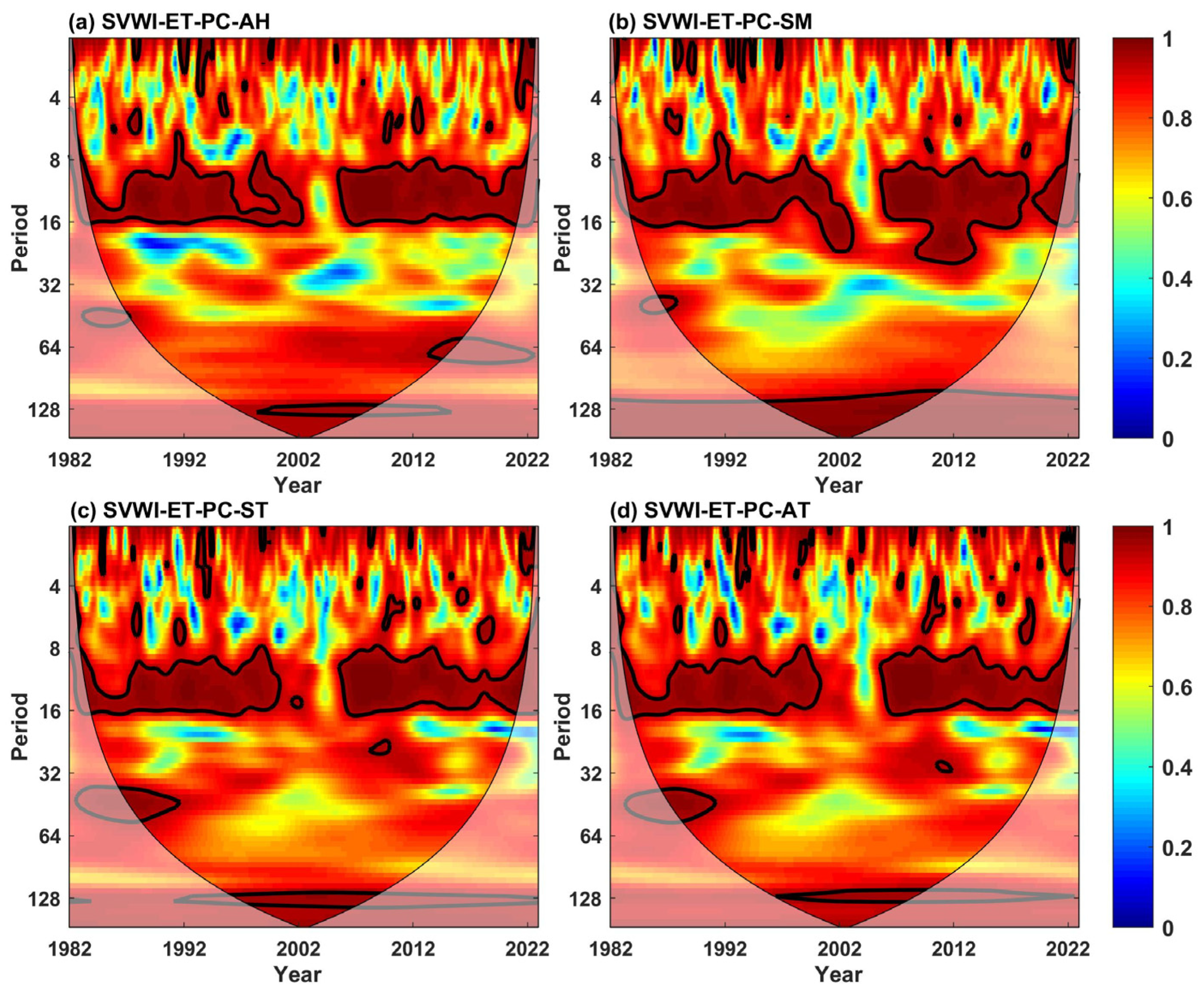
5.1.2. Multivariate Influencing Factors

The independent impact factor makes it difficult to explicate the multiscale features and complex variability of vegetation. The MWC can provide a new solution to reveal the synergistic effects of multiple driving factors on vegetation. Figure 12 shows the MWC of different driving factors on the multiscale feature variability of vegetation. Meanwhile, the coupling effect between climate variables can better elucidate the multiscale feature variations of vegetation in the YRB. The maximum values of two climate factors coupling appeared in the ET–PC combination, with AWC and PASC values of 0.93 and 23.85%, respectively, indicating that the bivariate impact factors ET and PC simultaneously played dominant roles in vegetation change. At the small time–frequency scale, there were multiple small intermittent resonance periods between the ET–PC and the SVWI. At the medium scale, there were mainly two mutual periods between the ET–PC and the SVWI, which were 8–16 months (1983–2001) and 8–16 months (2005–2020). At the large scale, there were clearly two resonance periods between the ET–PC and the SVWI, which were 40–56 months (1987–1988) and 96–160 months (2000–2009). The main controlling factors that affect vegetation varied with different time–frequency scales. For the bivariate factors, the interaction effect of ET–PC was strong in explaining the vegetation changes.

When three climate factors are coupled, the explanation of the driving factors for the multiscale features of vegetation is improved in all the time–frequency domains (Figure 13). As shown in

Table 2. The AWC and PASC values between the SVWI and climate factors (PC, AT, ST, AH, SM, and ET) based on the MWC.

Univariate	AWC	PASC (%)	Bivariate	AWC	PASC (%)	Trivariate	AWC	PASC (%)
ET	0.96	13.56	ET-AH	0.93	22.57	ET-PC-AH	0.96	14.44
AH	0.91	4.35	ET-PC	0.93	23.85	ET-PC-SM	0.97	24.49
PC	0.95	10.94	ET-SM	0.93	22.29	ET-PC-ST	0.96	15.48
SM	0.95	12.14	ET-ST	0.93	18.80	ET-PC-AT	0.96	14.76
ST	0.92	6.47	ET-AT	0.92	19.33
AT	0.94	11.24

, ET–PC–SM was the optimal three-variable combination for explaining the dynamic vegetation changes (AWC = 0.97, PASC = 24.49%). At the medium time–frequency scale, there were three resonance periods between the ET–PC–SM and the SVWI, which mainly occurred in 8–24 months (1983–2002), 8–28 months (2005–2018), and 8–16 months (2019–2021). At the large scale, there were two mutual periods between the ET–PC–SM and the SVWI, which appeared in 36–48 months (1986–1988) and 96–160 months (1995–2010). Obviously, the relationship between the ET–PC–SM and the SVWI had become closer since 2000, which also meant that the effect of the climate variables ET, PC, and SM had been strengthened since the 21st century. Moreover, for all the three-variable climate factors, their relationship with vegetation was relatively close at the medium scale. At all the scales, the ET–PC–SM and SVWI had the highest PASC, so they could be used as the best variables to explain the vegetation changes.

5.2. Advantages and Limitations

With the continuous maturation of remote-sensing technology, more and more scholars are using remote-sensing data to construct vegetation indices [8,22,59]. The spectral characteristics of canopy reflection can reflect the strength of vegetation activity; thus, most vegetation indices derive different vegetation information by processing the visible and near-infrared bands in satellite data [21,23]. However, vegetation index variation is also influenced by other factors, such as floods, wildfires, pests, hail, and human activities [60]. Therefore, relying solely on vegetation indices without considering the actual water deficit conditions makes it difficult to conduct timely and effective drought warnings and mitigation efforts. In contrast to traditional remote-sensing vegetation indices, the vegetation index constructed in this study can reflect the actual dynamic balance of the vegetation water supply and demand during drought processes, which is helpful for practical application by policymakers [32]. As meteorological and hydrological elements and the land surface vegetation status change over time, the balance between the vegetation water demand and consumption undergoes continuous changes [9,19,22]. By considering land surface hydrological elements and vegetation factors, this study, with the vegetation water shortage as the starting point, employed a standardized transformation method similar to the SPEI for constructing the SVWI. Specifically, −0.5, −1, −1.5, and −2 are considered as the SPEI thresholds for different types of drought [44]. Due to its flexible time scale, simple form, and strong spatiotemporal comparability, the SPEI has great potential for application in monitoring the distribution of drought. Additionally, one of the limitations of the SPEI is its sensitivity to calculating potential evapotranspiration, which may overestimate the contribution of temperature anomalies to drought. From the perspective of the energy and water balance dynamics in the vegetation growth process, this can provide a better mechanistic explanation of vegetation drought processes [42]. Furthermore, the standardized method can reflect the multi-timescale characteristics of vegetation and drought changes, facilitating their combination with other standardized drought indices for the study of the relationships between different types of droughts [14,30,61]. Therefore, the constructed SVWI is a more ideal vegetation drought assessment index.

In recent years, the increase in temperature (0.316 °C/10a) and decrease in precipitation (−5.123 mm/10a) may be among the main reasons for the changes in vegetation greenness [62,63]. Due to the least precipitation (350.92 mm) and sustained high temperatures occurring in 1997, a severe drought occurred in that year, which is consistent with our results [44]. In 1997, the YRB experienced a dry flow for 226 days [64]. In addition, within the five sub-regions of the YRB, the areas of the AVR and TGR accounted for 58.7% of the total basin area. Therefore, the fitted copula function within these two sub-regions contributed to the optimal fitted function for the entire basin (Figure 8).

Table 3. The formulas and parameters of the copula in this study.

Copula Families	Mathematical Descriptions	Parameter Settings
Gaussian copula	${\displaystyle {\int }_{-\infty }^{{\varphi }^{-1}(u)}{\displaystyle {\int }_{-\infty }^{{\varphi }^{-1}(v)}\frac{1}{2\pi \sqrt{1-{\theta }^2}}}}\exp ({\displaystyle \frac{2\theta xy-x^2-y^2}{2(1-{\theta }^2)}})dxdy$	$\theta \in [-1,1]$
t copula	${\displaystyle {\int }_{-\infty }^{t_{{\theta }_2}^{-1}(u)}{\displaystyle {\int }_{-\infty }^{t_{{\theta }_2}^{-1}(v)}\frac{\Gamma (({\theta }_2+2)/2)}{\Gamma ({\theta }_2/2)\pi {\theta }_2\sqrt{1-{\theta }_1{ }^2}}}}{(1+{\displaystyle \frac{x^2-2{\theta }_{1}xy+y^2}{{\theta }_2}})}^{({\theta }_2+2)/2}dxdy$	${\theta }_1\in [-1,1]$$\mathrm{and} {\theta }_2\in (0,\infty )$
Clayton copula	$\max {(u^{-\theta }+v^{-\theta }-1,0)}^{-1/\theta }$	$\theta \in [-1,\infty )$\0
Frank copula	$-{\displaystyle \frac{1}{\theta }}\ln [1+{\displaystyle \frac{(\exp (-\theta u)-1)(\exp (-\theta v)-1)}{\exp (-\theta )-1}}]$	$\theta \in R\backslash 0$
Gumbel copula	$\exp \left\{-{[{(-\ln (u))}^{\theta }+{(-\ln (v))}^{\theta }]}^{1/\theta }\right\}$	$\theta \in [1,\infty )$

lists the formulas and parameters of the copula functions in this study. Consistent with the optimal copula functions in these two sub-regions, the optimal copula function for the entire basin was also the Frank copula, which is reasonable. The characteristics of the identified drought events within the YRB indicate that the greater the severity of drought, the longer the corresponding duration. This study explored the impact of drought on vegetation and revealed the response mechanism of vegetation to environmental changes, which is of practical significance for the dynamic monitoring of droughts, environmental governance, and vegetation protection [5,53]. Before the onset of drought, drought prevention and resistance measures should be formulated in advance to reduce the adverse effects of drought on vegetation growth. For instance, in drought-prone areas, water-saving irrigation technology, dryland agriculture, and drought-resistant management can be enhanced. In summary, clarifying the impact of drought on vegetation growth can provide reference information for policymakers and practitioners.

When other variables are related to the independent variable, the presence of the other variables may affect the accurate representation of the relationship between the independent and dependent variables [57]. The partial wave coherence between input factors facilitates a better understanding of the true correlation between signals [56]. Based on cross-wavelet technology, the factors most closely related to vegetation are the ET and PC in the YRB (Figure 12). The ET connects the process of water and surface energy transmission in vegetation, serving as a central link in the climate system [51,52]. When drought occurs, an increase in the ET may lead to vegetation water shortage, thereby affecting the normal physiological activities of vegetation. As an important source of vegetation water input, the PC affects photosynthesis in vegetation, providing necessary water and nutrients for plant growth [19,36,65]. Wen et al. also found that the ET and PC are closely related to vegetation, and this is also consistent with the reality [66].

Although the vegetation index proposed in this study considers the climatic and hydrological factors of vegetation growth, reflecting the dynamic energy and water balance, limitations still exist due to the data constraints [42]. Because of the difficulty in searching for crop type data and field experimental data, monthly scale data were used to calculate the ecological water demand in this study. Future research could attempt to use daily scale data, establish a three-dimensional database of the soil–root depth–crop type, and combine the corresponding vegetation growth period to further improve the accuracy of the vegetation coefficients, soil moisture restriction coefficients, and ecological water demand calculations [14,32].

5.3. Future Prospects

In the future, several aspects are worth further investigation. Accurately calculating the VWD is crucial for constructing vegetation water deficit indices; however, there is a significant spatiotemporal heterogeneity in the VWD of different vegetation types [21]. As the minimum water requirement for vegetation to fulfill its ecological functions, the VWD is a key indicator in land ecological drought studies [2]. Future research could utilize higher-resolution land use data and combine the experimental results of vegetation evapotranspiration in different regions to accurately infer the spatiotemporal distribution of the VWD [32,42]. Additionally, vegetation is influenced by factors such as the soil moisture, precipitation, and crop type, which introduce uncertainties in predicting future vegetation conditions [67]. With the improvement in the spatiotemporal resolution of remote-sensing data, the uncertainties in extracting vegetation phenological information can be reduced.

6. Conclusions

This study utilized remote-sensing datasets to investigate the seasonal and abrupt changes in vegetation based on the BEAST algorithm in the YRB from 1982 to 2022, revealing the trend characteristics of vegetation at a spatial scale. Subsequently, the spatial distribution of typical droughts and the copula-based joint return periods of drought variables were studied to identify the response characteristics of vegetation growth to drought. The main conclusions are as follows:

(1)

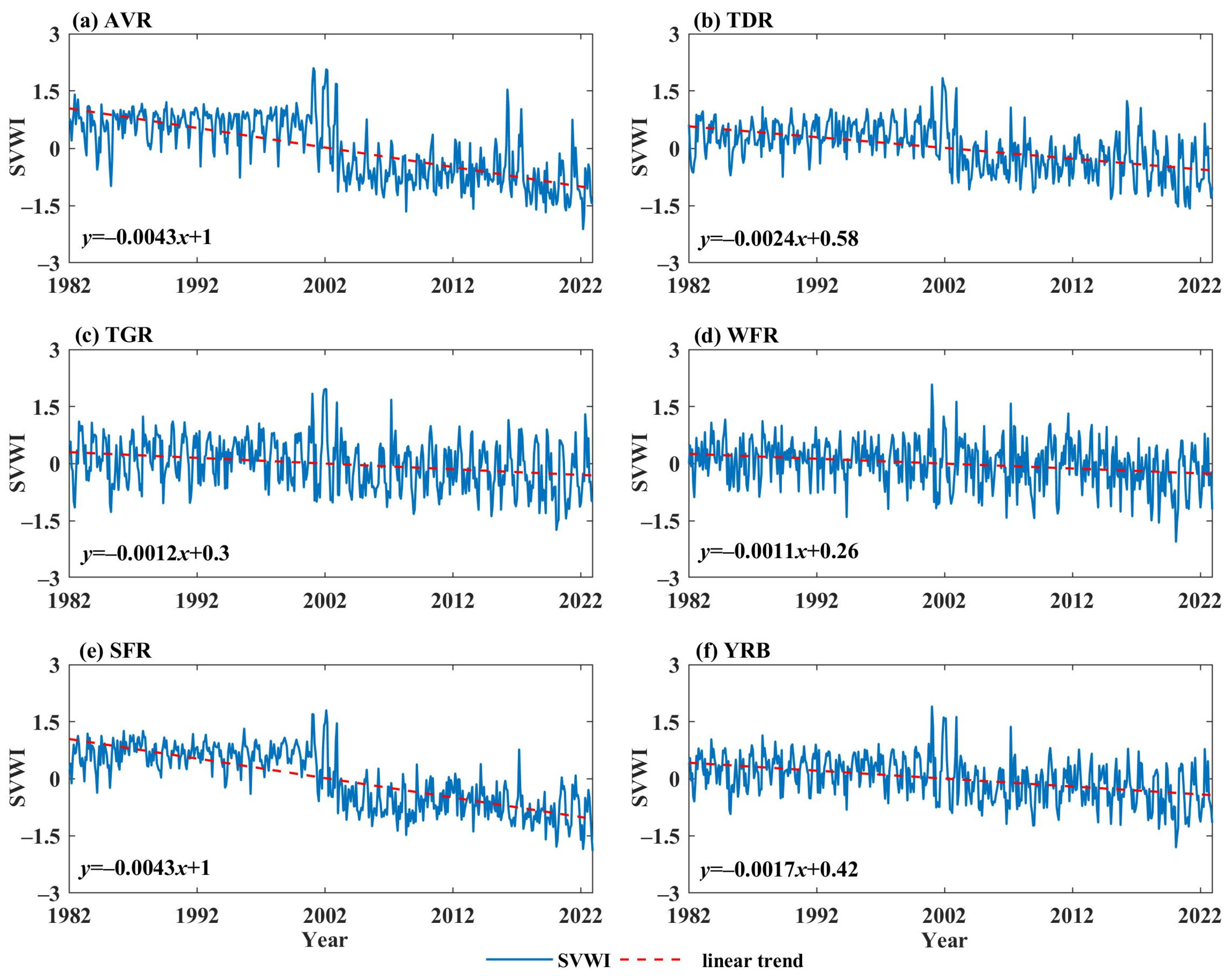
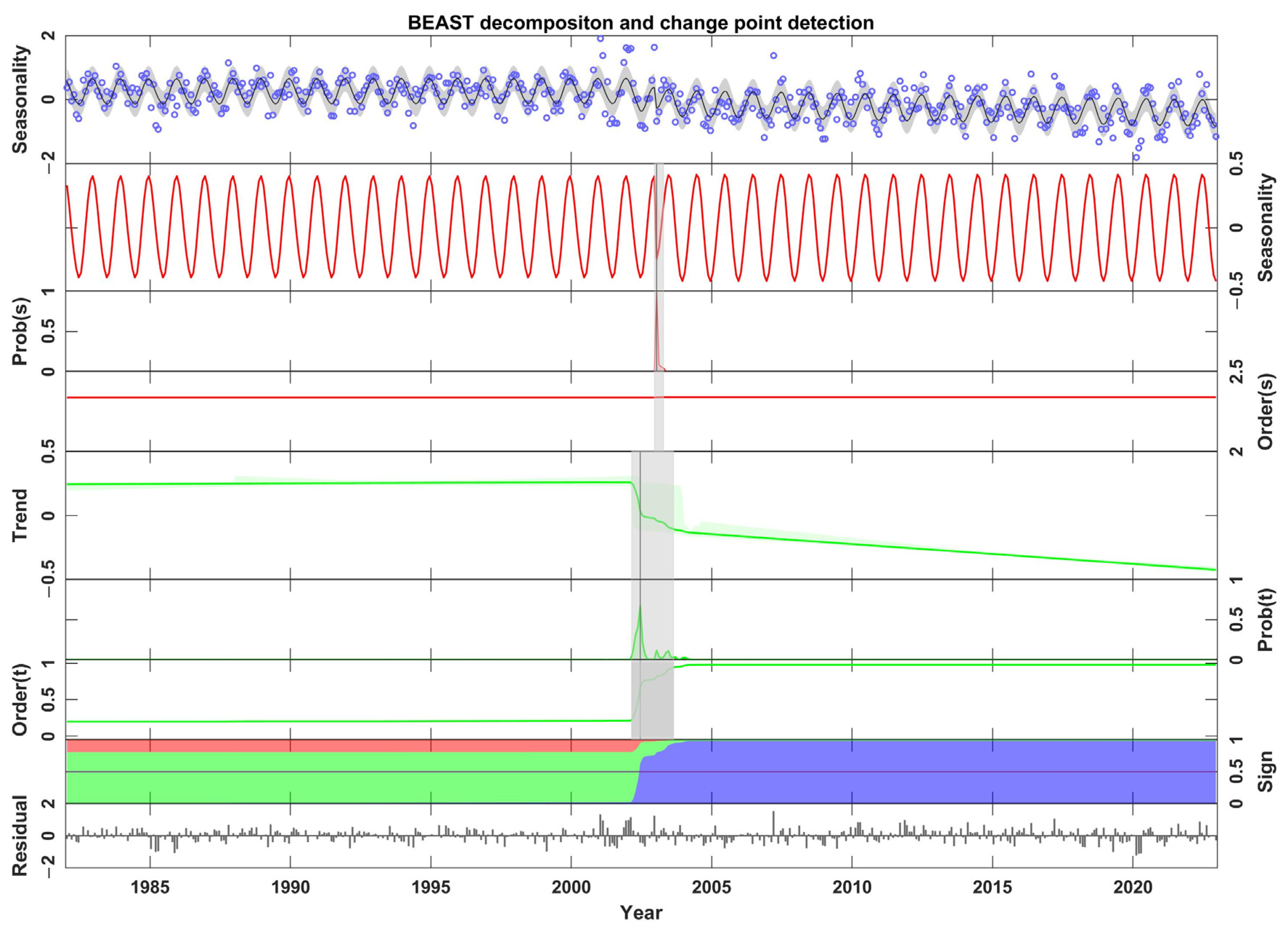
From 1982 to 2022, the SVWI showed a decreasing trend in the YRB, but the magnitude of the decline varied across different sub-regions. At the decadal scale, the SVWI exhibited a gradual decline in the 1990s and 2010s. Based on the BEAST algorithm, the seasonal change point of the SVWI occurred with a probability of 99.52% in January 2003, while the trend change point had a probability of 72.15% in June 2002.

(2)

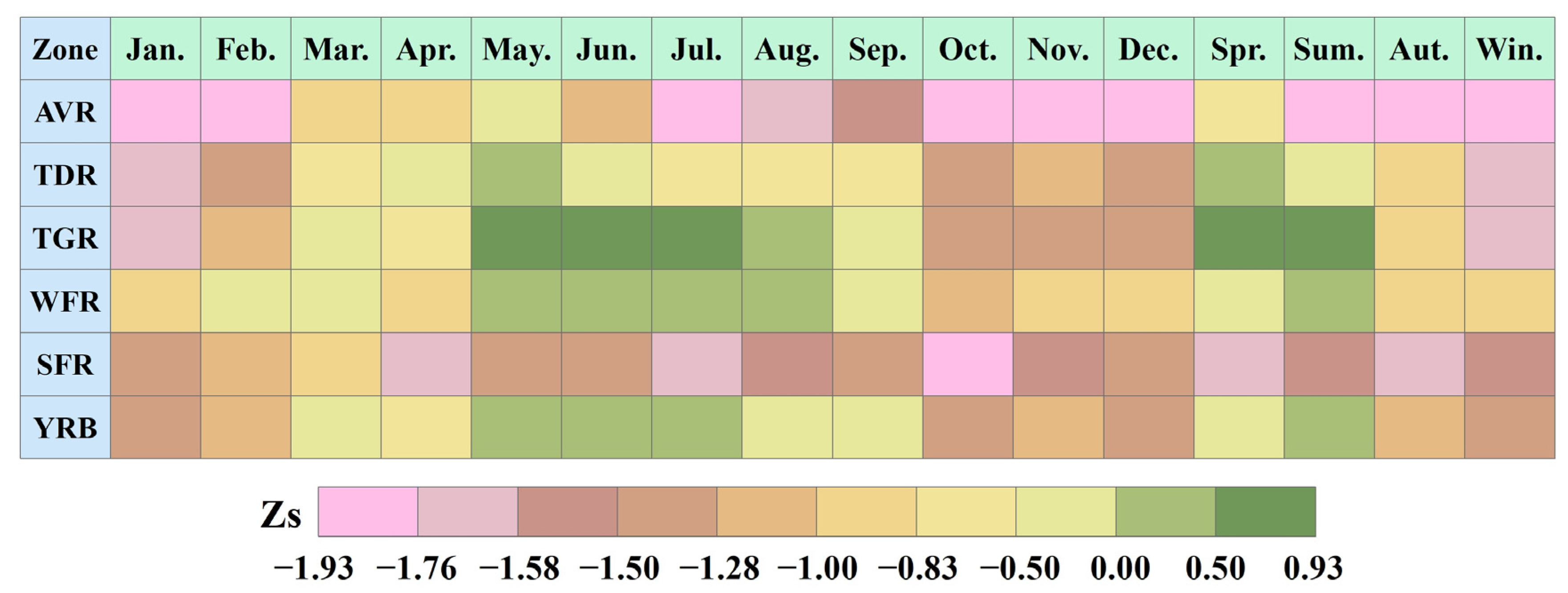
Using the spatial trend identification method, at the grid scale, the SVWI generally increased from May to July and decreased in the other months. Additionally, the minimum value of the trend characteristic Zs, −1.45, occurred in October. Across the different quarters, the range of mean Zs values was −1.46 (winter) to 0.20 (summer), indicating a more pronounced declining trend in winter, with an area percentage reaching 94.26%.

(3)

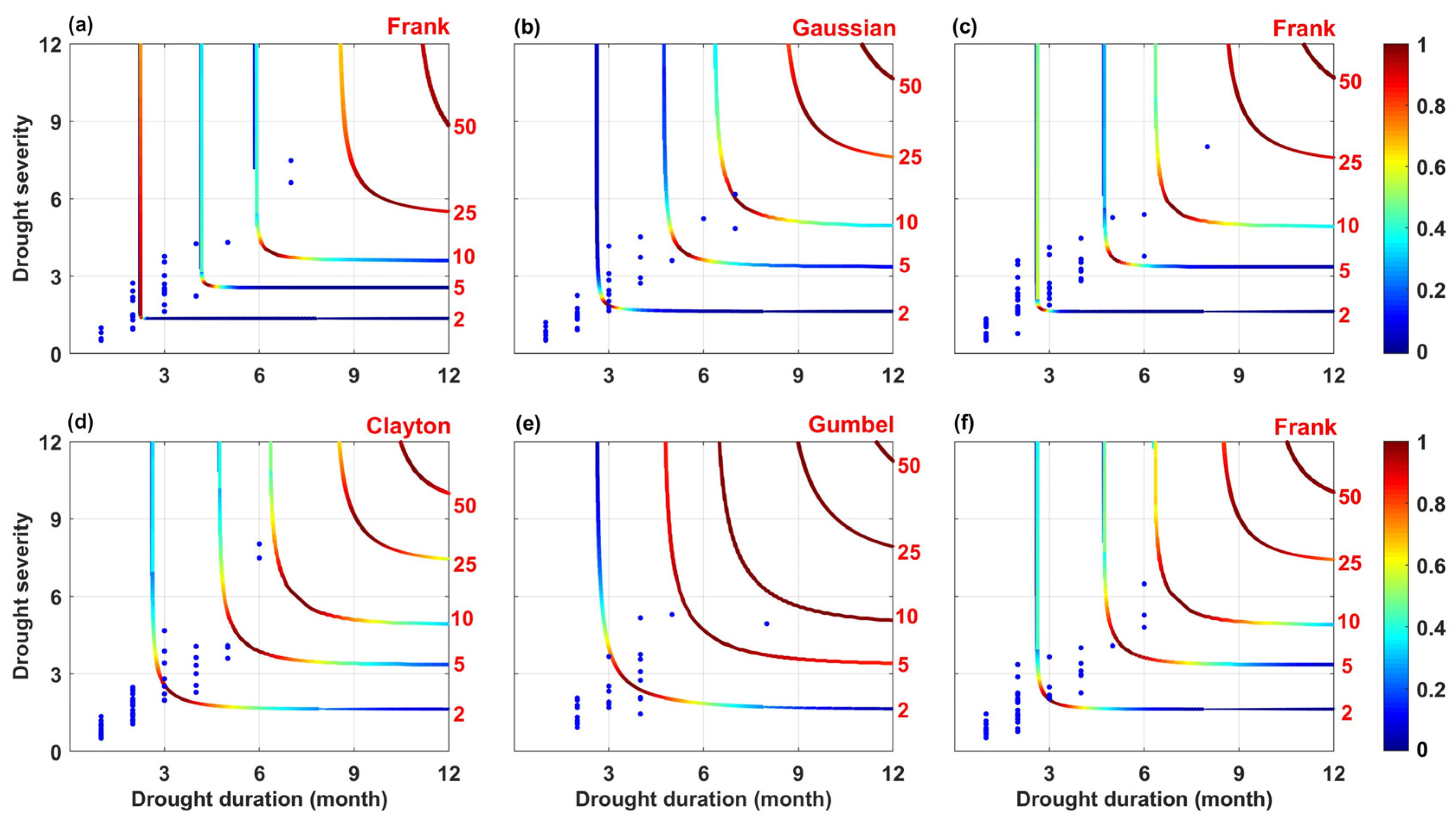
The most severe drought occurred in 1997 within the study period, with an SPEI value of −1.09. In October of that year, the SPEI reached its minimum value of −1.44. Furthermore, the optimal copula function connecting drought variables in the AVR, TGR, and YRB regions was the Frank copula. In the entire basin, the duration of the drought that occurred from September 1998 to February 1999 was 6 months, with a severity of 6.48 and a return period of 8.54 years.

(4)

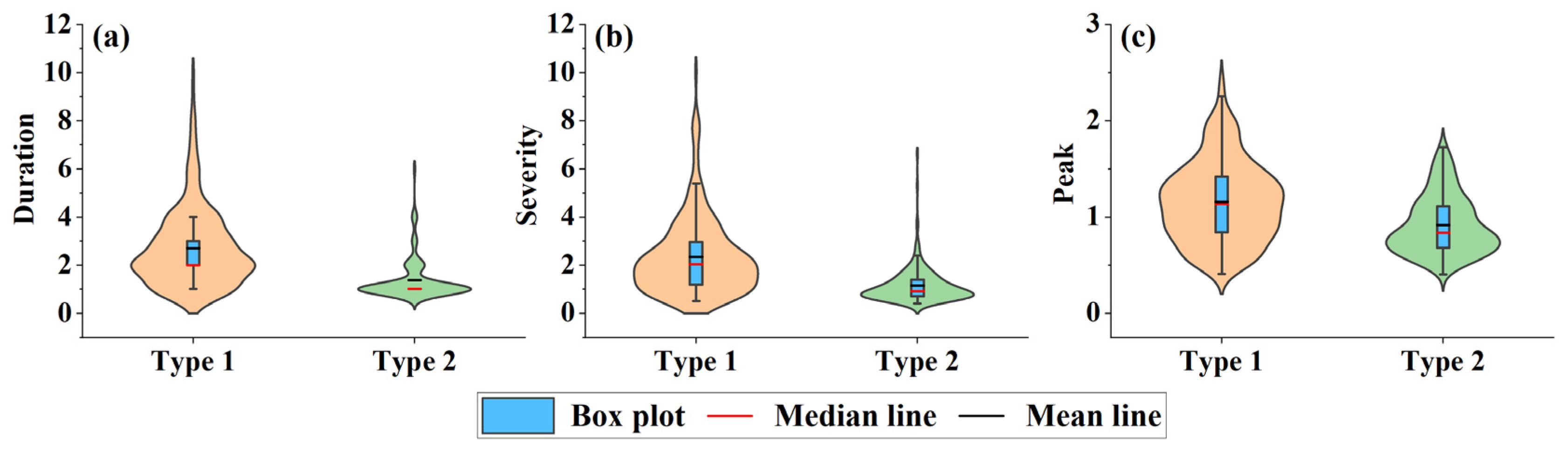
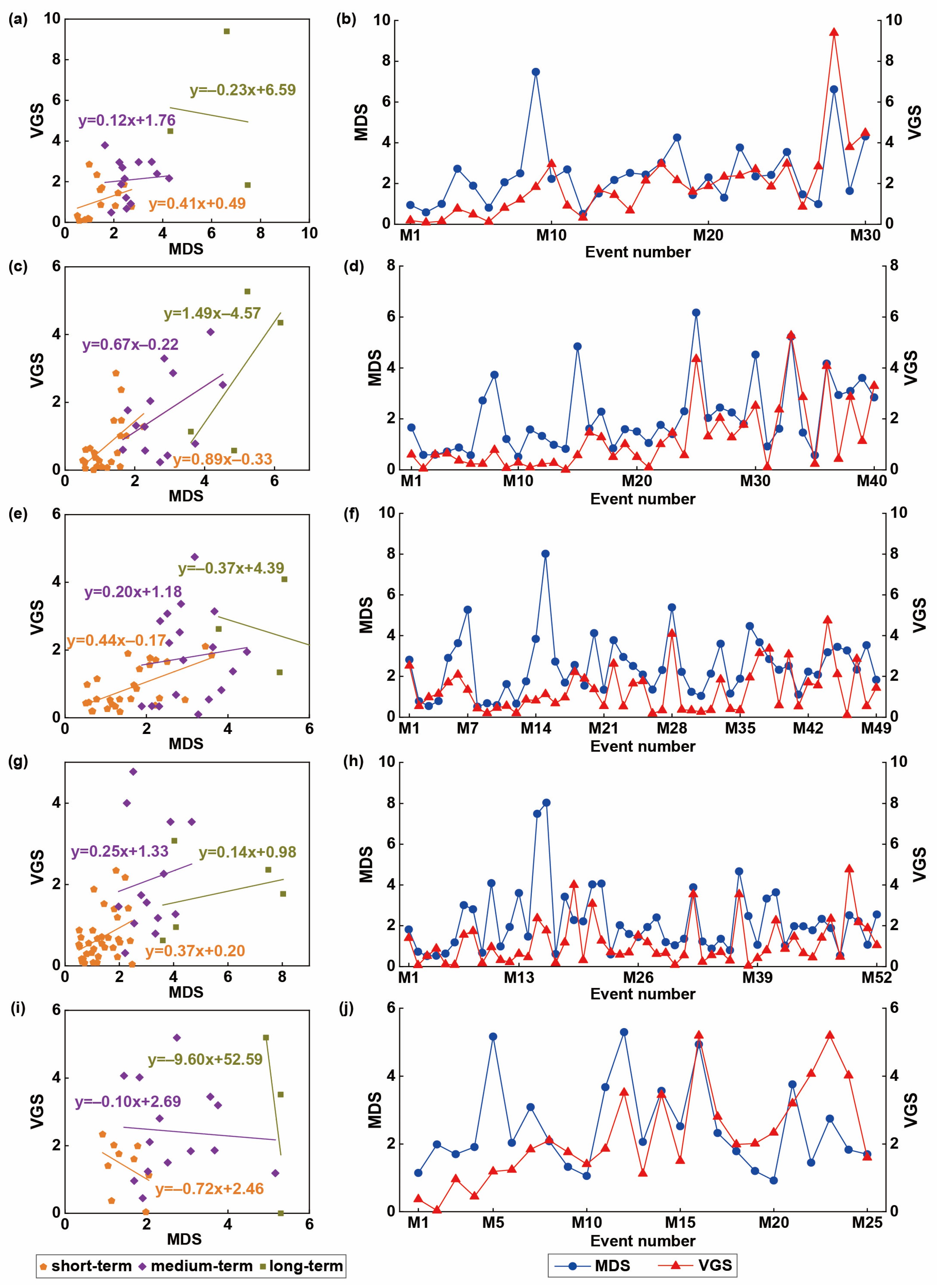
Overall, there was a close relationship between drought and vegetation growth in the YRB. The maximum number of drought events (52 times) occurred in the WFR, while the minimum number of drought events (25 times) occurred in the SFR. Particularly, the MDS of the short-term, medium-term, and long-term drought events in the AVR was 32.21%, 28.97%, and 17.17% higher than the mean of VGS.

(5)

The accuracy of the vegetation water consumption and demand used to calculate the degree of vegetation water shortage may introduce some uncertainty into the results. In the future, we will adopt higher-resolution land-use data to accurately obtain the vegetation water consumption and demand, which will also be our main research focus in the next work.

References

1. Anderson, M.C.; Zolin, C.A.; Sentelhas, P.C.; Hain, C.R.; Semmens, K.; Tugrul Yilmaz, M.; Gao, F.; Otkin, J.A.; Tetrault, R. The Evaporative Stress Index as an indicator of agricultural drought in Brazil: An assessment based on crop yield impacts. Remote Sens. Environ. 2016, 174, 82–99. [Google Scholar] [CrossRef]
2. Bradford, J.B.; Schlaepfer, D.R.; Lauenroth, W.K.; Palmquist, K.A. Robust ecological drought projections for drylands in the 21st century. Glob. Change Biol. 2020, 26, 3906–3919. [Google Scholar] [CrossRef]
3. Su, B.D.; Huang, J.L.; Mondal, S.K.; Zhai, J.Q.; Wang, Y.J.; Wen, S.S.; Gao, M.N.; Lv, Y.R.; Jiang, S.; Li, A.W. Insight from CMIP6 SSP-RCP scenarios for future drought characteristics in China. Atmos. Res. 2021, 250, 105375. [Google Scholar] [CrossRef]
4. Zhao, S.D.; Jiang, Y.; Wen, Y.; Jiao, L.; Li, W.Q.; Xu, H.; Ding, M.H. Frequent locally absent rings indicate increased threats of extreme droughts to semi-arid Pinus tabuliformis forests in North China. Agric. For. Meteorol. 2021, 308–309, 108601. [Google Scholar] [CrossRef]
5. Ding, Y.J.; Zhang, L.F.; He, Y.; Cao, S.P.; Wei, X.; Guo, Y.; Ran, L.; Filonchyk, M. Spatiotemporal evolution of agricultural drought and its attribution under different climate zones and vegetation types in the Yellow River Basin of China. Sci. Total Environ. 2024, 914, 169687. [Google Scholar] [CrossRef]
6. Otkin, J.A.; Anderson, M.C.; Hain, C.; Svoboda, M.; Johnson, D.; Mueller, R.; Tadesse, T.; Wardlow, B.; Brown, J. Assessing the evolution of soil moisture and vegetation conditions during the 2012 United States flash drought. Agric. For. Meteorol. 2016, 218–219, 230–242. [Google Scholar] [CrossRef]
7. Kang, W.P.; Wang, T.; Liu, S.L. The response of vegetation phenology and productivity to drought in semi-arid regions of northern China. Remote Sens. 2018, 10, 727. [Google Scholar] [CrossRef]
8. Khatri-Chhetri, P.; Hendryx, S.M.; Hartfield, K.A.; Crimmins, M.A.; Leeuwen, W.J.D.V.; Kane, V.R. Assessing vegetation response to multi-scalar drought across the mojave, sonoran, chihuahuan deserts and apache highlands in the Southwest United States. Remote Sens. 2021, 13, 1103. [Google Scholar] [CrossRef]
9. Huete, A. Ecology: Vegetation’s responses to climate variability. Nature 2016, 531, 181–182. [Google Scholar] [CrossRef]
10. Pei, F.S.; Wu, C.J.; Liu, X.P.; Li, X.; Yang, K.Q.; Zhou, Y.; Wang, K.; Xu, L.; Xia, G.R. Monitoring the vegetation activity in China using vegetation health indices. Agric. For. Meteorol. 2018, 248, 215–227. [Google Scholar] [CrossRef]
11. Chen, Q.; Timmermans, J.; Wen, W.; van Bodegom, P.M. Ecosystems threatened by intensified drought with divergent vulnerability. Remote Sens. Environ. 2023, 289, 113512. [Google Scholar] [CrossRef]
12. Zhong, S.B.; Sun, Z.H.; Di, L.P. Characteristics of vegetation response to drought in the CONUS based on long-term remote sensing and meteorological data. Ecol. Indic. 2021, 127, 107767. [Google Scholar] [CrossRef]
13. Weng, Z.; Niu, J.; Guan, H.D.; Kang, S.Z. Three-dimensional linkage between meteorological drought and vegetation drought across China. Sci. Total Environ. 2023, 859, 160300. [Google Scholar] [CrossRef]
14. Vicente-Serrano, S.M.; Gouveia, C.; Camarero, J.J.; Beguería, S.; Trigo, R.; López-Moreno, J.; Azorín-Molina, C.; Pasho, E.; Lorenzo-Lacruz, J.; Revuelto, J.; et al. Response of vegetation to drought time-scales across global land biomes. Proc. Natl. Acad. Sci. USA 2012, 110, 52–57. [Google Scholar] [CrossRef]
15. Zhao, X.; Wei, H.; Liang, S.L.; Zhou, T.; He, B.; Tang, B.; Wu, D.H. Responses of natural vegetation to different stages of extreme drought during 2009–2010 in southwestern China. Remote Sens. 2015, 7, 14039–14054. [Google Scholar] [CrossRef]
16. Xu, H.J.; Wang, X.P.; Zhao, C.Y.; Yang, X.M. Diverse responses of vegetation growth to meteorological drought across climate zones and land biomes in northern China from 1981 to 2014. Agric. For. Meteorol. 2018, 262, 1–13. [Google Scholar] [CrossRef]
17. Geldenhuys, C.; van der Merwe, H.; van Rooyen, M.W. Vegetation response to grazing and drought (13 yr) in a conservation area in the Succulent Karoo, South Africa. J. Arid Environ. 2023, 219, 105093. [Google Scholar] [CrossRef]
18. Kogan, F. World droughts in the new millennium from AVHRR-based vegetation health indices. Eos Trans. Am. Geophys. Union. 2011, 83, 557–563. [Google Scholar] [CrossRef]
19. Prăvălie, R.; Sîrodoev, I.; Nita, I.-A.; Patriche, C.; Dumitraşcu, M.; Roşca, B.; Tişcovschi, A.; Bandoc, G.; Săvulescu, I.; Mănoiu, V.; et al. NDVI-based ecological dynamics of forest vegetation and its relationship to climate change in Romania during 1987–2018. Ecol. Indic. 2022, 136, 108629. [Google Scholar] [CrossRef]
20. Ahmad, M.H.; Abubakar, A.; Ishak, M.Y.; Danhassan, S.S.; Zhang, J.H.; Alatalo, J.M. Modeling the influence of daily temperature and precipitation extreme indices on vegetation dynamics in Katsina State using statistical downscaling model (SDM). Ecol. Indic. 2023, 155, 110979. [Google Scholar] [CrossRef]
21. Chi, D.K.; Wang, H.; Li, X.B.; Liu, H.H.; Li, X.H. Estimation of the ecological water requirement for natural vegetation in the Ergune River basin in Northeastern China from 2001 to 2014. Ecol. Indic. 2018, 92, 141–150. [Google Scholar] [CrossRef]
22. Won, J.; Seo, J.; Lee, J.; Lee, O.; Kim, S. Vegetation drought vulnerability mapping using a copula model of vegetation index and meteorological drought index. Remote Sens. 2021, 13, 5103. [Google Scholar] [CrossRef]
23. Cai, Y.T.; Liu, S.T.; Lin, H. Monitoring the vegetation dynamics in the Dongting lake wetland from 2000 to 2019 using the BEAST algorithm based on dense Landsat time series. Appl. Sci. 2020, 10, 4209. [Google Scholar] [CrossRef]
24. White, J.H.R.; Walsh, J.E.; Thoman Jr, R.L. Using Bayesian statistics to detect trends in Alaskan precipitation. Int. J. Climatol. 2021, 41, 2045–2059. [Google Scholar] [CrossRef]
25. Quiring, S.M.; Ganesh, S. Evaluating the utility of the Vegetation Condition Index (VCI) for monitoring meteorological drought in Texas. Agric. For. Meteorol. 2010, 150, 330–339. [Google Scholar] [CrossRef]
26. Sheffield, J.; Wood, E.F.; Roderick, M.L. Little change in global drought over the past 60 years. Nature 2012, 491, 435–438. [Google Scholar] [CrossRef]
27. Zeng, J.; Zhou, T.; Qu, Y.; Bento, V.A.; Qi, J.; Xu, Y.; Li, Y.; Wang, Q. An improved global vegetation health index dataset in detecting vegetation drought. Sci. Data. 2023, 10, 338. [Google Scholar] [CrossRef]
28. Swann, A.L.; Hoffman, F.M.; Koven, C.D.; Randerson, J.T. Plant responses to increasing CO2 reduce estimates of climate impacts on drought severity. Proc. Natl. Acad. Sci. USA 2016, 113, 10019–10024. [Google Scholar] [CrossRef]
29. Zhang, P.; Jeong, J.H.; Yoon, J.H.; Kim, H.; Wang, S.Y.S.; Linderholm, H.W.; Fang, K.; Wu, X.; Chen, D. Abrupt shift to hotter and drier climate over inner East Asia beyond the tipping point. Science 2020, 370, 1095–1099. [Google Scholar] [CrossRef]
30. Wang, F.; Lai, H.X.; Li, Y.B.; Feng, K.; Zhang, Z.Z.; Tian, Q.Q.; Zhu, X.M.; Yang, H.B. Dynamic variation of meteorological drought and its relationships with agricultural drought across China. Agr. Water Manag. 2022, 261, 107301. [Google Scholar] [CrossRef]
31. Wang, F.; Lai, H.X.; Li, Y.B.; Feng, K.; Tian, Q.Q.; Guo, W.X.; Qu, Y.P.; Yang, H.B. Spatio-temporal evolution and teleconnection factor analysis of groundwater drought based on the GRACE mascon model in the Yellow River Basin. J. Hydrol. 2023, 626, 130349. [Google Scholar] [CrossRef]
32. Jiang, T.L.; Su, X.L.; Qu, Y.P.; Singh, V.P.; Zhang, T.; Chu, J.D.; Hu, X.X. Determining the response of ecological drought to meteorological and groundwater droughts in Northwest China using a spatio-temporal matching method. J. Hydrol. 2024, 633, 130753. [Google Scholar] [CrossRef]
33. Mao, J.F.; Shi, X.Y.; Thornton, P.E.; Hoffman, F.M.; Zhu, Z.C.; Myneni, R.B. Global latitudinal-asymmetric vegetation growth trends and their driving mechanisms: 1982–2009. Remote Sens. 2013, 5, 1484–1497. [Google Scholar] [CrossRef]
34. Xu, H.J.; Wang, X.P.; Yang, T.B. Trend shifts in satellite-derived vegetation growth in Central Eurasia, 1982–2013. Remote Sens. Environ. 2017, 579, 1658–1674. [Google Scholar] [CrossRef]
35. Tietjen, B.; Schlaepfer, D.R.; Bradford, J.B.; Lauenroth, W.K.; Hall, S.A.; Duniway, M.C.; Hochstrasser, T.; Jia, G.; Munson, S.M.; Pyke, D.A.; et al. Climate change-induced vegetation shifts lead to more ecological droughts despite projected rainfall increases in many global temperate drylands. Global Change Biol. 2017, 23, 2743–2754. [Google Scholar] [CrossRef]
36. Du, J.; He, Z.B.; Piatek, K.B.; Chen, L.F.; Lin, P.F.; Zhu, X. Interacting effects of temperature and precipitation on climatic sensitivity of spring vegetation green-up in arid mountains of China. Agr. Forest Meteorol. 2019, 269–270, 71–77. [Google Scholar] [CrossRef]
37. Chu, H.S.; Venevsky, S.; Wu, C.; Wang, M.H. NDVI-based vegetation dynamics and its response to climate changes at Amur-Heilongjiang River Basin from 1982 to 2015. Sci. Total Environ. 2019, 650, 2051–2062. [Google Scholar] [CrossRef]
38. Nzabarinda, V.; Bao, A.; Xu, W.; Uwamahoro, S.; Xiaoran, H.; Habiyakare, T.; Sindikubwabo, C.; Habumugisha, J.M.; Itangishaka, A.C. A simple model to predict the spatiotemporally vegetation dynamics in terms of precipitation and temperature. Environ. Dev. 2022, 44, 100769. [Google Scholar] [CrossRef]
39. Nanzad, L.; Zhang, J.; Tuvdendorj, B.; Nabil, M.; Zhang, S.; Bai, Y. NDVI anomaly for drought monitoring and its correlation with climate factors over Mongolia from 2000 to 2016. J. Arid Environ. 2019, 164, 69–77. [Google Scholar] [CrossRef]
40. Zhan, C.; Liang, C.; Zhao, L.; Jiang, S.Z.; Niu, K.J.; Zhang, Y.L. Drought-related cumulative and time-lag effects on vegetation dynamics across the Yellow River Basin, China. Ecol. Indic. 2022, 143, 109409. [Google Scholar] [CrossRef]
41. Niwa, H.; Kamada, M.; Morisada, S.; Ogawa, M. Assessing the impact of storm surge flooding on coastal pine forests using a vegetation index. Landsc. Ecol. Eng. 2023, 19, 151–159. [Google Scholar] [CrossRef]
42. Jiang, T.L.; Su, X.L.; Singh, V.P.; Zhang, G.X. A novel index for ecological drought monitoring based on ecological water deficit. Ecol. Indic. 2021, 129, 107804. [Google Scholar] [CrossRef]
43. Zhao, Y.; Wang, M.Z.; Li, J.; Yang, X.J.; Zhang, N.; Chen, H. Diurnal Variations in Summer Precipitation over the Yellow River Basin. Adv. Meteorol. 2019, 2019, 2482656. [Google Scholar] [CrossRef]
44. Wang, F.; Wang, Z.M.; Yang, H.B.; Zhao, Y. Study of the temporal and spatial patterns of drought in the Yellow River basin based on SPEI. Sci. China Earth Sci. 2018, 61, 1098–1111. [Google Scholar] [CrossRef]
45. Wang, F.; Wang, Z.M.; Yang, H.B.; Di, D.Y.; Liang, Q.H.; Hussain, Z. Comprehensive evaluation of hydrological drought and its relationships with meteorological drought in the Yellow River basin, China. J. Hydrol. 2020, 584, 124751. [Google Scholar] [CrossRef]
46. Li, J.; Xi, M.F.; Pan, Z.W.; Liu, Z.Z.; He, Z.L.; Qin, F. Response of NDVI and SIF to Meteorological Drought in the Yellow River Basin from 2001 to 2020. Water 2022, 14, 2978. [Google Scholar] [CrossRef]
47. Qin, G.; Meng, Z.; Fu, Y. Drought and water-use efficiency are dominant environmental factors affecting greenness in the Yellow River Basin, China. Sci. Total Environ. 2022, 834, 155479. [Google Scholar] [CrossRef] [PubMed]
48. Wu, D.; Yan, D.H.; Yang, G.Y.; Wang, X.G.; Xiao, W.H.; Zhang, H.T. Assessment on agricultural drought vulnerability in the Yellow River basin based on a fuzzy clustering iterative model. Nat. Hazards 2013, 67, 919–936. [Google Scholar] [CrossRef]
49. Jiang, W.G.; Yuan, L.H.; Wang, W.J.; Cao, R.; Zhang, Y.F.; Shen, W.M. Spatio-temporal analysis of vegetation variation in the Yellow River Basin. Ecol. Indic. 2015, 51, 117–126. [Google Scholar] [CrossRef]
50. Gao, S.K.; Lai, H.X.; Wang, F.; Qiang, X.M.; Li, H.; Di, D.Y. An Analysis of Spatial–Temporal Evolution and Propagation Features of Vegetation Drought in Different Sub-Zones of China. Agronomy 2023, 13, 2101. [Google Scholar] [CrossRef]
51. Peng, S.Z.; Ding, Y.X.; Wen, Z.M.; Chen, Y.M.; Cao, Y.; Ren, J.Y. Spatiotemporal change and trend analysis of potential evapotranspiration over the Loess Plateau of China during 2011–2100. Agric. For. Meteorol. 2017, 233, 183–194. [Google Scholar] [CrossRef]
52. Elnashar, A.; Wang, L.J.; Wu, B.F.; Zhu, W.W.; Zeng, H.W. Synthesis of global actual evapotranspiration from 1982 to 2019. Earth Syst. Sci. Data. 2021, 13, 447–480. [Google Scholar] [CrossRef]
53. Gebrechorkos, S.H.; Peng, J.; Dyer, E.; Miralles, D.G.; Vicente-Serrano, S.M.; Funk, C.; Beck, H.E.; Asfaw, D.T.; Singer, M.B.; Dadson, S.J. Global high-resolution drought indices for 1981–2022. Earth Syst. Sci. Data 2023, 15, 5449–5466. [Google Scholar] [CrossRef]
54. Albarakat, R.; Le, M.H.; Lakshmi, V. Assessment of drought conditions over Iraqi transboundary rivers using FLDAS and satellite datasets. J. Hydrol. -Reg. Stud. 2022, 41, 101075. [Google Scholar] [CrossRef]
55. Guo, Y.; Huang, S.Z.; Huang, Q.; Wang, H.; Fang, W.; Yang, Y.Y.; Wang, L. Assessing socioeconomic drought based on an improved Multivariate Standardized Reliability and Resilience Index. J. Hydrol. 2019, 568, 904–918. [Google Scholar] [CrossRef]
56. Nalley, D.; Adamowski, J.; Biswas, A.; Gharabaghi, B.; Hu, W. A multiscale and multivariate analysis of precipitation and streamflow variability in relation to ENSO, NAO and PDO. J. Hydrol. 2019, 574, 288–307. [Google Scholar] [CrossRef]
57. Hu, W.; Si, B.C. Technical Note: Multiple wavelet coherence for untangling scalespecific and localized multivariate relationships in geosciences. Hydrol. Earth Syst. Sci. 2016, 20, 3183–3191. [Google Scholar] [CrossRef]
58. Iqbal, N.; Fareed, Z.; Shahzad, F.; He, X.; Shahzad, U.; Lina, M. The nexus between COVID-19, temperature and exchange rate in Wuhan city: New findings from partial and multiple wavelet coherence. Sci. Total Environ. 2020, 729, 138916. [Google Scholar] [CrossRef] [PubMed]
59. Won, J.; Kim, S. Ecological Drought Condition Index to Monitor Vegetation Response to Meteorological Drought in Korean Peninsula. Remote Sens. 2023, 15, 337. [Google Scholar] [CrossRef]
60. Shi, Y.; Jin, N.; Ma, X.L.; Wu, B.Y.; He, Q.S.; Yue, C.; Yu, Q. Attribution of climate and human activities to vegetation change in China using machine learning techniques. Agr. Forest Meteorol. 2020, 294, 108146. [Google Scholar] [CrossRef]
61. Yu, M.X.; Li, Q.F.; Hayes, M.J.; Svoboda, M.D.; Heim, R.R. Are droughts becoming more frequent or severe in China based on the Standardized Precipitation Evapotranspiration Index: 1951–2010? Int. J. Climatol. 2014, 34, 545–558. [Google Scholar] [CrossRef]
62. Zhang, Q.; Peng, J.T.; Singh, V.P.; Li, J.F.; Chen, Y.Q. Spatio-temporal variations of precipitation in arid and semiarid regions of China: The Yellow River basin as a case study. Global Planet. Chang. 2014, 114, 38–49. [Google Scholar] [CrossRef]
63. Miao, C.Y.; Sun, Q.H.; Duan, Q.Y.; Wang, Y.F. Joint analysis of changes in temperature and precipitation on the Loess Plateau during the period 1961–2011. Clim. Dyn. 2016, 47, 3221–3234. [Google Scholar] [CrossRef]
64. Huo, S.Q.; Wang, H.B.; Peng, M.X. Analysis on No-flow in the Lower Yellow River in 1997. Yellow River 1998, 20, 1–3. [Google Scholar]
65. Harris, B.L.; Taylor, C.M.; Weedon, G.P.; Talib, J.; Dorigo, W.; van der Schalie, R. Satellite-Observed Vegetation Responses to Intraseasonal Precipitation Variability. Geophys. Res. Lett. 2022, 49, e2022GL099635. [Google Scholar] [CrossRef]
66. Wen, X.; Shao, H.Y.; Wang, Y.; Lv, L.F.; Xian, W.; Shao, Q.F.; Shu, Y.; Yin, Z.Q.; Liu, S.H.; Qi, J.G. Assessment of the Spatiotemporal Impact of Water Conservation on the Qinghai–Tibet Plateau. Remote Sens. 2023, 15, 3175. [Google Scholar] [CrossRef]
67. Kannenberg, S.A.; Barnes, M.L.; Bowling, D.R.; Driscoll, A.W.; Guo, G.S.; Anderegg, W.R.L. Quantifying the drivers of ecosystem fluxes and water potential across the soil-plant-atmosphere continuum in an arid woodland. Agr. Forest Meteorol. 2023, 329, 109269. [Google Scholar] [CrossRef]
Figure 1. The geographical location (a), elevation (b) and annual average precipitation (c) of the YRB.
Agronomy 14 01724 g001
Figure 2. Monthly SVWI variations during 1982–2022 in various regions: (a) AVR, (b) TDR, (c) TGR, (d) WFR, (e) SFR, and (f) YRB.
Agronomy 14 01724 g002
Figure 3. The SVWI change characteristics at the decadal scale in the (a) 1980s, (b) 1990s, (c) 2000s, and (d) 2010s across the YRB.
Agronomy 14 01724 g003
Figure 4. Seasonal component, trend component, and residual component of the SVWI based on the BEAST algorithm in the YRB during 1982–2022. The shaded area represents uncertainty, accompanied by the most likely mutation point corresponding to the maximum probability.
Agronomy 14 01724 g004
Figure 5. Trend characteristics of the SVWI based on the spatial trend identification. The circular panel represents the percentage of areas with different trend types.
Agronomy 14 01724 g005
Figure 6. The average Zs values in various regions of the YRB during 1982–2022.
Agronomy 14 01724 g006
Figure 7. The spatial distribution characteristics of drought during the most severe drought year from 1982 to 2022. The internal panel indicates the drought area percentage based on grid statistics.
Agronomy 14 01724 g007
Figure 8. Drought recurrence period based on the drought duration and severity in different areas: (a) AVR, (b) TDR, (c) TGR, (d) WFR, (e) SFR, and (f) YRB. The drought event is depicted as a blue dot. The probability density is described with a red or blue bar.
Agronomy 14 01724 g008
Figure 9. Comparison of the violin diagrams for different types of drought events, where (ac) denote the drought duration, severity, and peak values, respectively.
Agronomy 14 01724 g009
Figure 10. The impacts of various drought events on vegetation growth, where (a,c,e,g,i) represent the scatter plots of the MDS and VGS fitting under different types of drought events (short-term, medium-term, and long-term) in the AVR, TDR, TGR, WFR, and SFR, respectively, while (b,d,f,h,j) indicate the MDS and VGS dynamics in the AVR, TDR, TGR, WFR, and SFR, respectively.
Agronomy 14 01724 g010
Figure 11. The partial wavelet coherence between the SVWI and climate-related factors (ET, AH, PC, SM, ST, and AT). The color bands represent the wavelet coherence coefficients.
Agronomy 14 01724 g011
Figure 12. The multivariable-based wavelet coherence between the SVWI–ET and other climate factors (AH, PC, SM, ST, and AT). The color bands represent the wavelet coherence coefficients.
Agronomy 14 01724 g012
Figure 13. The multivariable-based wavelet coherence between the SVWI–ET–PC and other climate factors (AH, SM, ST, and AT). The color bands represent the wavelet coherence coefficients.
Agronomy 14 01724 g013