Article

Study on Chassis Leveling Control of a Three-Wheeled Agricultural Robot

1
Hebei Provincial Key Laboratory of Heavy Machinery Fluid Power Transmission and Control, Yanshan University, Qinhuangdao 066004, China
2
Key Laboratory of Advanced Forging & Stamping Technology and Science, Yanshan University, Qinhuangdao 066004, China
3
Hebei Key Laboratory of Special Delivery Equipment, Yanshan University, Qinhuangdao 066004, China
4
School of Mechanical Engineering, Jiangsu University of Technology, Changzhou 213001, China
*
Author to whom correspondence should be addressed.
Agronomy 2024, 14(8), 1765; https://doi.org/10.3390/agronomy14081765
Submission received: 15 July 2024 / Revised: 7 August 2024 / Accepted: 8 August 2024 / Published: 12 August 2024
(This article belongs to the Section Precision and Digital Agriculture)

Abstract

:
Three-wheeled agricultural robots possess the advantages of high flexibility, strong maneuverability, and low cost. They can adapt to various complex terrains and operational environments, making them highly valuable in the fields of crop planting, harvesting, irrigation, and more. However, the horizontal stability of the three-wheeled agricultural robot chassis is compromised when working in harsh terrain, significantly impacting the overall operational quality and safety. To address this issue, this study designed a leveling system based on active suspension and proposed a stepwise leveling method based on an adaptive dual-loop composite control strategy (ADLCCS-SLM). Firstly, in the overall control of the three-wheeled chassis, a stepwise leveling method (SLM) was introduced. This method allows for rapid leveling by incrementally adjusting one or two suspensions, effectively avoiding the complex interactions between suspension components encountered in traditional methods involving the simultaneous linkage of three suspensions. Next, in terms of suspension actuator control, an adaptive dual-loop composite control strategy (ADLCCS) was proposed. This strategy employs a dual-loop composite control both internally and externally and utilizes an improved adaptive genetic algorithm to adjust critical control parameters. This adaptation optimizes the chassis leveling performance across various road conditions. Finally, the effectiveness of the proposed ADLCCS-SLM was validated through simulation and experimental testing. The test results showed that the control effect of the proposed method was significant. Compared to the traditional multi-suspension linkage leveling method based on PID, the peak values of pitch angle and roll angle were reduced by 31.8% and 33.3%, respectively.

1. Introduction

Three-wheeled agricultural robots, employing a three-wheel drive system, offer advantages such as flexible turning and high maneuverability, enabling them to adapt to irregular field shapes and complex terrains. Additionally, these robots are characterized by low costs and easy operation. They can perform various agricultural tasks, including tilling, sowing, fertilizing, and harvesting, thereby presenting broad application prospects in the agricultural sector.
When operating in complex terrains such as hills, wheeled agricultural robots need to maintain a level chassis in order to enhance their stability and maneuverability in agricultural environments, thereby enabling them to perform agricultural tasks more effectively. However, agricultural robots with three-wheeled chassis face greater challenges in maintaining chassis levelness compared to their counterparts with four or more wheels. Due to having only three wheels for support, a three-wheeled chassis is more susceptible to uneven ground when leveling on rough terrain or under complex working conditions. This can result in inadequate leveling or the inability to achieve complete balance, which affects the efficiency and quality of mechanical operations. Therefore, research on chassis leveling control is of paramount importance for the development of three-wheeled agricultural robots. By implementing adaptive leveling mechanisms in the chassis, the adaptability of these robots to diverse terrains can be enhanced, thereby improving work efficiency and stability and providing better support for agricultural production.
The chassis leveling system has significant application value not only in agricultural machinery but also in construction machinery and specialized vehicles. It helps maintain vehicle stability and improve operational efficiency on varying road conditions. The current research literature mainly focuses on innovative design of system structures and improvements in control methods, covering different types of vehicles and various leveling techniques.
In the design of leveling system structures, researchers have developed various types of systems based on the operating environment and working conditions of vehicle chassis. For instance, Federico et al. [1] designed a two-level cascade regulator to control the roll and pitch angles of a combine harvester chassis. Hu et al. [2] developed a four-point adjustable track chassis for combine harvesters to address body tilt issues. He et al. [3] proposed a fuzzy sliding-mode variable structure control algorithm for leveling systems in tractors operating in hilly areas. Lü et al. [4] designed a controllable adaptive leveling mechanism to enhance the automatic leveling performance of tractors in hilly and mountainous regions.
In terms of leveling control methods, researchers primarily focus on active control for single-wheel suspension and overall vehicle leveling strategies. Applying active control to suspension systems is the most direct and effective method for vehicle leveling. For single-wheel suspension control, the main research areas include nonlinear system modeling and adaptive control strategies for unknown road disturbances, including modeling nonlinear systems with multi-parameter uncertainties [5], designing nonlinear adaptive control strategies [6], optimizing active suspension parameters based on road estimation [7], implementing pressure-independent methods to suppress vibrations [8], and estimating road conditions and optimizing active suspension parameters based on hydraulic system pressure [9]. For overall vehicle active suspension leveling control strategies, due to higher hardware costs and control computation requirements, researchers focus on coordinated control strategies for full-vehicle suspension, efficient dimension-reduced vehicle models, and low-cost vehicle control. Liu et al. [10] proposed a multi-suspension obstacle-crossing strategy based on feedforward- and feedback-coordinated control for four-wheel off-road vehicles tackling step-road obstacles. Zhang et al. [11] introduced a dimension-reduced vehicle model based on network topology structure and coupled constraints to balance active suspension control system performance and computational efficiency. Hamza et al. [12] used artificial neural networks (ANN) to control low-cost active dampers, significantly reducing vibrations for patients and stretchers in ambulances. Designing active suspension controllers generally involves linear and nonlinear control strategies. Linear strategies include optimal control [13,14] and H∞ control [15,16], while nonlinear strategies encompass sliding-mode control [17,18,19] backstepping control [20], and adaptive control [21].
In summary, the research on chassis leveling system design and control is progressing towards intelligent, high-efficiency, and highly adaptable directions. Current research focuses include improving system response speed, leveling accuracy, and self-learning adjustment capabilities. Additionally, there is ongoing exploration of new sensor technologies, control algorithms, and simulation platforms to enhance overall system performance. Future research is expected to further integrate electromechanical and hydraulic control, ensuring safety while improving operational efficiency and driving comfort in complex environments.
However, existing research on vehicle chassis leveling technology primarily focuses on four-wheeled and multi-wheeled vehicles, with limited studies addressing the leveling systems and control methods for three-wheeled chassis. Although four-wheeled chassis leveling systems and control strategies can theoretically be applied to three-wheeled chassis, significant challenges remain in terms of design compatibility, stability, cost, efficiency, and safety. Therefore, it is essential to develop simple and efficient leveling control methods specifically for three-wheeled chassis. To address this need, this paper designed a three-wheeled chassis leveling system based on active suspension and proposed a stepwise method based on an adaptive dual-loop composite control strategy (ADLCCS-SLM). This method only requires adjusting the minimum number of suspensions based on the chassis’ pitch and roll angle data, specifically by step-by-step adjustment of one or two suspensions, to achieve the leveling goal. Additionally, the method employs inner and outer dual-loop composite control, with key control parameters adjusted using an improved adaptive genetic algorithm (IAGA) to adapt to various road conditions and optimize chassis leveling performance.
This study designed a three-wheeled chassis leveling system based on active suspension. A 6-DOF mathematical model for the entire chassis and a 2-DOF mathematical model for a single suspension, which consider the nonlinearities of the hydraulic system, were then established. A comprehensive analysis of the chassis posture of the three-wheeled agricultural robot during operation was conducted, resulting in the identification of 19 different attitudes. Based on these 19 attitudes, five categories of leveling conditions were summarized, thereby simplifying the workload of leveling decisions. On this basis, a stepwise leveling method based on an adaptive dual-loop composite control strategy (ADLCCS-SLM) was proposed. Finally, the effectiveness of this method was verified through simulations and experiments. The definitions of all symbols in the manuscript are shown in Table 1.

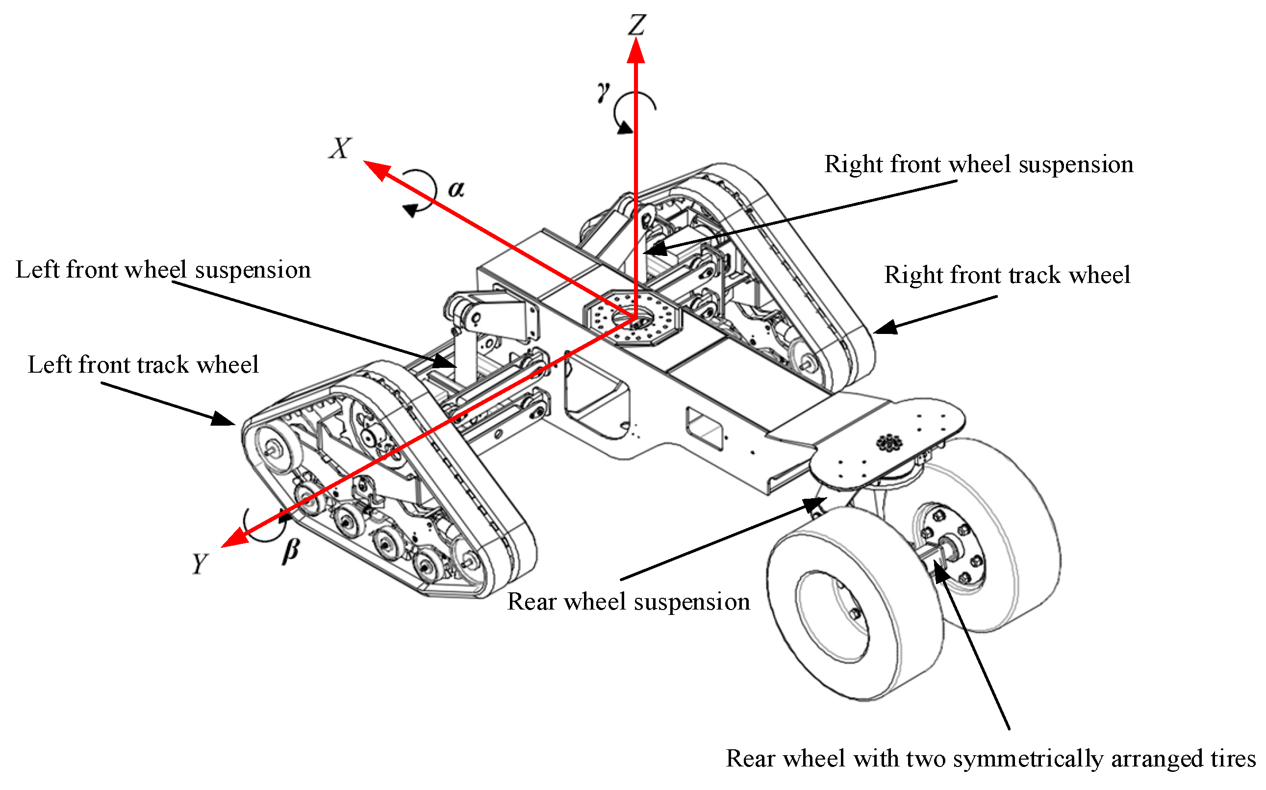
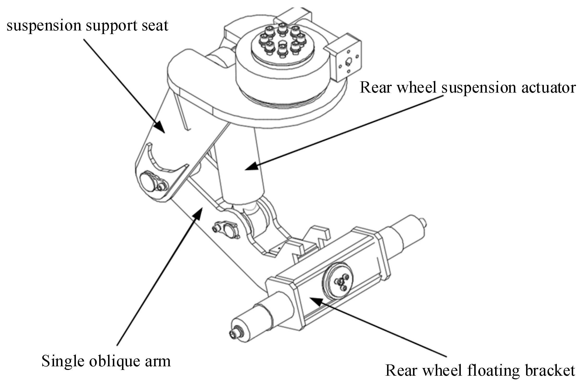
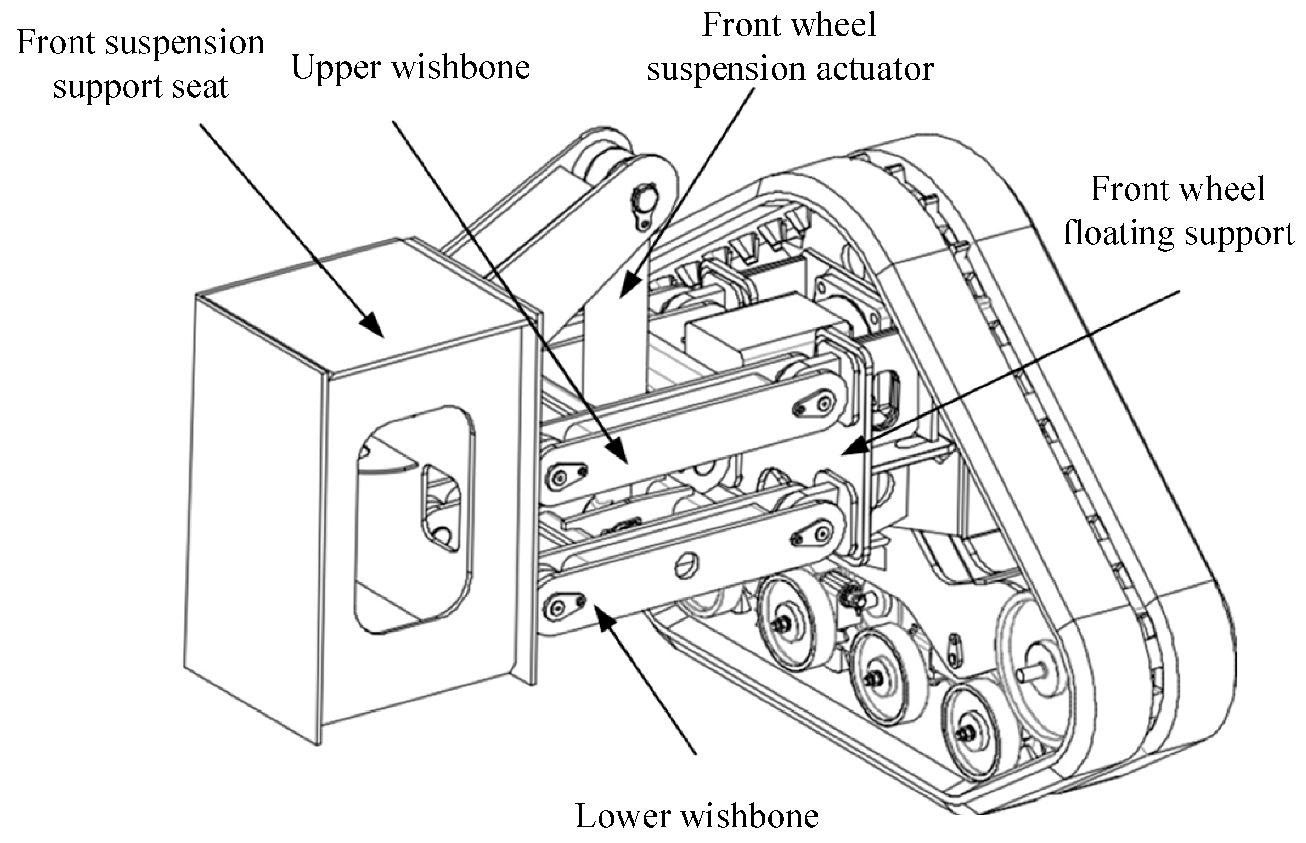
2. The Structure of the Three-Wheeled Chassis Leveling System

The chassis layout of the three-wheeled agricultural robot is shown in Figure 1. Both the front left and front right wheels are tracked, while the rear wheel features a pair of symmetrically arranged dual tires. To ensure effective leveling for the chassis, all three wheels are equipped with independent suspension. The chassis leveling system of the three wheeled agricultural robot utilizes the three-point leveling principle, which controls the horizontal orientation of the chassis by adjusting the height of three support points. This leveling system offers advantages such as a simple structure, simple control strategy, and rapid leveling response. Consequently, it is suitable for agricultural tasks in situations with poor road conditions that require quick leveling.
Firstly, the rear suspension is briefly introduced. Figure 2 illustrates the structure of the rear wheel suspension. This suspension employs a single oblique arm independent suspension. By adjusting the suspension actuator, the relative position between the rear suspension support seat and the single oblique arm can be changed, thus altering the height of the chassis support point from the rear wheel.
The mechanism principle of the rear wheel suspension is shown in Figure 3. The detailed derivation of the mathematical model is provided in Appendix A.
Then, the front suspension structure is briefly introduced. The front suspension of the three-wheeled agricultural robot chassis employs a double-wishbone independent suspension, as shown in Figure 4. The front wheel suspension actuator can adjust the relative position of the front suspension seat and the double wishbone, thereby altering the distance between the chassis support point and the wheel.
Figure 5 shows the mechanism schematic diagram of the front wheel double-wishbone independent suspension. The detailed derivation of the mathematical model is provided in Appendix A.

3. Mathematical Modelling

3.1. Force Model of the Three-Wheeled Chassis

Based on the mechanism principle of the active suspension of the three-wheeled chassis, the force analysis model of the chassis was established, as shown in Figure 6. For the force model, the physical meaning of each variable symbol is described below. Zb represents the vertical displacement of the vehicle body centroid. α and β indicate the roll angle and pitch angle, respectively. ZA1, ZB1, and ZC1 indicate the sprung mass displacement at the left front wheel, right front wheel, and rear wheel suspension, respectively. ZA2, ZB2, and ZC2 represent the wheel displacement of the left front wheel, right front wheel, and rear wheel. wA, wB, and wC indicate the road excitation of each wheel. FA1, FB1, and FC1 indicate the force exerted by the left front wheel, right front wheel, and rear wheel suspension on the chassis. FA2, FB2, and FC2 represent the controllable forces provided by the hydraulic actuators of the left front wheel, right front wheel, and rear wheel suspension. cA, cB, and cC indicate the damping coefficients of the left front wheel, right front wheel, and rear wheel suspension. ksA, ksB, and ksC indicate the spring stiffness of the left front wheel, right front wheel, and rear wheel suspension. ktA, ktB, and ktC indicate the tire stiffness of the left front wheel, right front wheel, and rear wheel. Ms stands for the mass of the vehicle body of the three-wheeled chassis. MA1, MB1, and MC1 represent the sprung mass at the left front wheel, right front wheel, and rear wheel suspension, while MA2, MB2, and MC2 represent the unsprung mass at the left front wheel, right front wheel, and rear wheel suspension. After the force analysis of the chassis, the following formula can be obtained. The vibration model of the chassis can be given by:
M x 2 Z x 2 + k s x ( Z x 2 Z x 1 ) + k t x ( Z x 2 w x ) + c x ( Z x 2 Z x 1 ) + F x 2 = 0 F x 1 + k s x ( Z x 1 Z x 2 ) + c x ( Z x 1 Z x 2 ) F x 2 = 0 M s Z b F A 1 F B 1 F C 1 = 0 ( x = A ,   B ,   C )

3.2. Attitude Model of the Three-Wheeled Chassis

The attitude analysis parameters of the chassis mainly include the body vertical displacement, Zb, pitch angle, β, and roll angle, α. Each wheel of the three-wheeled agricultural robot experiences different road excitations, resulting in different sprung mass displacement of each suspension. The superposition effect of these three different displacement amounts causes changes in the chassis attitude. The relationship between the sprung mass displacement of the three suspensions and the chassis attitude parameters can be expressed as follows:
Z A 1 = l f 2 sin α l bf sin β + Z b
Z B 1 = l f 2 sin α l bf sin β + Z b
where lf is the distance between the two front wheel suspensions, lbf is the distance between the vehicle body centroid and the center of the two front wheel suspensions, and lbr is the distance between the vehicle body centroid and the rear wheel suspension.
The changes in the chassis pitch angle and roll angle reflect the variations in the external moments acting on the vehicle body. The change in pitch angle results from the combined pitching moment acting on the vehicle body, while the change in roll angle is due to the combined rolling moment. Therefore, based on the rigid body rotational dynamics equations, the following two equations can be derived:
M x = I x β = ( F A 1 + F B 1 ) l bf + F C 1 l br
M y = I y α = ( F A 1 F B 1 ) l f 2
where Ix and Iy represent the pitch moment of inertia and the roll moment of inertia, respectively. Mx denotes the pitch moment of the vehicle body and My denotes the roll moment of the vehicle body.

3.3. Single-Wheel Suspension System Model

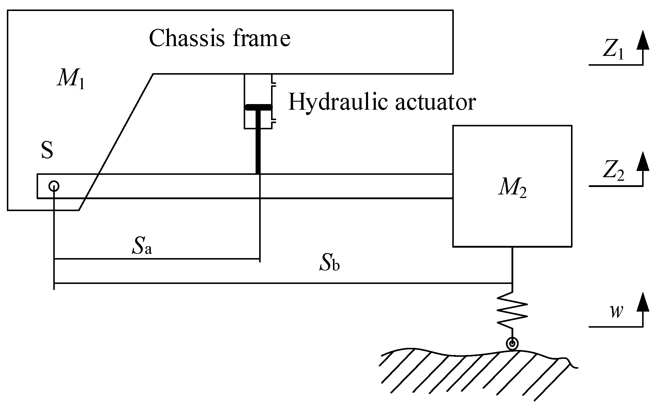
3.3.1. Single-Wheel Suspension Model

The single-wheel suspension model of the chassis of the three-wheeled agricultural robot is shown in Figure 7. In this simplified model, since only one of the A, B, and C suspensions is considered for modeling, the symbols used in the full model in Section 3, such as Mx1 (where x = A, B, C), are simplified to M1 for clarity. Other similar symbols are simplified in the same way.
In this paper, the distances from the hinge point, S, to the hydraulic actuator and the wheel are defined as Sb and Sa, respectively. Thus, the motion equation of the single-wheel suspension model can be derived, as shown in the following equation.
M 1 Z ¨ 1 F 2 + k s ( Z 1 Z 2 ) + c ( Z 1 Z 2 ) = 0 M 2 Z ¨ 2 + k t ( Z 2 w ) + F 2 + k s ( Z 2 Z 1 ) + c ( Z 2 Z 1 ) = 0

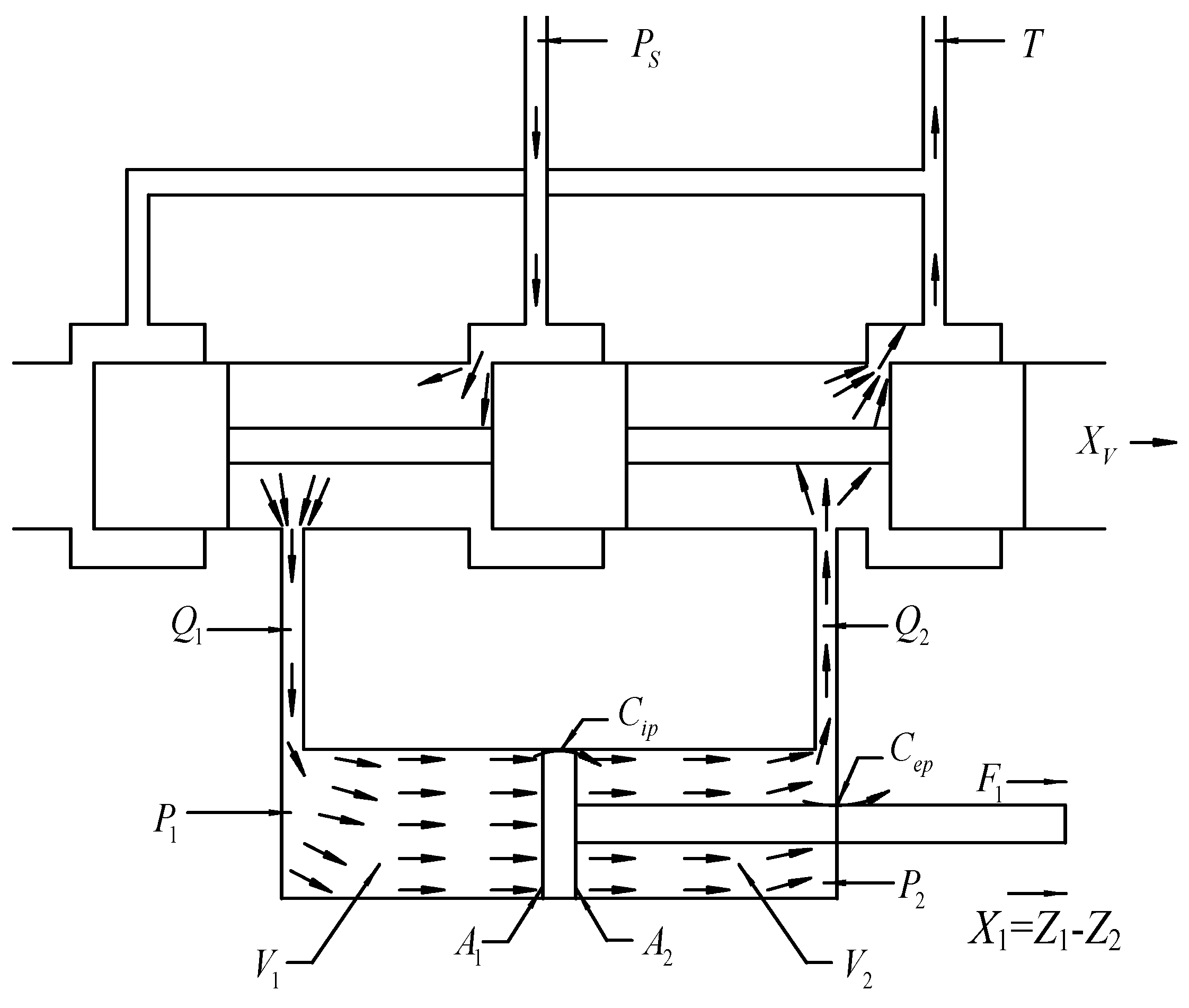
3.3.2. Hydraulic Servo System Model of the Suspension Actuator

The hydraulic actuator system is the primary energy absorption and output component in independent active suspension systems. Its dynamic response performance is a crucial factor affecting the damping and leveling capabilities of the active suspension system. As a nonlinear system, the hydraulic actuator can be simplified to a valve-controlled cylinder system, as illustrated in Figure 8.
Based on the valve flow equation, hydraulic cylinder flow equation, and hydraulic cylinder force balance equation, the state equations for hydraulic system pressures P1 and P2 and suspension displacements Z1 and Z2 are derived as follows (The detailed derivation of the hydraulic servo system model of the suspension actuator is provided in Appendix B):
P ˙ 1 = β e V 1 { C d ω X v 2 ρ [ S ( X v ) P s P 1 + S ( X v ) P 1 ] A 1 ( Z 1 Z 2 ) } P ˙ 2 = β e V 2 { C d ω X v 2 ρ [ S ( X v ) P 2 + S ( X v ) P s P 2 ] A 2 ( Z 1 Z 2 ) }
S ( x ) = { 1 x 0 0 x < 0
Z ¨ 1 = A 1 P 1 A 2 P 2 + k s ( Z 2 Z 1 ) + c ( Z 2 Z 1 ) M 1 Z ¨ 2 = A 2 P 2 A 1 P 1 + k s ( Z 1 Z 2 ) + c ( Z 1 Z 2 ) + k t ( w Z 2 ) M 2
where Xv represents the valve spool displacement, Ps represents the supply pressure, P1 represents the pressure in the rodless chamber, P2 represents the pressure in the rod chamber, ρ represents the fluid density, ω represents the valve port area gradient, Cd represents the flow coefficient of the throttling orifice, V1 represents the volume of the rodless chamber of the hydraulic cylinder, V2 represents the volume of the rod chamber of the hydraulic cylinder, A1 represents the effective piston area of the rodless chamber, A2 represents the effective piston area of the rod chamber, and βe represents the effective bulk modulus.

3.3.3. State Equation of the Single-Wheel Suspension

Choose the following state variables: x 1 = Z 1 Z 2 , x 2 = Z ˙ 1 , x 3 = Z 2 , x 4 = Z ˙ 2 , x 5 = w . Based on the dynamics equations of the single-wheel suspension system, the state-space equations can be derived as follows:
x ˙ 1 = x 2 x 4 x ˙ 2 = u ˜ M 1 x ˙ 3 = x 4 x ˙ 4 = 1 M 2 [ K ( x 3 x 5 ) + u ˜ ] x ˙ 5 = 2 π f 0 w ( t ) + 2 π G 0 v r ( t )
Taking the suspension actuator control force as the virtual control input, u ˜ , and selecting the vertical acceleration, Z ¨ 1 , of the vehicle body, the suspension dynamic stroke ( Z 1 Z 2 ), and the tire dynamic displacement ( Z 2 w ) as the system outputs, Equation (10) can be rewritten as follows:
X ˙ = A X + B U ˜ + G r Y = C X + D U ˜
where X represents the state variables, r represents the disturbance input, and A, B, C, D, and G represent the coefficient matrices.
A = [ 0 1 0 1 0 0 0 0 0 0 0 0 0 1 0 0 0 K M a 0 K M a 0 0 0 0 2 π f 0 ] B = [ 0 1 M b 0 1 M a 0 ] T C = [ 1 0 0 0 0 0 0 0 0 0 0 0 1 0 1 ] D = [ 0 1 M b 0 ] T G = [ 0 0 0 0 2 π G 0 v ] T

4. Chassis Leveling Control

The horizontal stability performance of the chassis in a three-wheeled agricultural robot significantly impacts the overall work efficiency, operational safety, and precision of the machine during agricultural tasks. In terms of ride smoothness, the agricultural robot doesn’t need to consider ride comfort; the main goal is to reduce mechanical wear. Therefore, for the chassis attitude control of the three-wheeled agricultural robot, priority should be given to the leveling performance, while also considering the control performance smoothness. Considering the need for chassis attitude control, this paper introduces a new leveling method: a stepwise leveling method based on an adaptive dual-loop composite control strategy (ADLCCS-SLM).
Firstly, in terms of overall machine attitude control, this paper proposes a rapid leveling method suitable for three-wheeled chassis, referred to in this paper as the stepwise leveling method (SLM). The SLM achieves the vehicle’s leveling goal by adjusting the vehicle suspension in stages, rather than adjusting all the suspensions simultaneously. Specifically, the SLM requires only the pitch and roll angle data of the chassis. By adjusting the minimum number of suspensions, gradually adjusting one or two suspensions, the leveling objective can be achieved. The simplicity and efficiency of this method lie in its incremental approach to adjustments, rather than making simultaneous adjustments to all suspensions. Compared to traditional suspension control methods, the SLM avoids the complex interactions between suspension components that occur when various suspension mechanisms work together. By gradually optimizing adjustments, it is possible to more effectively achieve the vehicle’s balanced state, while also simplifying the design and implementation process of the control system.
In terms of suspension system control, this paper proposes a new method called the adaptive dual-loop composite control strategy (ADLCCS). This strategy employs an inner and outer dual-loop composite control approach, with key control parameters adjusted using an improved adaptive genetic algorithm (IAGA) to adapt to different road conditions and optimize chassis leveling performance. The dual-loop control combines the advantages of both inner and outer loop controls. The outer loop utilizes the linear quadratic Gaussian model (LQG) to derive the optimal virtual control law, effectively enhancing the system’s robustness and response speed. The inner loop employs the backstepping algorithm to handle nonlinear terms, providing the capability to manage complex nonlinear systems. IAGA is used to select the optimal variable parameter combinations for the inner and outer loops under different working conditions, allowing for adaptive adjustments based on actual road conditions, thereby improving the system’s adaptability and leveling performance. The leveling control logic diagram of the three wheeled chassis is shown in Figure 9.

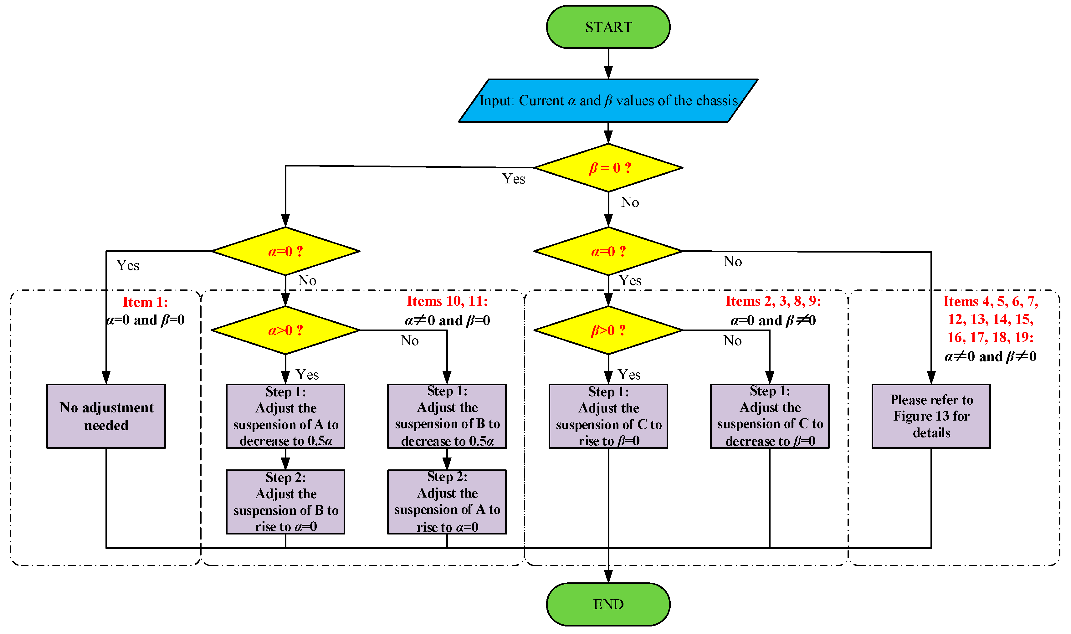
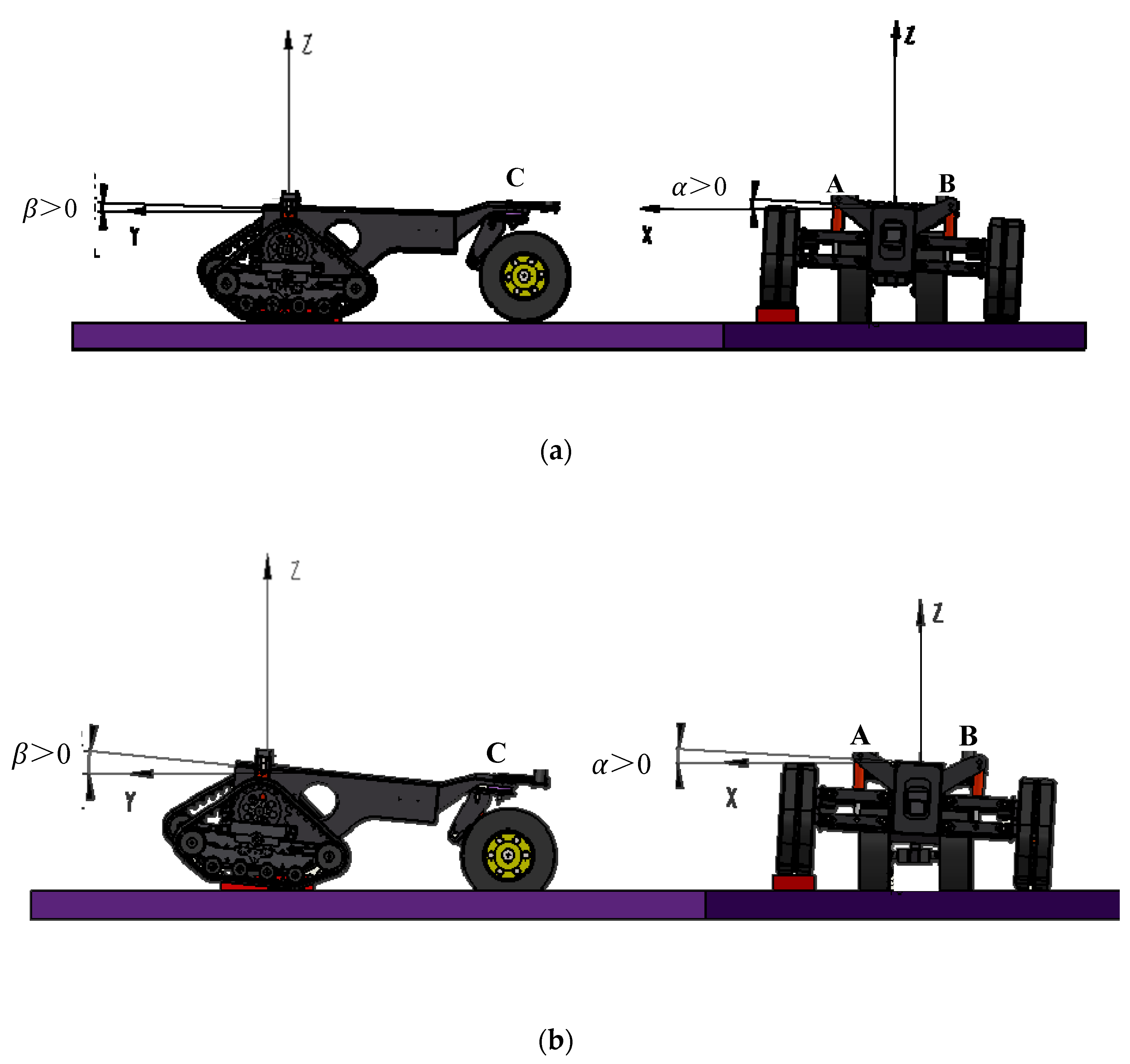
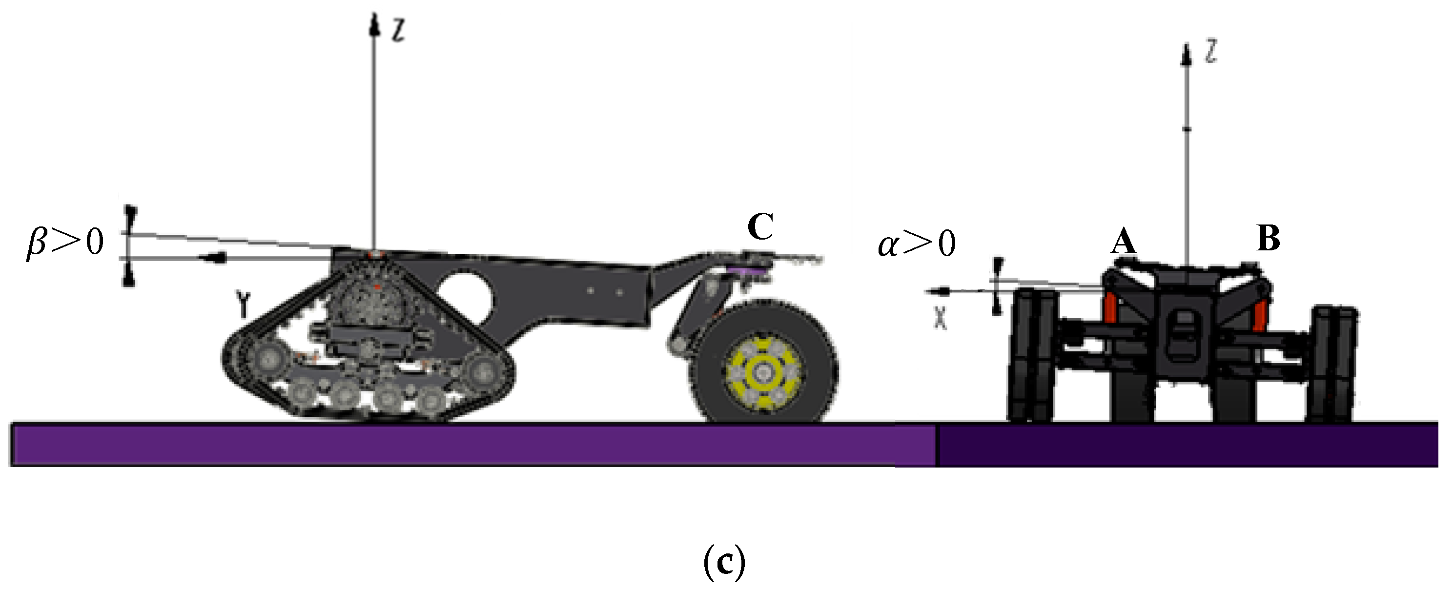
4.1. Chassis Stepwise Leveling Method

Figure 10 illustrates the coordinate system diagram of the three-wheeled chassis. Points A, B, and C represent the support points of the left front suspension, right front suspension, and rear suspension, respectively. OXYZ is the horizontal reference coordinate system, which only translates relative to the absolute coordinate system. OX1Y1Z1 is the rotational coordinate system, which rotates with the vehicle body relative to the horizontal reference coordinate system, OXYZ. The angle of rotation around the X-axis is the roll angle, α, and the angle of rotation around the Y-axis is the pitch angle, β. Both coordinate systems share the same origin, O, located at the midpoint of the AB line segment. The proposed stepwise leveling method sets the chassis reference point at the origin, O, instead of the centroid, simplifying the control process and increasing the speed of leveling.
The chassis attitudes of the three-wheeled agricultural robot during operation were analyzed and classified based on the surface excitations experienced by each wheel. In the end, 19 different chassis attitudes were identified, as shown in Table 2.
(1)
When the chassis maintains a level attitude while moving, α = 0 and β = 0, as shown in item 1 of the table.
(2)
When only one wheel is subjected to road excitation, the chassis has six attitudes, which are considered the basic attitudes of the chassis, as shown in items 2 to 7.
(3)
By combining any two of the aforementioned six basic chassis attitudes and then excluding the combinations that result in the horizontal attitude, an additional 12 chassis attitudes can be derived, as shown in items 8 to 19.
It should be noted that in the table, ΔA, ΔB, and ΔC represent the road excitations experienced by the wheels corresponding to the chassis support points A, B, and C, respectively. The values in the table are not the actual road excitation values but indicate three states of road excitation: 0 indicates no excitation, 1 indicates upward road excitation, and −1 indicates downward road excitation.
To simplify the process of recognizing chassis attitudes, this paper classifies 19 types of chassis attitude into five categories based on the angles α and β: ① α = 0 or β = 0; ② α > 0, β > 0; ③ α > 0, β < 0; ④ α < 0, β > 0; ⑤ α < 0, β < 0. In Table 2, these five categories are marked with gold, yellow, brown, green, and blue backgrounds, respectively. Based on the characteristics of these five categories, a rapid leveling method applicable to all five types of attitudes, called the stepwise leveling method, is proposed. This method involves first adjusting the relatively flexible rear wheel suspension, followed by the front wheel suspension. By adjusting one or two suspensions in a stepwise manner, the leveling goal can be achieved. This method features a small number of suspension adjustments, high precision in phased leveling, and a simple leveling strategy, making it suitable for three-wheeled chassis. The basic principles of the stepwise leveling method will be introduced next.
The first category of chassis attitudes (α = 0 or β = 0) includes seven forms, as indicated by items 1, 2, 3, 8, 9, 10, and 11 in Table 2. Excluding item 1, the remaining six chassis attitudes require adjustment of only one angle, making the leveling process relatively simple. The control logic flowchart for their leveling process is shown in Figure 11.
When α ≠ 0 and β ≠ 0, the chassis attitudes fall into categories 2 to 5, which are more complex and comprise 12 forms (as indicated by items 4, 5, 6, 7, 12, 13, 14, 15, 16, 17, 18, and 19 in Table 2). The following text will detail their leveling principles. The control logic flowchart for their leveling process is shown in Figure 12. First, determine whether the rear wheel suspension needs adjustment based on the condition specified in Equation (13).
l AB sin | α | 2 = l o c sin | β |
If α and β satisfy this angular relationship, the rear wheel suspension does not need to be adjusted. Instead, adjust one of the front wheel suspensions to raise or lower the corresponding support point. The adjustment height, Δ h , for the support point is calculated using Equation (14).
Δ h = sgn α · sgn β · l AB sin | α |
If Δ h > 0 , adjust the left front wheel suspension. The direction of the suspension adjustment is determined by the sign of α (sgn(α)): if sgn(α) is positive, the suspension adjusts downward; if sgn(α) is negative, the suspension adjusts upward. If Δ h < 0 , adjust the right front wheel suspension, with the direction of adjustment similarly determined by sgn(α): if sgn(α) is positive, the suspension adjusts upward; if sgn(α) is negative, the suspension adjusts downward.
If α and β do not satisfy this angular relationship, the rear wheel suspension must be adjusted first to raise or lower the support point C by Δh. The calculation for Δh is given by Equation (15).
Δ h = sgn β · l o c sin | β | sgn α · l AB sin | α | 2
Δh > 0 indicates that the support point C should be raised; Δh < 0 indicates it should be lowered. After this, adjust one of the front wheel suspensions according to Equation (14).
Taking the second category of chassis attitudes (α > 0, β > 0) as an example, the paper will introduce the principles of the stepwise leveling method. According to Table 2, the second category of chassis attitudes includes the three forms indicated by items 5, 14, and 16, as shown in Figure 13.
First, determine whether the rear wheel suspension needs adjustment. If α and β satisfy Equation (13), no adjustment to the rear wheel suspension is necessary; otherwise, adjustment is required.
When α and β satisfy Equation (13), specifically β = sin 1 ( l O A l O C · sin α ) , no adjustment to the rear wheel suspension is necessary. Instead, adjust the left front wheel suspension to lower support point A by Δ h 2 . Δ h 2 is calculated as:
Δ h 2 = l AB · sin α
When α and β do not satisfy Equation (13), specifically β sin 1 ( l O A l O C · sin α ) , first adjust the rear wheel suspension to raise support point C by Δ h 2 . Then, adjust the left front wheel suspension to lower support point A by Δ h 2 . Δ h 2 is calculated as:
Δ h 2 = l OC · sin β l AB · sin α 2
The proposed stepwise leveling method is specifically designed for three-wheeled chassis, integrating the unique structure and power distribution characteristics of three-wheeled vehicles. By individually adjusting the front two wheels and the rear wheel, it better meets the practical requirements of three-wheeled vehicles. Traditional leveling methods adjust all suspensions simultaneously based on the chassis’ pitch and roll angles, which leads to dynamic coupling issues among the suspensions. In contrast, the stepwise leveling approach not only resolves the complex control challenges arising from complex interactions between suspension components but also streamlines the implementation process of leveling control.

4.2. Adaptive Dual-Loop Composite Control Strategy (ADLCCS)

To enhance the control performance of suspension actuators, this paper proposes a new control strategy, namely, the adaptive double-loop composite control strategy (ADLCCS). First, a composite controller combining inner-loop and outer-loop control was designed. The outer loop uses the linear quadratic Gaussian (LQG) model to obtain the optimal virtual control law, while the inner loop employs the backstepping algorithm, which excels in handling nonlinear systems, to address the nonlinear components of the system. The structural principle of the composite controller is shown in Figure 14. Then, an improved IAGA was introduced to optimize the key control variables of the inner and outer loop controllers, in order to enhance the adaptability of the composite controller in actual road conditions.

4.2.1. Design of the Outer-Loop Controller

The design of the LQG optimal controller adheres to the separation principle and can be divided into two main parts: firstly, optimal state estimation is conducted using a Kalman filter; secondly, the optimal control law is derived based on optimal control theory.
During vehicle operation, certain state variables such as vertical ground displacement are difficult to measure directly. Although previous optimal controllers typically assume a full-state feedback system, acquiring these variables directly often poses a challenge in practice. Therefore, employing a Kalman filter for state estimation becomes essential, using optimal estimation methods to predict key state variables like vertical displacement. Let the measurable state output equation be:
Y c ( t ) = C m X ( t ) + v ( t )
where Cm represents the measurement matrix and v(t) represents the measurement noise.
C m = [ 1 0 0 0 0 0 1 0 0 0 0 0 0 1 0 ]
Assume that the model noise and measurement noise are uncorrelated and satisfy the following relationship:
E [ w ( t ) w ( t + τ ) ] = R 1 δ ( t ) E [ v ( t ) v ( t + τ ) ] = R 2 δ ( t )
According to the Kalman filter equation, the following equation can be obtained:
X ^ ˙ ( t ) = A X ^ ( t ) + B U ˜ ( t ) + L [ Y c ( t ) C m X ^ ( t ) ] = ( A L C m ) X ^ ( t ) + B U ˜ ( t ) + L Y c ( t )
The gain matrix of the optimal state observer is:
L = P ^ C m T R 2 1
P ^ is the solution to the following state Riccati equation.
A P ^ + P ^ A T P ^ C m T R 2 1 C m P ^ + G R 1 G T = 0
After estimating the state variables, the next step is to design the optimal controller. Analyzing Equations (11), (12), and (20), it becomes apparent that the system is a typical linear time-invariant system, meeting the basic criteria for optimal controller design. Tire displacement, suspension travel, and the vehicle body’s vertical acceleration are selected as evaluation metrics. Based on these, the system’s objective function is constructed, as shown in the following equation.
J = lim T 1 T 0 T [ q 1 ( Z 1 Z 2 ) 2 + q 2 Z ¨ 1 2 + q 3 ( Z 2 w ) 2 ] d t
Let Q 0 = [ q 1 q 2 q 3 ] be the weighting function matrix; thus, Equation (24) can be rewritten as follows:
J = lim T 1 T 0 T ( X T Q X + U ˜ T R U ˜ + 2 X T N U ) d t
where Q represents the state weighting matrix, and its expression is Q = C T Q 0 C ; R represents the control weighting matrix, and its expression is R = r = 1 M 1 2 ; N represents the correlation weighting matrix, and its expression is N = C T Q 0 D .
Q = [ q 1 0 0 0 0 0 0 0 0 0 0 0 q 3 0 q 3 0 0 0 0 0 0 0 q 3 0 q 3 ]
According to optimal control theory, the optimal control law for state feedback that minimizes the performance index is:
U ˜ = K s X ^
The feedback gain matrix is:
K s = R 1 B T P
P is the solution to the following state Riccati equation.
P A + A T P P B R 1 B T P + Q n = 0

4.2.2. Design of the Inner Loop Controller

In the inner loop control, the backstepping algorithm is employed to compensate for the nonlinearities in the hydraulic actuator system. To meet performance requirements, the control input, u, must approximate the virtual control, u ˜ , thereby achieving optimal control output. Additionally, by introducing two extra state variables, x6 = P1 and x7 = P2, the following equations can be obtained:
x ˙ 6 = β e V 1 { C d ω X v 2 ρ [ S ( X v ) P s x 6 + S ( X v ) x 6 ] A 1 ( x 2 x 4 ) } x ˙ 7 = β e V 2 { C d ω X v 2 ρ [ S ( X v ) x 7 + S ( X v ) P s x 7 ] A 2 ( x 2 x 4 ) }
Define the error variable z as shown in the following equation:
z = u u ˜
Construct the Lyapunov function and its derivative, with the specific expressions being V = 1 2 z 2 and V ˙ = z z ˙ , respectively. Assuming the control input is XV, to ensure stability of the control system, the actual control law selected is:
X v = A 1 D 1 ( x 2 x 4 ) + D 2 A 2 ( x 2 x 4 ) + u ˜ ˙ k z D 1 H 1 + D 2 H 2
where
D 1 = A 1 β e V 1 D 2 = A 2 β e V 2 H 1 = C d ω 2 ρ [ S ( X v ) P s x 6 + S ( X v ) x 6 ] H 2 = C d ω 2 ρ [ S ( X v ) x 7 + S ( X v ) P s x 7 ]
By choosing k > 0, ensure that V ˙ = z z ˙ = k z 2 0 , thereby gradually stabilizing the error, which means the inner loop control strategy achieves asymptotic stability.

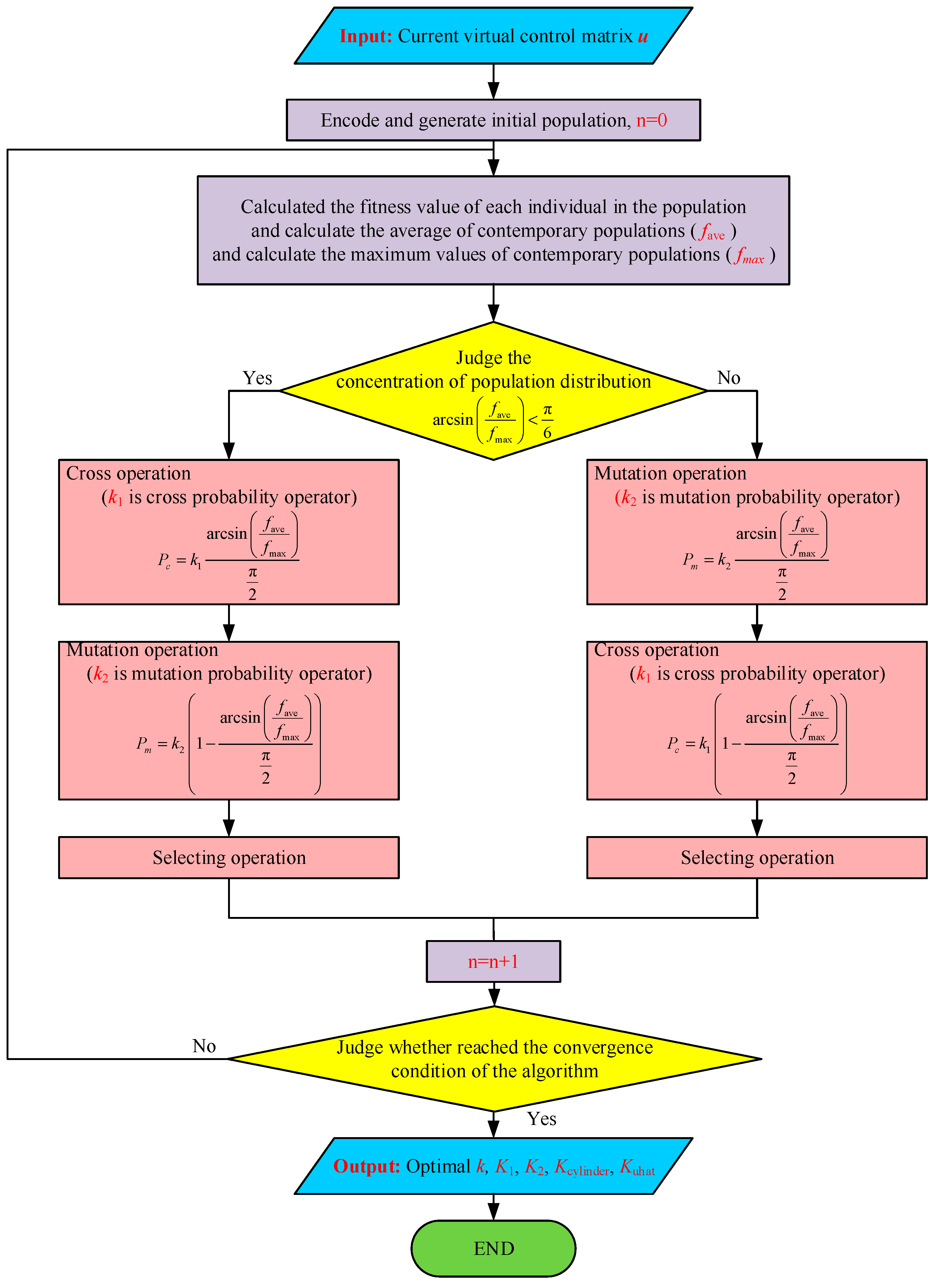
4.2.3. Adaptive Optimization of Control Parameters

According to Equation (32), k, as an adjustable gain in the control rate, significantly affects the rate at which the control input, u, approximates the virtual control, u ˜ , and the ultimate stabilization time in the inner loop control. The actual control rate, Xv, which corresponds to the valve opening, can lead to severe hydraulic cylinder pressure fluctuations and resultant hydraulic system shocks and pipeline vibrations if k is too high. Conversely, if k is too low, it can prolong the stabilization time of the inner loop control, adversely affecting the performance of active suspension control. Therefore, by using an optimization algorithm that considers the rate of change in the virtual control, u ˜ , selecting the optimal k value for the current conditions can achieve the best control performance.
First, establish the objective function for the inner loop control. Considering the rate of change in the virtual control variable, u ˜ , along with the adjustment rate of the error variable, z ˙ , and the current error amount, z, the system’s objective function, Jk, is constructed as:
J k = min f = 0 T [ K 1 · z 2 + K 2 · ( z ˙ ) 2 ] d t
where K1 is the error weight and K2 is the weight for the error adjustment rate. Different combinations of K1 and K2 reflect the system’s focus on stability and speed in inner loop control under various control modes.
Considering the response characteristics of hydraulic systems, using only the control force output by the hydraulic actuator as the input for optimal control could lead to excessive fluctuations in the solved virtual control variable due to pressure variations in the hydraulic system. To minimize the impact of these pressure fluctuations, this paper incorporates both the current output control force of the hydraulic actuator and the solved virtual control variable, u ˜ , as inputs for optimal control. Additionally, it utilizes variable parameter weights, Kcylinder and Kuhat, as input weights for the current output control force and the virtual control variable, respectively.
Based on the analysis of key parameters for the inner and outer loop controllers discussed previously, it is clear that the controller contains five critical optimizable variables: (1) the adjustable gain, k, for the valve opening, Xv; (2) the error weight, k1, and the error adjustment rate weight, k2, for the virtual control quantity, u ˜ , in the inner loop’s control; (3) the control force input weight, Kcylinder, and virtual control variable input weight, Kuhat, for the hydraulic actuator in the outer loop’s control. The different combinations of these five control variables will affect the chassis leveling performance under various operating conditions, necessitating the use of optimization algorithms to determine the optimal variable combinations for different scenarios.
This paper employs an improved adaptive genetic algorithm to overcome the shortcomings of traditional genetic algorithms. These improvements include assessing the degree of population aggregation and adjusting adaptive crossover mutation probabilities.
Figure 15 shows the flowchart of the adaptive genetic algorithm designed in the paper. The specific steps of the optimization process are as follows:
(1)
Take the change matrix of the virtual control variable, u ˜ , as the input, generate the initial optimization population, and perform encoding.
(2)
Use the objective function, Jk, to evaluate the fitness of each individual in the current population and calculate the average fitness (fave) and the maximum fitness (fmax) of the population.
(3)
Analyze the dispersion of the population to determine the evolutionary direction of the population: if the distribution is dispersed, proceed to step (4); if the distribution is concentrated, proceed to step (5).
(4)
In the case of a dispersed population distribution, generate a new generation of individuals: first perform crossover operations, then perform mutation operations, and finally complete the selection process.
(5)
In the case of a concentrated population distribution, generate a new generation of individuals: first perform mutation operations, then perform crossover operations, and finally complete the selection process.
(6)
Evaluate whether the current population meets the aggregation requirements: if it does, proceed to step (7); if not, return to step (2) for re-evaluation.
(7)
After optimization, output the optimal values of k, K1, K2, Kcylinder, and Kuhat corresponding to the change matrix of the current virtual control variable, u ˜ .
To better utilize the roles of crossover and mutation processes across various population dispersion levels, this paper adopts the nonlinear adaptive calculation formulas for crossover probability and mutation probability in IAGA, as given in Equations (35) and (36).
P c = { k 1 arcsin ( f ave f max ) π 2     , arcsin ( f ave f max ) < π 6 k 1 ( 1 arcsin ( f ave f max ) π 2 ) , arcsin ( f ave f max ) π 6
P m = { k 2 ( 1 arcsin ( f ave f max ) π 2 )   , arcsin ( f ave f max ) < π 6 k 2 arcsin ( f ave f max ) π 2     , arcsin ( f ave f max ) π 6
The arcsin(fave/fmax) ratio serves as a criterion for assessing the dispersion level of a population, determined by the population’s average fitness, fave, and the maximum fitness, fmax.
When arcsin(fave/fmax) < π/6, it indicates that the population is relatively dispersed. The smaller the value compared to π/6, the easier it is to conclude that the population is dispersed, exhibiting high diversity and richness. Under these conditions, adaptively increase the crossover probability to ensure thorough gene exchange and the evolution of superior new individuals; concurrently, adaptively decrease the mutation probability to minimize the risk of deteriorating high-quality individuals and accelerate convergence.
When arcsin(fave/fmax) ≥ π/6, it suggests that the population is relatively concentrated. The larger the value compared to π/6, the more it indicates a concentrated population distribution with less diversity and a more homogeneous population. In this scenario, adaptively decrease the crossover probability to prevent disruption of existing high-quality genes; simultaneously, increase the mutation probability to enhance the population’s global search capabilities and avoid being trapped in local optima.

5. Simulation Study

5.1. Simulation Setup

The simulation model was built based on MATLAB/Simulink. Simulations for chassis leveling were conducted using a convex road surface for road excitations. The effectiveness of the ADLCCS-SLM proposed in this paper is validated by comparison with passive suspension and PID-controlled active suspension. The PID-controlled active suspension in the simulation adopts the traditional multi-suspension linkage leveling method, which differs from the stepwise leveling method proposed in this paper. In the following text, this traditional leveling method based on PID control will be referred to as the PID control method. The main simulation parameters are shown in Table 3. The simulation structure diagram is shown in Figure 16.
The simulation adopts a convex pavement for the road disturbance, and the road model formula is as follows:
z r = { h 2 [ 1 cos ( 2 π v L t ) ] , 0 t < L / v 0 , t L / v
where h is the height of the convex pavement, h = 0.2 m; L is the length of the convex pavement, L = 2.5 m; and v is the vehicle speed, v = 10 km·h−1.

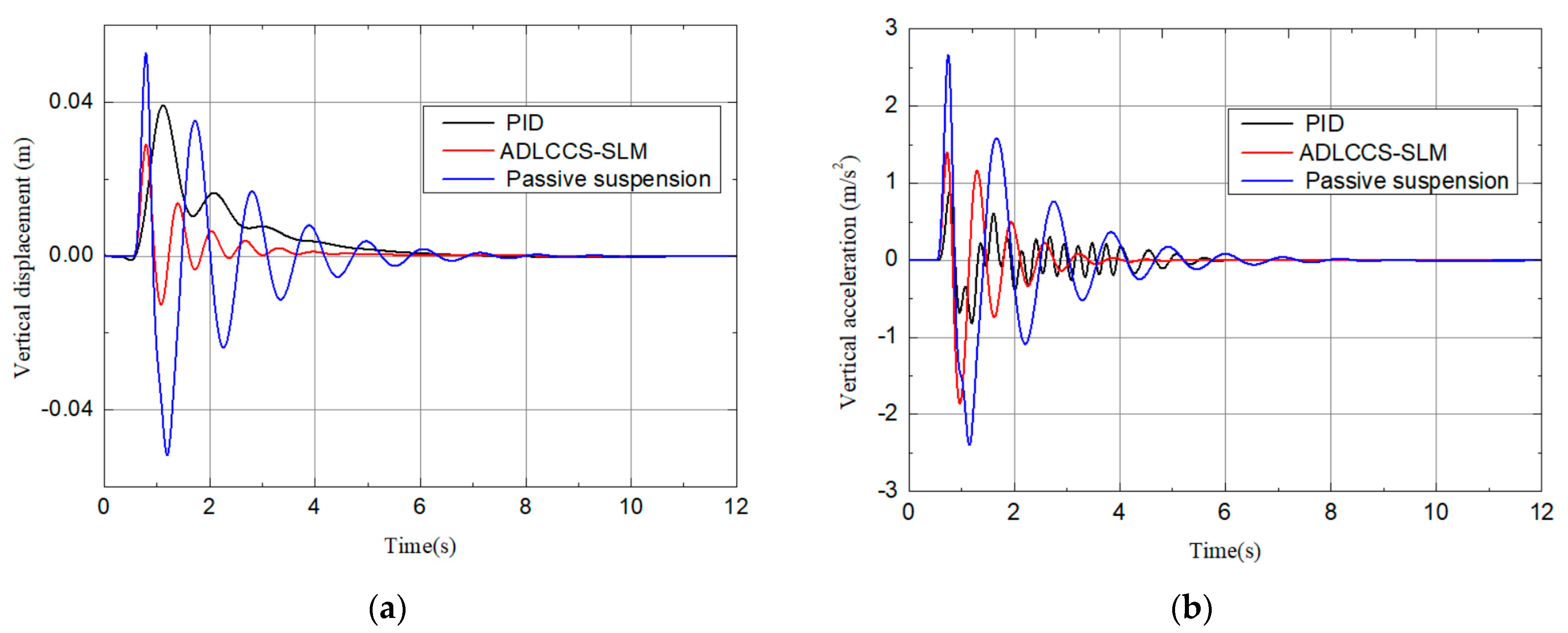
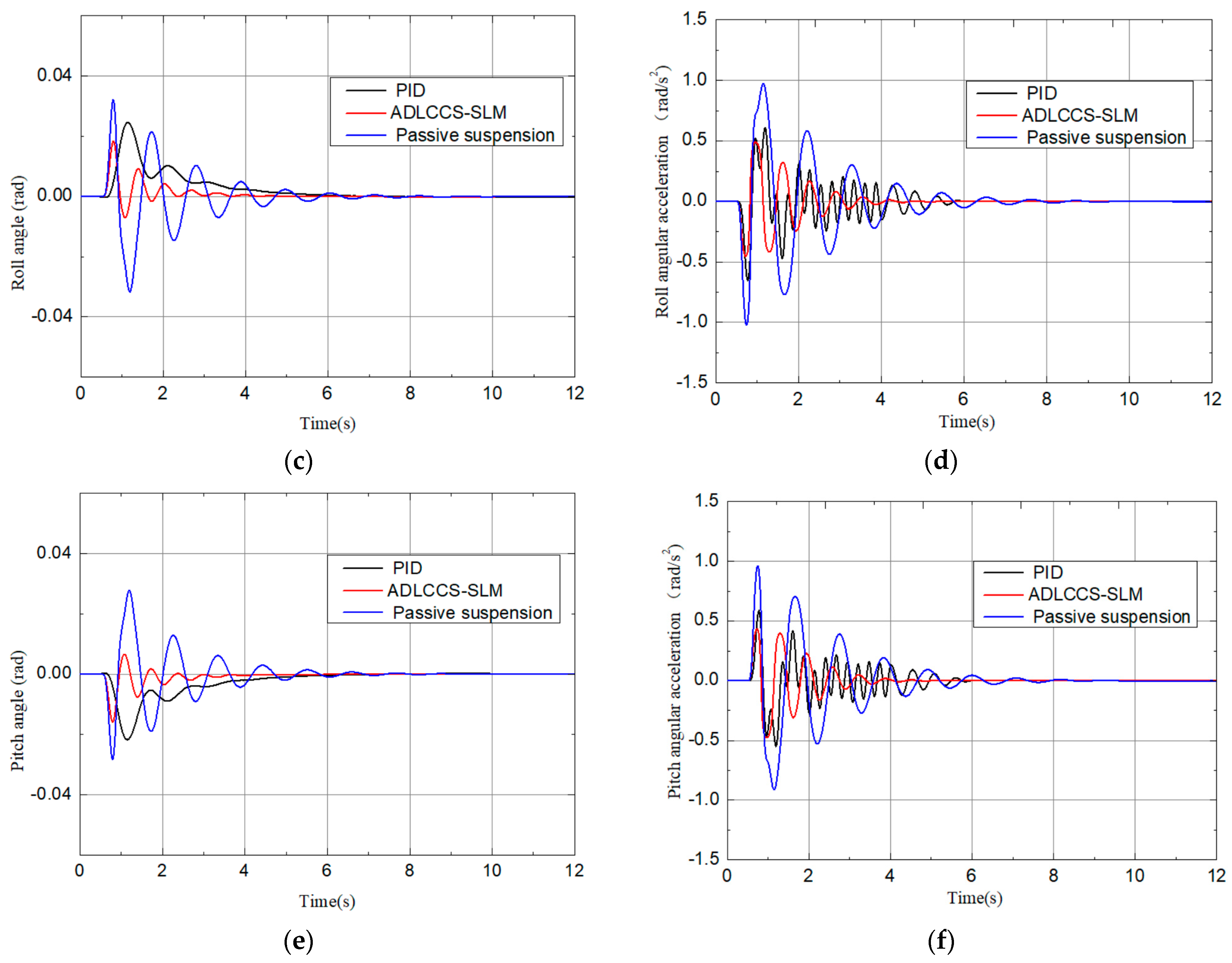
5.2. Comparison with Baseline Methods

The simulation results are shown in Figure 17. During the suspension leveling process, two important performance indicators are the peak values of vertical displacement, the pitch angle, and the roll angle and the leveling time. The peak values refer to the maximum deviation of the chassis’ center of mass, pitch angle, and roll angle from their initial positions during leveling. This indicator reflects the stability and vibration amplitude of the chassis during the leveling process; the smaller the peak values, the better the stability of the chassis. Leveling time refers to the time required from the start of the suspension leveling to the point where the chassis reaches a stable, level state. The shorter the leveling time, the faster the system’s response speed, indicating higher efficiency of the suspension leveling system.
Under the excitation of a convex road, the chassis based on passive suspension experiences large fluctuations in vertical displacement, the pitch angle, and the roll angle. In contrast, both the traditional PID-controlled active suspension and the ADLCCS-SLM-controlled active suspension exhibit significant leveling effects, with the ADLCCS-SLM-controlled chassis showing smaller fluctuations in vertical displacement, the pitch angle, and the roll angle. The leveling time for the passive suspension is 8 s; for the PID-controlled active suspension it is 6 s; and for the ADLCCS-SLM-controlled active suspension it is only 4 s. Clearly, the ADLCCS-SLM achieves a faster leveling speed. Table 4 shows the peak values of chassis attitude parameters for the passive suspension, PID-controlled active suspension, and ADLCCS-SLM-controlled active suspension. Compared to the passive suspension, the peak values of vertical displacement, the pitch angle, and the roll angle for the chassis with traditional PID control are reduced by 22.46%, 22.45%, and 22.41%, respectively, while those for the chassis with ADLCCS-SLM control are reduced by 44.84%, 42.79%, and 44.1%, respectively. Overall, compared to the passive suspension and the PID-controlled active suspension, the ADLCCS-SLM-controlled active suspension performs better in leveling the chassis attitude.

5.3. Discussion

In terms of acceleration suppression, both the PID-controlled active suspension and the ADLCCS-SLM-controlled active suspension perform significantly better than the passive suspension. Comparing the two active suspensions, the PID-controlled suspension excels in vertical acceleration suppression, while the ADLCCS-SLM-controlled suspension slightly outperforms in roll angle acceleration and pitch angle angular velocity suppression. Overall, ADLCCS-SLM shows a significant improvement in chassis smoothness control compared to the passive suspension but no notable improvement over traditional PID control. As mentioned earlier, the chassis control of the three-wheeled agricultural robot prioritizes leveling performance, with smoothness control being a secondary consideration. Therefore, the performance of ADLCCS-SLM in smooth control also meets application requirements.

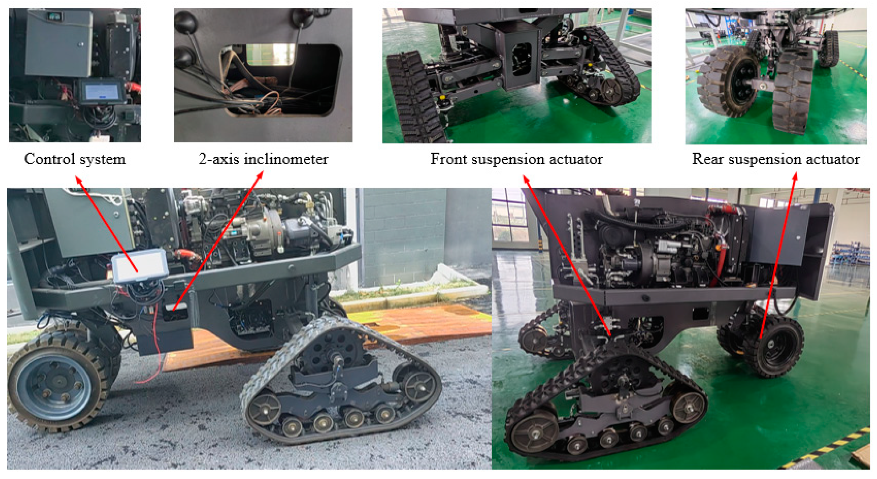
6. Test Verification
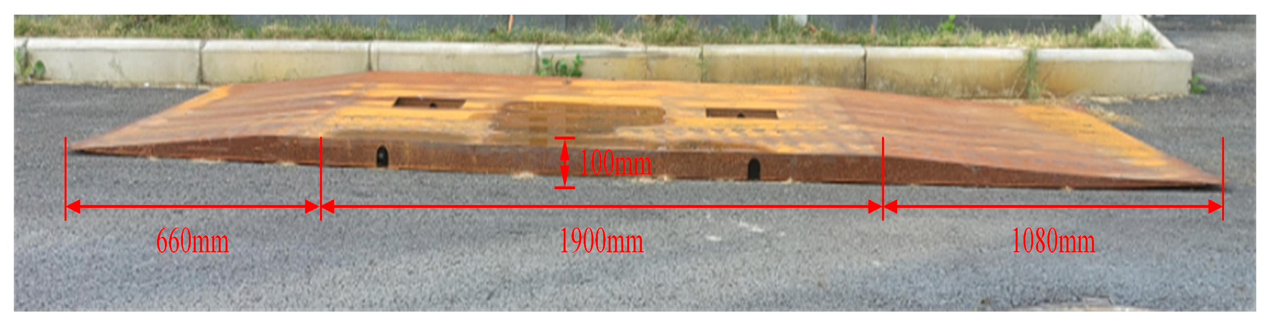
6.1. Test Setup

The experimental prototype of the three-wheeled agricultural robot is shown in Figure 18. During testing, its speed was set to 1 km/h, which is the typical operating speed of the prototype. Figure 19 illustrates the convex test road, which is an arched one-sided bridge. Since the test prototype employs an active suspension system, only the PID-based multi-suspension linkage leveling method and ADLCCS-SLM were tested in the leveling method comparison.

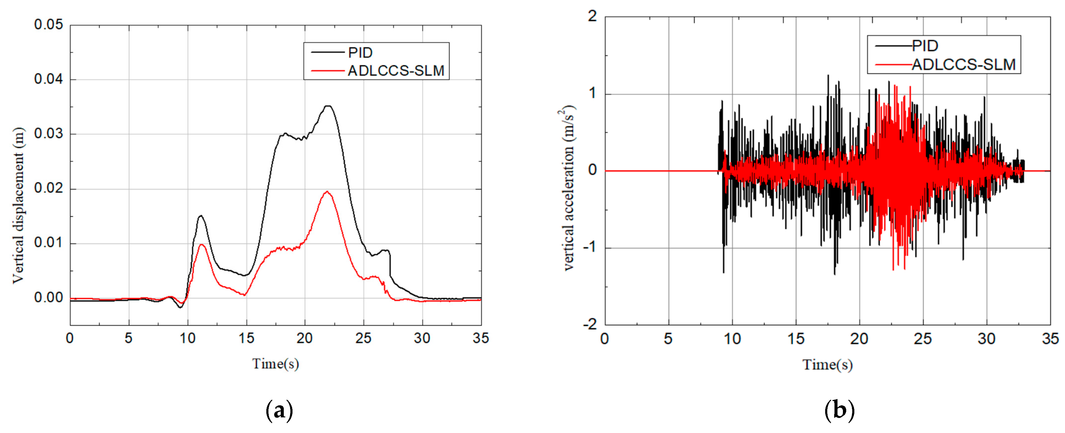
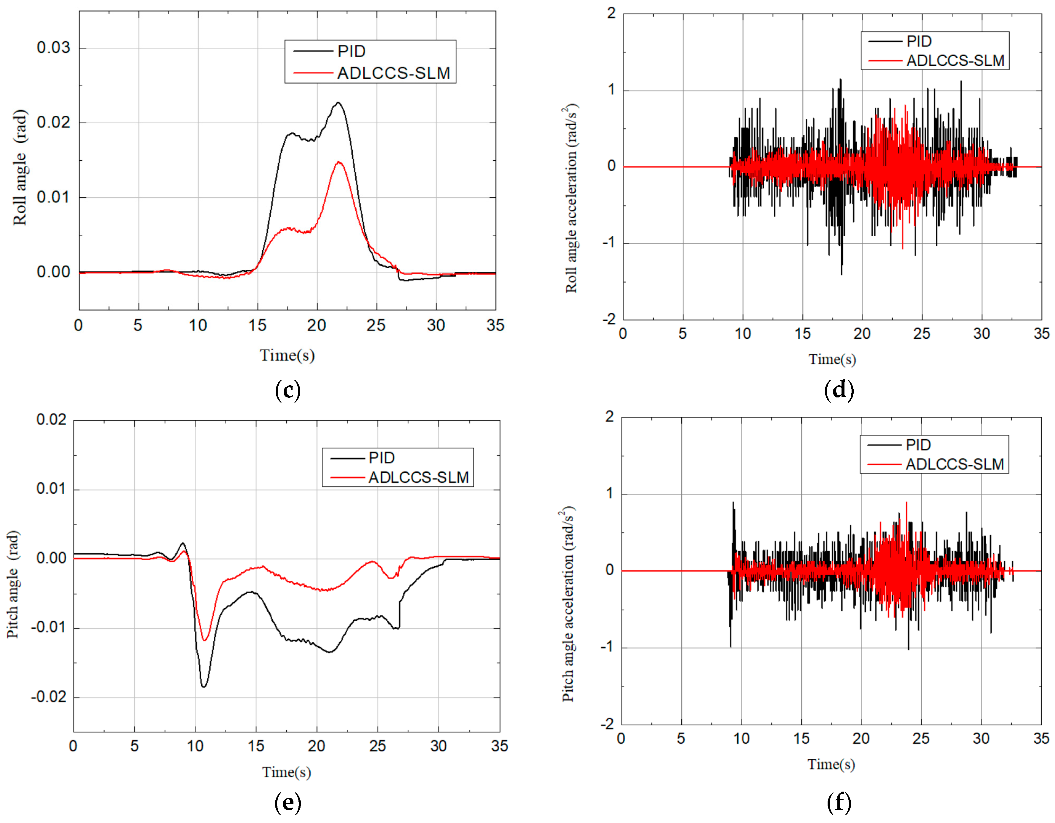
6.2. Comparison with Baseline Methods

The response curves for vertical displacement, the pitch angle, the roll angle, and their accelerations of the test prototype under convex road excitation are shown in Figure 20. From Figure 20a,c,e, it can be seen that the fluctuations in vertical displacement, the roll angle, and the pitch angle of the vehicle body are smaller under ADLCCS-SLM control, indicating that the leveling effect of the active suspension controlled by ADLCCS-SLM is significantly better than that of the traditional PID-controlled active suspension. Table 5 shows the peak values of vertical displacement, the roll angle, and the pitch angle for both leveling control methods. Compared to the traditional PID-based multi-suspension-linked leveling control method, the peak values of vertical displacement, roll angle, and pitch angle under ADLCCS-SLM control are reduced by 42.9%, 31.8%, and 33.3%, respectively. These results indicate that the leveling effect of ADLCCS-SLM is effective.
From Figure 20b,d,f, it can be seen that the peak values of vertical acceleration of the chassis under ADLCCS-SLM control are similar to those under PID control. However, for roll and pitch acceleration suppression, the peak acceleration values under ADLCCS-SLM control are slightly lower than those under PID control. This indicates that ADLCCS-SLM performs slightly better than PID in ride comfort control, though the improvement is limited. This result is consistent with the simulation results. The main reason is that the control objective of ADLCCS-SLM is to maintain a stable horizontal attitude of the chassis, and the ride comfort indices were not used in the controller design, only indirectly affecting ride comfort during the stabilization control process.

6.3. Discussion

In summary, in the active suspension control of three-wheeled agricultural machinery, compared to traditional PID control, ADLCCS-SLM demonstrates good leveling performance during obstacle crossing due to its flexible stepwise control of the front and rear suspensions. It significantly suppresses the peak values of vertical displacement, the roll angle, and the pitch angle. With further optimization of active suspension parameters under various road conditions and speeds, it will adapt to more complex operating conditions, further improving its operational efficiency and quality.

7. Conclusions

This paper designs a three-wheeled chassis leveling system based on active suspension and proposes a stepwise leveling method based on an adaptive dual-loop compound control strategy (ADLCCS-SLM) to improve the horizontal stability of a three-wheeled agricultural robot on rough terrain.
A comprehensive analysis of the chassis attitude of the three-wheeled agricultural robot during movement identified 19 different postures. Based on these, five main leveling conditions were summarized, simplifying the complexity and workload of the leveling decision-making process.
The proposed stepwise leveling method (SLM) relies solely on the vehicle’s roll and pitch angle data. By gradually adjusting one or two suspensions, it achieves rapid leveling and avoids complex interactions between suspension components encountered in traditional methods with three suspension linkages. This simplification enhances the design and implementation of the control system.
The adaptive dual-loop compound control strategy (ADLCCS) combines the advantages of inner and outer loop controls and adjusts key parameters through an improved adaptive genetic algorithm (IAGA) to adapt to different road conditions and optimize chassis leveling performance. The outer loop uses the LQG model to generate an optimal virtual control law, enhancing system robustness and response speed; the inner loop employs the backstepping algorithm to handle nonlinear terms, accommodating complex nonlinear systems. The IAGA selects the optimal parameter combination, enabling adaptive adjustments and improving system adaptability and leveling performance.
Experimental results show that compared to the traditional PID-based multi-suspension-linked leveling method, ADLCCS-SLM achieves significantly better leveling effects, reducing the peak values of pitch and roll angles by 31.8% and 33.3%, respectively. The leveling method proposed in this paper effectively enhances the horizontal stability of the three-wheeled agricultural robot, which is of great significance for the overall operational quality and safety of the machine.

Author Contributions

Conceptualization, X.Z. and J.Y.; methodology, X.Z., Y.Z., C.Z., and Y.G.; software, J.Y. and Y.Z.; formal analysis, Y.Z. and X.Z.; data curation, Y.Z. and C.Z.; visualization, C.Z.; writing—original draft preparation, X.Z., J.Y., Y.Z., C.Z., and Y.G.; writing—review and editing, X.Z., Y.Z., and Y.G.; supervision, X.Z. and J.Y.; funding acquisition, Y.G. All authors have read and agreed to the published version of the manuscript.

Funding

This research received no external funding.

Institutional Review Board Statement

Not applicable.

Informed Consent Statement

Not applicable.

Data Availability Statement

The original contributions presented in the study are included in the article; further inquiries can be directed to the corresponding author/s.

Conflicts of Interest

The authors declare that they have no conflicts of interest.

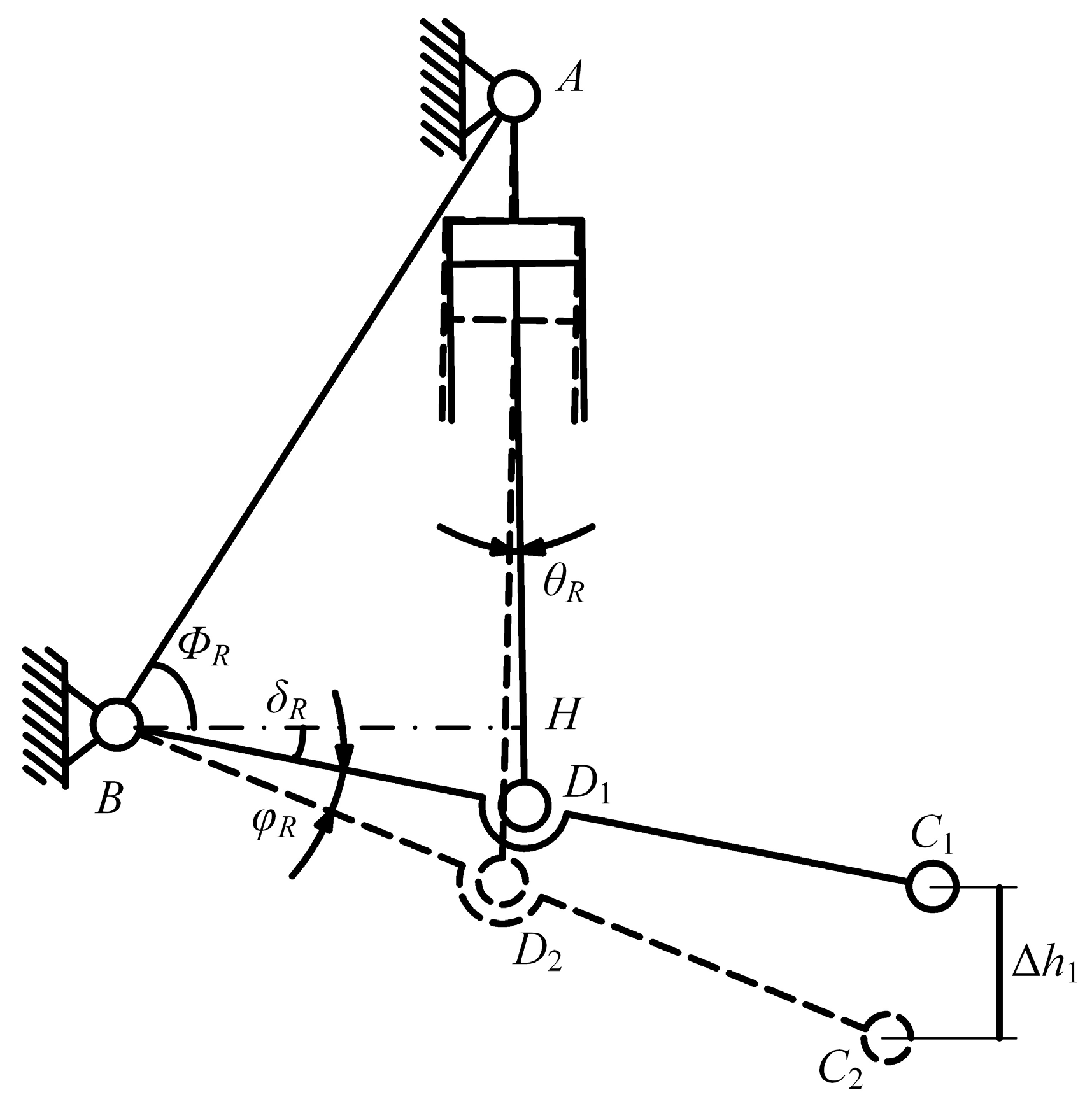
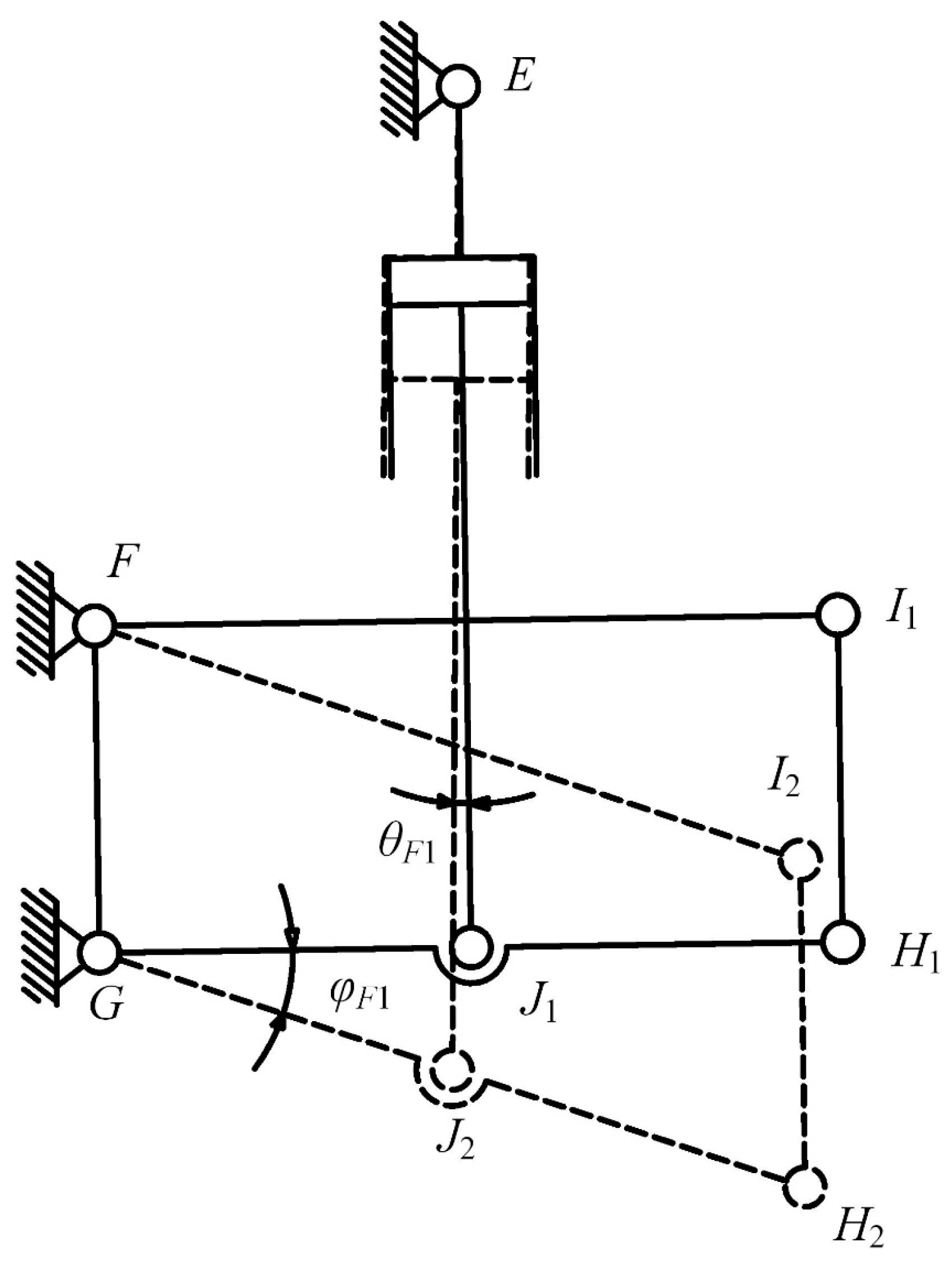
Appendix A. Derivation of the Suspension Structure Principle

Appendix A provides a detailed derivation of the structural mathematical model for the front and rear suspensions of the three-wheeled agricultural robot.
The mechanism principle of the rear wheel suspension is shown in Figure 3. Hinge points A and B are situated on the support seat of the rear wheel suspension. Line segment BC represents the single oblique arm, where segment BC1 represents the single oblique arm in its initial state and BC2 represents the single oblique arm during the leveling process. Line segment AD represents the actuator of the rear suspension, where segment AD1 represents the actuator in its initial state and AD2 represents the actuator during the leveling process. Point C is located on the floating bracket of the rear wheel. Assuming the chassis is horizontal in the initial state, then line segment AD1 is perpendicular to the horizontal plane. δR is the angle between line segment BC1 and the horizontal plane. θR is the angle between line segment AD2 and line segment AD1. φR is the angle between line segment BC2 and line segment BC1. ΔY represents the extension of line segment AD1 to AD2, that is, the elongation of the rear suspension actuator. The floating height, ∆h1, of the rear wheel during the leveling process is the vertical distance from point C1 to C2. Therefore, the floating height, ∆h1, of the rear wheel is:
Δ h 1 = B C 2 sin ( δ R + φ R ) B C 1 sin δ R
The floating height, ∆h1, and the extension of rear suspension actuator, ΔY, satisfy the following equation:
Δ Y = A B 2 + B D 2 2 2 A B · B D 2 · cos ( sin 1 ( Δ h 1 B C 2 + sin δ R ) δ R + cos 1 A B 2 + B D 1 2 A D 1 2 2 A B · B D 1 ) A D 1
Figure 5 shows the mechanism schematic diagram of the front wheel double-wishbone independent suspension. In Figure 5, hinge points E, F, and G are located on the support seat of the front suspension.
Line segment GH represents the lower wishbone, where segment GH1 represents the lower wishbone in its initial state and GH2 represents the lower wishbone during the leveling process. Line segment FI represents the upper wishbone, where segment FI1 represents the upper wishbone in its initial state and FI2 represents the upper wishbone during the leveling process. Line segment IH represents the floating bracket of the front wheel, where segment I1H1 represents the floating bracket in its initial state and I2H2 represents the floating bracket during the leveling process. Line segment EJ represents the actuator of the front suspension, where segment EJ1 represents the actuator of the front suspension in its initial state and segment EJ2 represents the actuator during the leveling process. Assuming the chassis is horizontal in the initial state, then line segment EJ1 is perpendicular to the horizontal plane.
Ignore the swing of the front suspension actuator to simplify theoretical calculations, as the swing angle θF1 is relatively small. When the swing angle of the upper and lower wishbones is φ F 1 , the floating height of the front wheel relative to the vehicle body is ∆h2. Correspondingly, the elongation of the suspension actuator is ∆X1, i.e., segment EJ1 extends to segment EJ2. As shown in Figure 5, ∆h2 represents the vertical height difference between point H1 and point H2. The calculation formula between ∆h2 and ∆X1 is expressed as:
Δ X 1 = Δ h 2 · G J 2 G H 2

Appendix B. Hydraulic Servo System Model of the Suspension Actuator

(1)
Valve flow equation
To simplify calculations, the following assumptions are made:
(a)
The supply pressure, Ps, is constant, and the return pressure, T, is zero;
(b)
Pressure losses in the pipes and valve chambers are neglected;
(c)
The flow coefficients of all throttling orifices of the servo valve are equal, denoted as Cd.
The valve flow equation can be expressed as:
Q 1 = C d ω X v 2 ρ [ S ( X v ) P s P 1 + S ( X v ) P 1 ] Q 2 = C d ω X v 2 ρ [ S ( X v ) P 2 + S ( X v ) P s P 2 ]
where Q1 represents the flow rate of the hydraulic valve into and out of the rodless chamber of the hydraulic cylinder, Q2 represents the flow rate of the hydraulic valve into and out of the rod chamber of the hydraulic cylinder, Xv represents the valve spool displacement, Ps represents the supply pressure, P1 represents the pressure in the rodless chamber, P2 represents the pressure in the rod chamber, ρ represents the fluid density, ω represents the valve port area gradient, and Cd represents the flow coefficient of the throttling orifice.
(2)
Hydraulic cylinder flow equation
To simplify calculations, the following assumptions are made:
(a)
Pressure losses and dynamic effects in the pipes are negligible;
(b)
The oil temperature and bulk modulus are constant;
(c)
Both internal and external leakage in the hydraulic cylinder are laminar.
The hydraulic cylinder flow equation is:
Q 1 = A 1 X ˙ 1 + C i p ( P 1 P 2 ) + [ C e p P 1 + V 1 + A 1 X 1 β e P ˙ 1 ] Q 2 = A 2 X ˙ 1 + C i p ( P 1 P 2 ) [ C e p P 2 + V 2 A 2 X 1 β e P ˙ 2 ]
where V1 represents the volume of the rodless chamber of the hydraulic cylinder, V2 represents the volume of the rod chamber of the hydraulic cylinder, A1 represents the effective piston area of the rodless chamber, A2 represents the effective piston area of the rod chamber, X1 represents the piston displacement of the hydraulic cylinder, βe represents the effective bulk modulus, Cip represents the internal leakage coefficient of the hydraulic cylinder, and Cep represents the external leakage coefficient of the hydraulic cylinder.
If the internal and external leakage and transient volume changes of the hydraulic cylinder are neglected, Equation (A6) can be simplified to:
Q 1 = A 1 X ˙ 1 + V 1 β e P ˙ 1 Q 2 = A 2 X ˙ 1 V 2 β e P ˙ 2
In Equation (A6), X 1 = Z 1 Z 2 . Substituting Equation (A6) into Equation (A4) yields the following equation.
P ˙ 1 = β e V 1 { C d ω X v 2 ρ [ S ( X v ) P s P 1 + S ( X v ) P 1 ] A 1 ( Z 1 · Z 2 · ) } P ˙ 2 = β e V 2 { C d ω X v 2 ρ [ S ( X v ) P 2 + S ( X v ) P s P 2 ] A 2 ( Z 1 · Z 2 · ) }
(3)
Hydraulic cylinder force balance equation
The force balance equation for the hydraulic cylinder is:
F 2 = A 1 P 1 A 2 P 2
Substituting Equation (A8) into Equation (6) yields the following equation.
Z ¨ 1 = A 1 P 1 A 2 P 2 + k s ( Z 2 Z 1 ) + c ( Z 2 Z 1 ) M 1 Z ¨ 2 = A 2 P 2 A 1 P 1 + k s ( Z 1 Z 2 ) + c ( Z 1 Z 2 ) + K ( w Z 2 ) M 2

References

  1. Dettù, F.; Corno, M.; D’Ambrosio, D.; Acquistapace, A.; Taroni, F.; Savaresi, S.M. Modeling, control design and experimental automatic calibration of a leveling system for combine harvesters. Control. Eng. Pract. 2023, 132, 105411. [Google Scholar] [CrossRef]
  2. Hu, J.; Pan, J.; Dai, B.; Chai, X.; Sun, Y.; Xu, L. Development of an attitude adjustment crawler chassis for combine harvester and Experiment of adaptive leveling system. Agronomy 2022, 12, 717. [Google Scholar] [CrossRef]
  3. Peng, H.; Ma, W.; Wang, Z.; Yuan, Z. Leveling Control of Hillside Tractor Body Based on Fuzzy Sliding Mode Variable Structure. Appl. Sci. 2023, 13, 6066. [Google Scholar] [CrossRef]
  4. Lü, X.; Liu, Z.; Lü, X.; Wang, X. Design and study on the leveling mechanism of the tractor body in hilly and mountainous areas. J. Eng. Des. Technol. 2024, 22, 679–689. [Google Scholar] [CrossRef]
  5. Jin, X.; Wang, J.; Yan, Z.; Xu, L.; Yin, G.; Chen, N. Robust vibration control for active suspension system of in-wheel-motor-driven electric vehicle via μ-synthesis methodology. J. Dyn. Syst. Meas. Control. 2022, 144, 051007. [Google Scholar] [CrossRef]
  6. Liu, S.; Zheng, T.; Zhao, D.; Hao, R.; Yang, M. Strongly perturbed sliding mode adaptive control of vehicle active suspension system considering actuator nonlinearity. Veh. Syst. Dyn. 2022, 60, 597–616. [Google Scholar] [CrossRef]
  7. Han, S.-Y.; Dong, J.-F.; Zhou, J.; Chen, Y.-H. Adaptive fuzzy PID control strategy for vehicle active suspension based on road evaluation. Electronics 2022, 11, 921. [Google Scholar] [CrossRef]
  8. Jayaraman, T.; Thangaraj, M. Standalone and interconnected analysis of an independent accumulator pressure compressibility hydro-pneumatic suspension for the Four-Axle Heavy Truck. Actuators 2023, 12, 347. [Google Scholar] [CrossRef]
  9. Chen, H.; Gong, M.; Zhao, D.; Zhu, J. Body attitude control strategy based on road level for heavy rescue vehicles. Proc. Inst. Mech. Eng. Part D J. Automob. Eng. 2021, 235, 1351–1363. [Google Scholar] [CrossRef]
  10. Liu, S.; Zhang, L.; Chen, M.; Yang, C.; Zhang, J.; Wang, J. Multiple Suspensions Coordinated Control for Corner Module Architecture Intelligent Electric Vehicles on Stepped Roads. IEEE Trans. Intell. Veh. 2024. [Google Scholar] [CrossRef]
  11. Zhang, N.; Yang, S.; Wu, G.; Ding, H.; Zhang, Z.; Guo, K. Fast distributed model predictive control method for active suspension systems. Sensors 2023, 23, 3357. [Google Scholar] [CrossRef] [PubMed]
  12. Hamza, A.; Ben Yahia, N. Artificial neural networks controller of active suspension for ambulance based on ISO standards. Proc. Inst. Mech. Eng. Part D J. Automob. Eng. 2023, 237, 34–47. [Google Scholar] [CrossRef]
  13. Fu, B.; Liu, B.; Di Gialleonardo, E.; Bruni, S. Semi-active control of primary suspensions to improve ride quality in a high-speed railway vehicle. Veh. Syst. Dyn. 2023, 61, 2664–2688. [Google Scholar] [CrossRef]
  14. Li, J.; Wang, J.; Chen, Y.; Si, E. Optimization of Suspension Active Control System Based on Improved Genetic Algorithm. In Proceedings of the 2023 7th International Conference on Electrical, Mechanical and Computer Engineering (ICEMCE), Xi’an, China, 25–27 October 2024; pp. 737–740. [Google Scholar]
  15. Jin, X.; Wang, J.; He, X.; Yan, Z.; Xu, L.; Wei, C.; Yin, G. Improving vibration performance of electric vehicles based on in-wheel motor-active suspension system via robust finite frequency control. IEEE Trans. Intell. Transp. Syst. 2023, 24, 1631–1643. [Google Scholar] [CrossRef]
  16. Ding, R.; Wang, R.; Meng, X.; Chen, L. Research on time-delay-dependent H∞/H2 optimal control of magnetorheological semi-active suspension with response delay. J. Vib. Control. 2023, 29, 1447–1458. [Google Scholar] [CrossRef]
  17. Maciejewski, I.; Blazejewski, A.; Pecolt, S.; Krzyzynski, T. A sliding mode control strategy for active horizontal seat suspension under realistic input vibration. J. Vib. Control. 2023, 29, 2539–2551. [Google Scholar] [CrossRef]
  18. Chen, G.; Jiang, Y.; Tang, Y.; Xu, X. Revised adaptive active disturbance rejection sliding mode control strategy for vertical stability of active hydro-pneumatic suspension. ISA Trans. 2023, 132, 490–507. [Google Scholar] [CrossRef] [PubMed]
  19. Nguyen, T.A. A novel approach with a fuzzy sliding mode proportional integral control algorithm tuned by fuzzy method (FSMPIF). Sci. Rep. 2023, 13, 7327. [Google Scholar] [CrossRef] [PubMed]
  20. Wu, L.; Zhao, D.; Zhao, X.; Qin, Y. Nonlinear adaptive back-stepping optimization control of the hydraulic active suspension actuator. Processes 2023, 11, 2020. [Google Scholar] [CrossRef]
  21. Nguyen, H.L.T. Lyapunov-based Design of a Model Reference Adaptive Control for Half-Car Active Suspension Systems. Meas. Control. Autom. 2024, 5, 22–29. [Google Scholar]
Figure 1. Three-dimensional structural diagram of the three-wheeled chassis.
Agronomy 14 01765 g001
Figure 2. Structural diagram of the rear wheel suspension.
Agronomy 14 01765 g002
Figure 3. Mechanism schematic diagram of the rear wheel suspension.
Agronomy 14 01765 g003
Figure 4. Structural diagram of the double-wishbone independent suspension used in the front wheels.
Agronomy 14 01765 g004
Figure 5. Mechanism schematic diagram of the front wheel double-wishbone independent suspension.
Agronomy 14 01765 g005
Figure 6. Force analysis model of the three-wheeled chassis.
Agronomy 14 01765 g006
Figure 7. Single-wheel suspension model.
Agronomy 14 01765 g007
Figure 8. Principle of the hydraulic actuator system for active suspension.
Agronomy 14 01765 g008
Figure 9. Logic diagram of the leveling control strategy.
Agronomy 14 01765 g009
Figure 10. Schematic diagram of the reference coordinate system for the three-wheeled chassis.
Agronomy 14 01765 g010
Figure 11. Logic flowchart of leveling control for the first category of chassis attitude (α = 0 or β = 0).
Agronomy 14 01765 g011
Figure 12. Control logic flowchart for leveling chassis attitudes in categories 2 to 5.
Agronomy 14 01765 g012
Figure 13. The three forms included in the second category of chassis attitudes (α > 0, β > 0). (a) Item 5; (b) Item 14; (c) Item 5.
Agronomy 14 01765 g013aAgronomy 14 01765 g013b
Figure 14. The structural principle of the composite controller.
Agronomy 14 01765 g014
Figure 15. Flowchart of the improved adaptive genetic algorithm.
Agronomy 14 01765 g015
Figure 16. Structural schematic diagram of the simulation model.
Agronomy 14 01765 g016
Figure 17. The simulation comparison curves of chassis attitude under convex road conditions. (a) Vehicle body centroid vertical displacement; (b) Vehicle body centroid vertical acceleration; (c) Roll angle; (d) Rolling angular acceleration; (e) Pitch angle; (f) Pitching angular acceleration.
Agronomy 14 01765 g017aAgronomy 14 01765 g017b
Figure 18. Three-wheeled agricultural robot prototype.
Agronomy 14 01765 g018
Figure 19. Arched one-sided bridge for testing.
Agronomy 14 01765 g019
Figure 20. Comparison of vehicle body attitude parameters on a convex road. (a) Vehicle body centroid vertical displacement; (b) Vehicle body centroid vertical acceleration; (c) Roll angle; (d) Rolling angular acceleration; (e) Pitch angle; (f) Pitching angular acceleration.
Agronomy 14 01765 g020aAgronomy 14 01765 g020b
Table 1. Notation.
Table 1. Notation.
SymbolDescription
ZbVehicle body centroid vertical displacement
αRoll angle of the three-wheeled agricultural robot
βPitch angle of the three-wheeled agricultural robot
ZA1Sprung mass displacement at the left front wheel
ZB1Sprung mass displacement at the right front wheel
ZC1Sprung mass displacement at the rear wheel
ZA2Wheel displacement of the left front wheel
ZB2Wheel displacement of the right front wheel
ZC2Wheel displacement of the rear wheel
wARoad excitation of the left front wheel
wBRoad excitation of the right front wheel
wCRoad excitation of the rear wheel
FA1Force of the left front wheel suspension on the chassis
FB1Force of the right front wheel suspension on the chassis
FC1Force of the rear wheel suspension on the chassis
FA2Controllable forces provided by the left front wheel suspension hydraulic actuators
FB2Controllable forces provided by the right front wheel suspension hydraulic actuators
FC2Controllable forces provided by the rear wheel suspension hydraulic actuators
cALeft front wheel suspension damping coefficients
cBRight front wheel suspension damping coefficients
cCRear wheel suspension damping coefficients
ksALeft front wheel suspension spring stiffness
ksBRight front wheel suspension spring stiffness
ksCRear wheel suspension spring stiffness
ktALeft front wheel tire stiffness
ktBRight front wheel tire stiffness
ktCRear wheel tire stiffness
MsSprung mass of the three-wheeled chassis
MwUnsprung mass of the three-wheeled chassis
MA1Sprung mass at the left front wheel
MB1Sprung mass at the right front wheel
MC1Sprung mass at the rear wheel
MA2Unsprung mass at the left front wheel
MB2Unsprung mass at the right front wheel
MC2Unsprung mass at the rear wheel
lfDistance between the two front wheel suspensions
lbDistance between the center of the two front wheel suspensions and the rear wheel suspension
lbfDistance between the vehicle body centroid and the center of the two front wheel suspensions
lbrDistance between the vehicle body centroid and the rear wheel suspension
IxPitch moment of inertia
IyRoll moment of inertia
MxPitch moment of the vehicle body
MyRoll moment of the vehicle body
XvValve spool displacement
PsSupply pressure
P1Pressure in the rodless chamber
P2Pressure in the rod chamber
ρFluid density
ωValve port area gradient
CdFlow coefficient of the throttling orifice
V1Volume of the rodless chamber of the hydraulic cylinder
V2Volume of the rod chamber of the hydraulic cylinder
A1Effective piston area of the rodless chamber
A2Effective piston area of the rod chamber
βeEffective bulk modulus
Table 2. The 19 attitudes of the three-wheeled chassis.
Item∆A∆B∆CαβChassis Attitude Classification Based on Angles α and β
100000α = 0, β = 0
200−10+α = 0, β > 0
30010α = 0, β < 0
4−100α < 0, β < 0
5100++α > 0, β > 0
60−10+α > 0, β < 0
7010+α < 0, β > 0
8−1−100α = 0, β < 0
91100+α = 0, β > 0
101−10+0α > 0, β = 0
11−1100α < 0, β = 0
12−10−1+α < 0, β > 0
13−101α < 0, β < 0
1410−1++α > 0, β > 0
15101+α > 0, β < 0
160−1−1++α > 0, β > 0
170−11+α > 0, β < 0
1801−1+α < 0, β > 0
19011α < 0, β < 0
Table 3. The main parameters of the simulation model.
VariablesValuesUnitsVariablesValuesUnitsVariablesValuesUnits
Ms1250kgMw400kg V 1 0.00098m3
ks20,000N/mc1000N·s·m⁻¹ V 2 0.00035m3
kt2 × 105N/mh0.1m β e 7 × 10⁸Pa
P s 1.6 × 10⁷Pa C d 0.6L2m
Ix525.5kg·m2Iy625.5kg·m2 ρ 900kg/m3
A 1 0.00196m2Lb1.84mlbf0.55m
A 2 0.0007m2Lf1.62mlbr1.29m
v 1m/s ω 0.0015m
Table 4. The peak values of chassis attitude parameters for the three leveling methods.
Leveling MethodVertical Displacement (m)Roll Angle (rad)Pitch Angle (rad)
Passive suspension0.0520.0320.028
PID 0.0410.0250.022
ADLCCS-SLM0.0290.0180.016
Table 5. The peak values of chassis attitude parameters in the test.
Leveling MethodVertical Displacement (m)Roll Angle (rad)Pitch Angle (rad)
PID0.0350.0220.018
ADLCCS-SLM0.0200.0150.012
Disclaimer/Publisher’s Note: The statements, opinions and data contained in all publications are solely those of the individual author(s) and contributor(s) and not of MDPI and/or the editor(s). MDPI and/or the editor(s) disclaim responsibility for any injury to people or property resulting from any ideas, methods, instructions or products referred to in the content.

