Abstract
The growth status of winter wheat seedlings during the greening period is called the seedling situation. Timely and accurate determinations of the seedling situation type are important for subsequent field management measures and yield estimation. To solve the problems of low-efficiency artificial classification, subjective doping, inaccurate classification, and overfitting in transfer learning in classifying the seedling condition of winter wheat seedlings during the greening period, we propose an improved ConvNeXt winter wheat seedling status classification and identification network based on the pre-training–fine-tuning model addressing over-fitting in transfer learning. Based on ConvNeXt, a SETFL-ConvNeXt network (Squeeze and Excitation attention-tanh ConvNeXt using focal loss), a winter wheat seedling identification and grading network was designed by adding an improved SET attention module (Squeeze and Excitation attention-tanh) and replacing the Focal Loss function. The accuracy of the SETFL-ConvNeXt reached 96.68%. Compared with the classic ConvNeXt model, the accuracy of the Strong class, First class, and Third class increased by 1.188%, 2.199%, and 0.132%, respectively. With the model, we also compared the effects of different optimization strategies, five pre-training-fine-tuning models, and the degree of change in the pre-trained model. The accuracy of the fine-tuning models trained in the remaining layers increased by 0.19–6.19% using the last three frozen blocks, and the accuracy of the pre-trained model increased by 3.1–8.56% with the least degree of change method compared with the other methods. The SETFL-ConvNeXt network proposed in this study has high accuracy and can effectively address overfitting, providing theoretical and technical support for classifying winter wheat seedlings during the greening period. It also provides solutions and ideas for researchers who encounter overfitting.
1. Introduction
Winter wheat is one of the most important grain crops in China, with an annual output of over 10,000 tons, making China the world’s largest wheat producer. In total, 95% of wheat is sown as winter wheat in autumn, while the rest is sown as spring wheat in the spring. Its yield and quality directly affect China’s food security [1]. The greening period is one of the most important stages of winter wheat growth and a crucial reflection of wheat seedling quality in agricultural production. The greening period is when the temperature rises in spring and plants begin to grow. The greening period occurs when 50% of the plants grow new leaves, the leaf sheaths extend 1–2 cm, and the leaf color changes from dark green to green, usually from late February to early March [2]. Different types of winter wheat seedlings correspond to different predicted yields and require corresponding field management techniques. Therefore, accurately classifying and identifying winter wheat seedling status is important for scientific agricultural production management [3,4].
Greening seedlings are traditionally detected through manual observation and empirical judgment, leading to problems such as strong subjectivity, large workload, and significant time consumption. This method cannot meet the requirements of efficiency, accuracy, and real-time processing. In addition to manual detection, image-processing technology is used in research, and machine learning researchers have manually designed feature extraction algorithms [5,6]. Peng Fang et al. [7] used 10-m-resolution images from the Sentinel-2 satellite combined with machine learning algorithms for large-scale winter wheat area recognition and mapping. Their study compared the classification performance and mechanism of three machine learning algorithms: support vector machine (SVM), random forest (RF), and classification regression tree (CART). The results showed that SVM performed the best in winter wheat recognition, with an overall accuracy of 0.94. Yuan Fang et al. [8] used laser radar to evaluate the tiller number of wheat in the field. They first used the adaptive hierarchical algorithm (AL) for clustering segmentation and then the hierarchical clustering algorithm (HC) for tiller detection between clusters. This algorithm estimated the tiller number of wheat, and the regression coefficient (R2) values were 0.61, 0.56, and 0.65. Lukas Roth et al. [5] used unmanned aerial vehicles (UAVs) to obtain multi-view images of quantified wheat leaf area changes by repeatedly flying over a breeding nursery with early single-row wheat plots. They used support vector machines to predict stem elongation and watershed algorithms and growth models to predict the seedling rate and tiller number. The results showed that the emergence rate R2 was 0.52, the tiller number R2 was 0.86, and the stem elongation R2 was 0.77. Related research has combined image-processing technology by manually designing feature extraction algorithms, but the effectiveness is extremely dependent on the researcher’s experience level; the transferability is low, with low accuracy. Moreover, some studies require specialized spectral or specialized equipment in specific fields.
With the rapid development of artificial intelligence, applying deep learning to image recognition has provided new ideas and methods for identifying and grading winter wheat seedlings during the greening period. Deep learning technology has a powerful advantage in its automatic learning features, and it has achieved significant results in fields such as image recognition, object detection, and image segmentation [9,10,11,12,13].
With the vigorous development of deep learning research, models are moving toward deeper levels and larger parameter quantities, and the requirements for datasets and training costs are increasing. This phenomenon is more prominent in large models. In the agricultural field, high-quality public datasets are relatively scarce. However, transfer learning has greatly improved this situation. The concept of transfer learning originates in machine learning. In a broad sense, transfer learning is a machine learning method that applies existing knowledge to solve different but related domain problems. Transfer learning is widely used in deep learning research owing to its powerful learning ability and limited training time [14,15,16]. A transfer learning paradigm based on pre-training–fine-tuning in deep learning is widely used by researchers [17]. ShengJie Teng et al. [18] used ConvNeXt to detect the substitution rate of steel sand by adding SE attention(Squeeze and Excitation attention) to the ConvNeXt Block. After the weights were transferred from one mixed sand group to three steel sand groups, the accuracy rate reached 92.64%, 4.65% higher than without transfer learning. Xiaoqi Wang et al. [19] used ConvNeXt to classify and recognize seven rice diseases, adding ECA (Efficient Channel Attention) between the convolution layer and the global average pool layer, with the frozen convolution layer only training itself. To avoid overfitting, the model parameters were divided into two parts: weights and biases. The attenuation operation was only used for weights, with an accuracy of 94.82%. Tongkai Li et al. [20] used transfer learning to grade the quality of Oudemansiella raphanipes; they froze the pre-trained model, trained the head model and FC layer, and used various optimization methods to improve model performance and avoid overfitting. The accuracy reached 98.75%, and the detection speed for one image was 22.5 ms. Although the above studies have effectively improved this model’s performance, they did not use the pre-training–fine-tuning method to effectively address overfitting; thus, the model only performed well when the dataset quality was good and the categories were relatively balanced.
ConvNeXtV2 is an optimized model based on Convnet. It is created by co-designing a fully convolutional masked autoencoder (FCMAE) and using global response normalization (GRN). Compared with ConvNeXt, the model is more complicated. ConvNeXt’s design is relatively simple and clear, which makes it easier to understand, de-bug and optimize. ConvNeXt provides a strong foundation for researchers and developers, without having to invest too much energy in complex self-monitoring training strategies. Although ConvNeXtV2 has improved its performance by introducing new technologies, ConvNeXt still has advantages in computing efficiency, simple architecture and mature stability.
There is little research on applying deep learning to winter wheat seedling status during the greening period. Although these studies have improved the recognition effect of crops to a certain extent, they often perform poorly in situations where the dataset samples are insufficient and the categories are not balanced. In the context of ensuring improved recognition accuracy, the requirements for computing resources are relatively high. This study aims to reduce labor costs, improve the accuracy and efficiency of detection, save model training costs, and better the complete identification and grading of winter wheat seedlings during the greening period.
Thus, to solve the problem of uneven recognition accuracy caused by uneven wheat seedling sample data classification, we improved the ConvNext network by changing the cross-entropy loss to focal loss and adding an improved SE attention module (SET) to reduce model overfitting and help the model better utilize image feature information. From the perspective of low recognition accuracy and saving computational resources, we compared the impact of data augmentation and transfer learning optimization methods on model performance. When using transfer learning to fine-tune a model, it is necessary to control overfitting. Using pre-training–fine-tuning techniques in transfer learning, we validated the impact of five fine-tuning methods on the network model, as well as the effect of different embedding attention methods on model performance.
2. Materials and Methods
2.1. Datasets
Image data for winter wheat seedlings during the greening period were acquired in March 2023 and March 2024. Over 2000 winter wheat plants were surveyed and harvested in Shengli Village, Pingdu City, Shandong Province, and Xizhai Village, Pingdu City, Shandong Province. Considering the practicality of the model under real-world conditions, no specialized shooting system is set up, only a smartphone needs to be used for shooting. Considering the distance of winter wheat in the image, both too bright and too dark can affect the model. By capturing images of winter wheat during the greening period at different orientations and distances (20 cm–50 cm) under daily brightness conditions, and the final dataset contained 2831 images. Of these, there were 689 Strong-class, 605 First-class, 1048 Second-class, and 489 Third-class images, and all were annotated. Unbalanced datasets negatively impact models, as they focus too much on the feature information in multi-class samples and ignore that of classes with fewer samples. Some scholars have solved this problem by oversampling or undersampling their datasets [21], but these optimization strategies are relatively complex and ultimately have unstable performance. Therefore, this study addresses this issue by replacing the focal loss function.
Detecting winter wheat seedlings focuses on several growth parameters, including the number of tillers per plant, the total tillers, secondary roots, and the leaf age of the main stem. We referred to the local standard in Shandong Province to define the greening period for winter wheat (DB 37/7T 4366-2021); that is, the date when the average temperature in spring stabilizes above 3 °C, the wheat seedlings resume growth, the leaves turn bright green, and the new leaves elongate by 1.5 cm–2 cm. We classify winter wheat seedlings into four types: Strong class, First class, Second class, and Third class.
While we drew on the local standard, we also made changes based on actual conditions, mainly focusing on the individual growth parameters of winter wheat. The five-point sampling method was used for field sampling plots with uniform growth, with 10 samples taken from each point to represent the growth of winter wheat seedlings on a mu of land. The specific classification criteria are as follows: The Strong class has more than 7 tillers per plant, the growth appearance is characterized by slender leaves, there are many albeit weak tillers, and there are more than 7 secondary roots per plant. The First-class has 5–6 tillers per plant, with green leaves and many large tillers, and there are 5–7 secondary roots on a single plant. The Second class has 3–4 tillers per plant, the growth appearance is green, and there are 3–4 secondary roots on a single plant. The Third class has 1–2 tillers per plant, with a growth appearance of light green leaves, small and weak tillers, and less than 3 secondary roots per plant.
We preprocessed the collected images, adjusted their sizes to 224 × 224, and performed data augmentation. We included 9 image transformation methods, including horizontal flipping, left and right rotation, narrowing, enlargement, random color changes, random occlusion, and Gaussian blur, as shown in Figure 1.
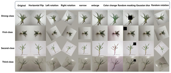
Figure 1.
Wheat dataset.
2.2. Transfer Learning and Pre-Training–Fine-Tuning
Pre-training–fine-tuning is an important technique in transfer learning. Pre-training refers to obtaining a pre-trained model by learning the basic features of images based on a large dataset. Fine-tuning involves making the pre-trained model more suitable for the new task. Usually, pre-trained models are not fully applicable to the new related task. By further learning and adjusting the parameters of the pre-trained model using the new task’s dataset, a target model suitable for the new task can be obtained. This process is called pre-training–fine-tuning [22,23]. The types of fine-tuning include the following:
Fine-tuning all layers: All parameters of the entire pre-trained model are retrained.
Fine-tuning some layers: The parameters at the bottom layer of the model are frozen, and only the parameters of the last FC layer or the last few layers of the model are retrained. The parameters of the other layers are frozen and remain unchanged, as shown in Figure 2.
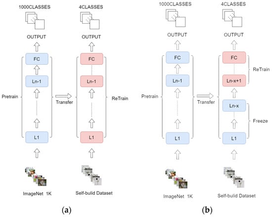
Figure 2.
Types of pre-training–fine-tuning. Fine-tuning all layers (a), Fine-tuning some layers (b).
The ConvNeXt pre-trained model used in this study is based on the original model under the Pytorch framework [24]. Its dataset is the publicly available ImageNet-1K [25]. To be more suitable for this task, the original 1000 classes in the FC were changed into 4 classes, an improved SET attention mechanism module was added, and the cross-entropy loss was changed to focal loss. Finally, a new SETFL-ConvNeXt network was obtained. The pre-training–fine-tuning model transfers convolution weights that have been trained for SETFL-ConvNeXt, and then, a self-built winter wheat dataset trains the model. Finally, the task of winter wheat seedling identification and grading during the greening period can be completed, as shown in Figure 3.
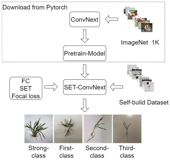
Figure 3.
Pre-training–fine-tuning flowchart.
3. Design of Model
3.1. Improved ConvNeXt Model
The ConvNeXt network model is a classic and popular convolutional model for image classification [26]. Our model is an improvement based on ConvNeXt Tiny. ConvNeXt draws inspiration from the structure of Swin Transformer [27], stacking ConvNeXt Blocks into a 3 × 3 × 9 × 3 pattern. We believe that the success of Swin Transformer relies not only on its innovative structural design but also on its various optimization methods. In this study, we used the idea of ConvNeXt for reference; pre-training–fine-tuning in transfer learning was used to enhance the performance indicators of our model for the task dataset and to speed up model convergence. The improved SE attention mechanism module was added to the model; that is, the tanh activation function was used to replace the original sigmoid activation function to reduce model overfitting, and the cross-entropy loss was changed to Focal loss to improve the impact of sample imbalance on the model, as shown in Figure 4. The model parameters before and after improvement are shown in Table 1.
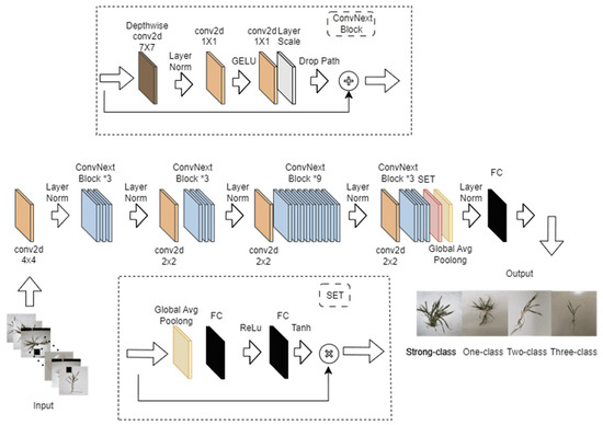
Figure 4.
Improved ConvNeXt structure.

Table 1.
Model structure parameter table.
3.2. Attention Mechanism Module
The SE attention module consists of the following two steps: [28].
- Squeeze: The input feature map is subjected to a global average pooling operation to obtain the global perception of each channel.
- Excitation: The compressed features are passed through a fully connected layer (usually consisting of two fully connected layers and an activation function) to generate weights for each channel; then, the weight coefficients are obtained through an activation function (usually sigmoid). These weight coefficients are multiplied element by element with the channels of the original input feature map, and the feature map is readjusted.
Based on the SE module, the tanh activation function is used instead of the sigmoid activation function to obtain the SET attention mechanism to suppress model overfitting and better transfer gradients during the training process, possibly improving the model’s overall performance.
3.3. Loss Function
In the Qingdao area of Shandong Province, the greening period for winter wheat is from late February to mid-March each year, making it difficult to collect wheat images. In addition, given the uneven distribution of wheat seedlings in the field, there is a significant imbalance in the distribution of seedling levels in the winter wheat dataset.
To address this issue, the focal loss function is used to optimize the model’s training process [29]. Focal loss is a loss function designed to solve class imbalance problems. It adjusts the weights of difficult and easy samples to make the model pay more attention to difficult-to-classify samples during training, thereby improving the overall classification performance. Specifically, focal loss introduces a moderating factor based on traditional cross-entropy loss, reducing the loss of simple samples and increasing the loss of difficult samples. This method can effectively alleviate model bias caused by imbalanced datasets and improve classification performance in imbalanced datasets
By applying the focal loss function, we hope to more accurately classify wheat images of different seedling levels, improve the model’s performance in practical applications, and provide more reliable data support for winter wheat growth monitoring.
Here, is the prediction confidence score of the model. The closer it is to 1, the more accurate the model classification is, and vice versa. balances the importance indicators of the positive and negative samples; is the focus on the parameters; and is the modulation coefficient. When a class of samples is misclassified and is very small, approaches 1, so the loss of difficult samples will not be affected; when approaches 1, approaches 0, and the weight of easy-to-classify samples decreases, making the model more focused on training difficult-to-classify samples.
4. Experimental Validation and Analysis of the Results
4.1. Configuration Environment
The experimental environment was the Windows 10 operating system; the CPU was an AMD EPYC 7402 24 Core Processor; the main frequency was 2.79 GHz; the Python 3.8.18 development environment was used; Pytorch 2.0.0 and CUDA12.2 were selected as the deep learning framework; an NVIDIA GeForce RTX 3090 was used for GPU operation acceleration; and the running memory of the GPU was 24 GB. The input image size was 224 pixels × 224 pixels; there were 50 training rounds; the batch size was 128; and the chosen optimizer was AdamW, using an exponential learning rate adjustment strategy with a parameter of 0.99.
4.2. Evaluation Indicators
Here, is the number of samples correctly predicted as positive, that is, the number of winter wheat seedling classes correctly classified and identified; is the number of samples correctly predicted as negative samples, that is, the number of winter wheat seedlings classified and identified as other classes; is the number of samples incorrectly predicted as positive, that is, the number of winter wheat seedling classes incorrectly classified and identified; is the number of samples incorrectly predicted as negative samples, that is, the number of winter wheat seedlings classified and identified as other classes. The F1 value is the harmonic mean of precision and recall. Accuracy represents the accuracy of the model.
4.3. The Impact of Different Learning Methods and Data Augmentation on Models
We compared the dataset before and after data augmentation using transfer learning training methods. The pre-training–fine-tuning mode in transfer learning uses full fine-tuning in the following ways:
① Using transfer learning without data augmentation;
② Using data augmentation without transfer learning;
③ Not using transfer learning or data augmentation;
④ Using transfer learning and data augmentation.
For models that only use data augmentation strategies without transfer learning, overfitting occurs after 20 epochs (Figure 5). The loss value of the model decreases and then increases, while the accuracy is basically unchanged. The enhanced data do not improve the generalization ability of the model but do introduce noise, resulting in the model learning too many noisy features. Both models using transfer learning strategies reached stability after five epochs, indicating that the convergence speed of the models was faster when using transfer learning. Thus, the accuracy of the models increased by 10.82% compared with the cases using and not using data augmentation. When neither optimization strategy was used, the model’s loss curve converges at 25 epochs, and the accuracy can only reach 75.65%. Using transfer learning can not only accelerate the convergence speed of the model but also utilize the rich underlying features of large data to improve its generalization ability and overall performance.
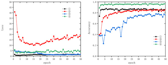
Figure 5.
Loss and accuracy of transfer learning and data augmentation.
The two models that only use one of the two optimization strategies have an impressive training set accuracy of around 99% (Table 2), but their test sets are only around 85%, indicating that they have learned a large number of useless features and ignored general and generalizable features, leading to overfitting.
Table 2.
Loss and accuracy of transfer learning and data augmentation.
4.4. The Impact of Pre-Training–Fine-Tuning Methods on the Model
In many studies, researchers default to using partial fine-tuning when using transfer learning techniques, freezing the previous network results and only training the last few layers of the network, except for the convolutional layer or the last FC layer. Some scholars choose different fine-tuning methods based on the degree of difference between the large dataset learned by the pre-trained model and the task dataset [30,31]. There is currently no definitive conclusion on the impact of different fine-tuning methods on this model, but one thing is certain: training with a larger sample size dataset can achieve better results. However, this also increases costs and training times.
This experimental design includes
Global fine-tuning (A);
Partial fine-tuning (B) to train only the last layer of the FC layer and the SET attention mechanism;
Partial fine-tuning (C) to train the last three layers of the ConvNeXt Block and the last layer of the FC layer and SET attention mechanism;
Partial fine-tuning (D) to freeze the first six layers of the ConvNeXt Block to train the remaining layers;
Partial fine-tuning (E) to freeze the first three layers of to ConvNeXt Block to train the remaining layers.
Figure 6 shows that the accuracy of the partially fine-tuned C model trained on the last three layers of the ConvNeXt Block, the last layer of the FC layer, and the SET attention mechanism reached 0.9668. Compared with the globally fine-tuned A model, the partially fine-tuned B model trained only on the last layer of the FC layer and the SET attention mechanism with the lowest accuracy, the partially fine-tuned D model trained on the remaining layers of the first six frozen ConvNeXt Blocks, and the partially fine-tuned E model trained on the remaining layers of the first three frozen ConvNeXt Blocks, the C model’s accuracy increased by 0.19%, 6.19%, 0.44%, and 0.75%, respectively.
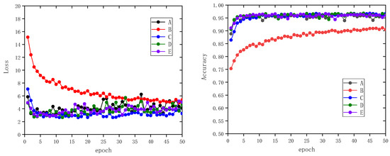
Figure 6.
Loss and accuracy of pre-training–fine-tuning methods in the test set.
The convergence speed shown in Figure 6 reveals that the B model exhibited a convergence trend after approximately 45 rounds. This indicates that the number of fine-tuning layers and fine-tuning strategies significantly impacts the convergence speed of the model. Because it only fine-tunes the last FC layer, the B model lacks adjustments for deeper features, resulting in a slower convergence speed and lower accuracy. The C model performs the best by fine-tuning multiple deep feature layers and attention mechanisms to better capture features and converge quickly.
The loss curve shows that the C model performs best with no significant oscillations or upward trends, indicating that the model maintains a stable learning process during training. By contrast, the curve oscillation of the A model is the most significant, possibly because global fine-tuning involves many parameter updates during the training process, making it difficult for the model to optimize smoothly. The curve of the B model is relatively smooth, but its learning effect is limited by the few fine-tuning layers. The D and E models also exhibit a certain degree of oscillation, but they are still relatively stable overall.
4.5. The Impact of Insertion Position on the Model
Attention mechanisms have attracted much attention, and the flexible use of plug-and-play attention mechanisms can greatly improve the performance indicators of a model. In a pre-training–fine-tuning paradigm transfer learning, adding an attention mechanism module suitable for the target task—in addition to changing the FC layer of the last layer of the pre-trained model according to the target task requirements and the appropriate method of embedding the attention mechanism module—has a significant impact on the model’s performance. In this section, we design an experiment to explore the impact of embedding the attention mechanism module on the model’s performance.
Model V is the original ConvNeXt model using global fine-tuning;
Model IV replaces ConvNeXt Block IV with a SET-ConvNeXt Block and freezes the rest of the layers, only training the SET-ConvNeXt Block and the FC layer;
Model III replaces ConvNeXt Block III and ConvNeXt Block IV with a SET-ConvNeXt Block and freezes the remaining layers, only training the SET-ConvNeXt Block and the FC layer;
Model II replaces ConvNeXt Block II, ConvNeXt Block III, and ConvNeXt Block IV with a SET-ConvNeXt Block and freezes the remaining layers, only training the SET-ConvNeXt Block and the FC layer;
Model I replaces ConvNeXt Block I, ConvNeXt Block II, ConvNeXt Block III, and ConvNeXt Block IV with a SET-ConvNeXt Block and freezes the remaining layers, only training the SET-ConvNeXt Block and the FC layer;
Model C puts the attention mechanism in Section 4.4, outside of the Block.
In this section, we take the common example of placing attention mechanisms in ConvNeXt Blocks, as shown in Figure 7, to compare and analyze the model with the C model in Section 4.4, placing attention outside of the ConvNeXt Blocks.
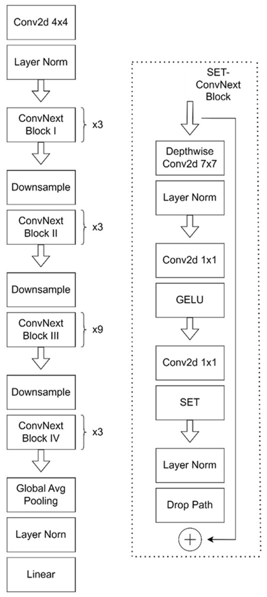
Figure 7.
SET insertion position.
As the attention mechanism is inserted, the degree of change in the pre-trained model increases for models IV, III, II, and I. Based on this loss, Figure 8 shows that three models (I, II, and III) exhibit overfitting where the loss values decrease and then increase. However, directly training the original ConvNeXt network (model V) using the fully fine-tuned method resulted in significant fluctuations in the loss curve, and the model learned too many redundant features. The IV loss value of the model with fewer structural changes first decreases and then reaches stability. As the original pre-trained model structure changes more, the model’s accuracy also decreases. The C model with the highest accuracy reaches 0.9668; the original network V accuracy is 0.9577; and the other four models are model IV at 0.9358, model III at 0.9224, model II at 0.8959, and model I at 0.8812. This indicates that changing the insertion attention mechanism has different effects on the feature extraction ability of the pre-trained model. The greater the damage to the feature extraction of the pre-trained model, the worse the performance. By contrast, the pre-trained model with the least changes in structure showed an accuracy improvement of 3.1–8.56% compared with the other methods, as well as an accuracy improvement of 0.91% compared with not changing the pre-trained model structure. Overfitting in the model also improved to some extent. Against the backdrop of the original ConvNeXt network having relatively high accuracy in this task, the pre-trained model with the least changes, structure C, improved accuracy by 0.91% compared with the original ConvNeXt model (V), and model overfitting improved to some extent. Through fine-tuning and improvement, the model better adapts to specific task requirements based on the target dataset. This means that the model learns more useful features rather than simply remembering noise or irrelevant patterns in the training data, thereby reducing overfitting. The weights in the pre-trained model are initially trained on large-scale datasets and may not directly adapt to the target task. During the fine-tuning process, the model learns a more suitable feature representation for the current task by further training on the target dataset, improving the model’s classification ability. Thus, the effectiveness of the optimization strategy has been verified. Optimization strategies include adjusting and changing the network structure, freezing some layer weights, and data augmentation. These operations help the model generalize better, avoiding overfitting while improving accuracy.
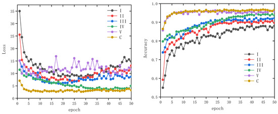
Figure 8.
Loss and accuracy of SET insertion position in the test.
4.6. Model Comparison
To verify the improved SETFL-ConvNeXt model’s performance, ablation experiments were carried out on the classic ConvNeXt network, ConvNeXt-FocalLoss, and SET-ConvNeXt-cross-entropy. At the same time, the proposed SETFL-ConvNeXt network model was compared with the classical networks in other image classification tasks [32,33,34,35]. Using data augmentation and transfer learning, the same super-parameter was set, and the results of the test set are shown in Table 2.
When compared with EfficientNet_v2s, MobileNet_V3s, ResNet18, and Vgg11, the accuracy of the classic ConvNeXt network was improved by 0.86%, 3.41%, 1.17%, and 1.52%, respectively (Table 3). The accuracy of the ConvNext_base model was 0.05% higher than that of ConvNext(ConvNext_tiny), but the model was not adopted because it is too large and consumes too many computing resources.
Table 3.
Average F1 and accuracy.
Compared with the MobileNet_V3s model with the lowest accuracy, the accuracy of the SETFL-ConvNeXt model improved by 4.27%. Compared with ConvNeXt_base, EfficientNet_v2s, ResNet18, and Vgg11, it increased by 0.86%, 1.72%, 2.03%, and 2.38%, respectively. The performance of SETFL-ConvNeXt is better than that of traditional networks.
Compared with the classical ConvNeXt network, the SET-ConvNeX-cross-entropy network, and the ConvNeXt-FL network, the accuracy of the SETFL-ConvNeXt model improved by 0.91%, 0.14%, and 0.21%, respectively. These improvements are mainly due to two key improvement measures: First, introducing the SET module enables the model to automatically learn more appropriate classification weights and focus on the feature information with high values. This ability significantly improves the discriminant ability of the model when dealing with complex scenes. Second, by using the focal loss function, the model can pay more attention to a small number of samples and difficult samples, effectively reducing the adverse effects of these samples on the overall model performance. These two improvement measures work together to further improve the model’s accuracy.
The analysis of the confusion matrix shows that the characteristics of the First-class seedlings are more similar to those of the Strong-class seedlings in the distribution of the four types (Figure 9). The data volume of one seedling type is smaller among the four types, and its classification accuracy is the lowest. In the classic ConvNeXt model, the accuracy for First-class seedlings is only 90.736%. To resolve this issue, we optimized for imbalanced data. By using the focal loss function, the ConvNeXt-FL model could improve its accuracy for First-class seedlings to 94.070%, 3.334% higher than the classical ConvNeXt model. In addition, the F1 values of the ConvNeXt-FL model increased by 0.8%, 1.0%, 0.6%, and 0.7% for the four seedling conditions, and the overall F1 value increased by 0.8%. These results indicate that focal loss performs well in dealing with imbalanced datasets and helps improve the model’s classification performance for minority classes. Meanwhile, after incorporating the SET attention mechanism, the SET-ConvNeXt model improved classification accuracy by 1.188%, 2.199%, and 0.132% compared with the classical ConvNeXt model for Strong-class, First-class, and Third-class seedlings. The accuracy for Second-class seedlings only slightly decreased by 0.034%. These results further demonstrate that introducing the SET module effectively enhances the feature extraction capability of the model and improves its generalization performance; in situations where features are similar or data are scarce, the model can still maintain good performance. The final SETFL-ConvNeXt network comprehensively utilizes the above advantages, and the accuracy for the four seedling types increased by 0.828%, 2.521%, 0.263%, and 0.401%.
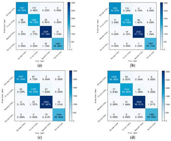
Figure 9.
Confusion matrix of the ablation experiment. ConvNeXt (a), SET-ConvNeXt-CE (b), ConvNeXt-FL (c), SETFL-ConvNeXt (d).
5. Discussion
Classifying winter wheat seedlings during the greening period still relies on manual labor in many places, with inconsistent standards and subjective assumptions. Using spectroscopic equipment or other fixed facilities to capture canopy images can be costly. This article starts from reality and considers the model’s practicality in real conditions. There is no need to set up a specialized shooting system, only to use a smartphone to collect winter wheat images. This method aims to assist government officials, researchers, and agricultural practitioners in classifying winter wheat seedlings during the greening period more conveniently and quickly, understanding the growth status of winter wheat, and providing a reference for subsequent field management. It also provides a solution and approach for researchers to address overfitting.
We found that when pre-trained models are used in transfer learning, targeted improvements are needed based on the characteristics and differences in downstream tasks. In classifying winter wheat seedlings during the greening period, owing to the small First-class seedling sample size in the dataset and its similarity to the characteristics of Strong-class seedlings, the expected model performance could not be achieved. Therefore, it is necessary to improve the model’s attention to important features. In addition, it is necessary to focus on addressing the common overfitting phenomenon in the transfer learning process. The research in this article yielded the following key results:
- Combining transfer learning and data augmentation can effectively improve the performance of models on training and testing sets and is thus an important means of enhancing model performance. When only data augmentation was performed on the dataset, the model exhibited overfitting. However, by using both optimization strategies simultaneously, the accuracy was improved by 20.84%. The model’s performance under different strategies indicates that reasonably selecting and combining training strategies can significantly enhance a model’s generalization ability and avoid overfitting.
- In the transfer learning process, it is important to choose appropriate fine-tuning strategies based on the characteristics of downstream tasks. Compared with the other four fine-tuning strategies, training the last three block layers, FC layer, and the partial fine-tuning of the SET attention mechanism improved the model’s accuracy by 0.19–6.19%.
- When using attention mechanisms to improve model performance, appropriate embedding methods should be selected based on the degree of change in the pre-trained model’s structure. As the degree of change decreases, the model’s accuracy increases, and overfitting is improved. For classifying winter wheat greening seedlings, selecting the method with the least degree of damage can achieve 0.9668 accuracy. Compared with other methods, the accuracy increased by 3.1–8.56%, and compared with not changing the structure of the pre-trained model, the accuracy increased by 0.91%.
- The SETFL-ConvNeXt model not only successfully improved the overall classification accuracy of the model to 0.9668 by introducing the focal loss and SET modules but also significantly improved the model’s performance in dealing with data imbalance and similar features. For classifying First-class seeding, the accuracy rate significantly improved by 2.521%, showing the effectiveness and practicability of these improvement measures.
Choosing appropriate optimization strategies and utilizing both transfer learning and image enhancement can enhance the practicality of a model. When selecting a plug-and-play attention module based on the characteristics of downstream tasks, ap-propriate fine-tuning methods should be combined with the model to complete down-stream target tasks. It is necessary to make appropriate adjustments to any overfitting to ensure the model’s generalization ability.
Compared with previous studies [11,18,19,20], our method provides a more robust framework for handling agricultural tasks that require precise classification. Although the above model has been successfully applied to the target task, our SETFL-ConvNeXt model has the highest accuracy in winter wheat classification. When using fine-tuning, only changing the FC layer or completely fine-tuning [18,20] may result in insufficient model performance or overfitting. Training the FC layer separately may result in the loss of complex features during the transmission from the convolutional layer to the FC layer, affecting the classification ability of the model. Global fine-tuning may also disrupt the common features learned by early layers in the pre trained model, leading to a decrease in model accuracy or overfitting. This indicates that the architecture and fine-tuning strategies of the model play a crucial role in its success.
Future work can focus on expanding the dataset to include more diverse types and regions, which may improve the model’s generalization ability in different agricultural contexts. In addition, attention should be paid to how to maintain the efficiency and accuracy of the model in various complex environments, in order to meet the needs of practical applications. After appropriate adjustments, the SETFL-ConvNeXt model not only has the potential to improve the classification of winter wheat seedlings, but also to extend its application to other crops and agricultural tasks, providing smarter and more refined technical support for agricultural production.
6. Conclusions
Our research shows that the combination of transfer learning and data augmentation significantly improves the model’s generalization ability and overall performance. Specifically, when applying these two strategies, the accuracy of the model increased by 20.84%. In transfer learning, selecting appropriate fine-tuning strategies for downstream tasks and combining them with attention mechanisms are key to improving model performance. By fine-tuning the last three layers and SET module of SETFL-ConvNeXt, the accuracy of the model has been significantly improved. The model has better adapted to the target task, learned more generalized features, and significantly improved overfitting. By using the embedding method with minimal structural changes, the model accuracy reached 96.68%. In addition, the use of SETFL-ConvNeXt model, especially the introduction of Focalloss and SET modules, effectively solved the challenges of data imbalance and feature similarity, and improved the classification accuracy of winter wheat in Frist-class by 2.521%.
Author Contributions
Conceptualization, C.L., Y.Y. and L.Z.; methodology, C.L.; software, C.L.; validation, Y.Y., S.W., and J.X.; formal analysis, C.L.; investigation, Y.Y., R.Q, S.W., and J.X.; resources, Y.Y. and L.Z.; data curation, C.L.; writing—original draft preparation, C.L. and R.Q.; writing—review and editing, C.L., R.Q. and J.Z.; visualization, R.Q.; supervision, L.Z.; project administration, C.L.; funding acquisition, Y.Y. and L.Z. All authors have read and agreed to the published version of the manuscript.
Funding
This study was funded by the National Natural Science Foundation of China (32071911), the National Key Research and Development Program (2023YFD2000404-1), and the Shandong Modern Agricultural Industry System Wheat Industry Innovation Team (SDAIT-01-13).
Data Availability Statement
The data are contained within the article.
Conflicts of Interest
The authors declare no conflicts of interest.
References
- He, D.; Fang, S.; Liang, H.; Wang, E.; Wu, D. Contrasting Yield Responses of Winter and Spring Wheat to Temperature Rise in China. Environ. Res. Lett. 2020, 15, 124038. [Google Scholar] [CrossRef]
- Girma, K.; Holtz, S.; Tubaña, B.; Solie, J.; Raun, W. Nitrogen Accumulation in Shoots as a Function of Growth Stage of Corn and Winter Wheat. J. Plant Nutr. 2010, 34, 165–182. [Google Scholar] [CrossRef]
- Qiong, W.; Cheng, W.; Jingjing, F.; Jianwei, J. Field Monitoring of Wheat Seedling Stage with Hyperspectral Imaging. Biol. Eng. 2016, 9. [Google Scholar]
- Liu, T.; Yang, T.; Li, C.; Li, R.; Wu, W.; Zhong, X.; Sun, C.; Guo, W. A Method to Calculate the Number of Wheat Seedlings in the 1st to the 3rd Leaf Growth Stages. Plant Methods 2018, 14, 101. [Google Scholar] [CrossRef]
- Roth, L.; Camenzind, M.; Aasen, H.; Kronenberg, L.; Barendregt, C.; Camp, K.-H.; Walter, A.; Kirchgessner, N.; Hund, A. Repeated Multiview Imaging for Estimating Seedling Tiller Counts of Wheat Genotypes Using Drones. Plant Phenomics 2020, 2020, 2020–3729715. [Google Scholar] [CrossRef] [PubMed]
- Liu, T.; Zhao, Y.; Wu, F.; Wang, J.; Chen, C.; Zhou, Y.; Ju, C.; Huo, Z.; Zhong, X.; Liu, S.; et al. The Estimation of Wheat Tiller Number Based on UAV Images and Gradual Change Features (GCFs). Precis. Agric. 2022, 24. [Google Scholar] [CrossRef]
- Fang, P.; Zhang, X.; Wei, P.; Wang, Y.; Zhang, H.; Liu, F.; Zhao, J. The Classification Performance and Mechanism of Machine Learning Algorithms in Winter Wheat Mapping Using Sentinel-2 10 m Resolution Imagery. Appl. Sci. 2020, 10, 5075. [Google Scholar] [CrossRef]
- Fang, Y.; Qiu, X.; Guo, T.; Wang, Y.; Cheng, T.; Zhu, Y.; Chen, Q.; Cao, W.; Yao, X.; Niu, Q.; et al. An Automatic Method for Counting Wheat Tiller Number in the Field with Terrestrial LiDAR. Plant Methods 2020, 16, 132. [Google Scholar] [CrossRef]
- Wang, H.; Shang, S.; Wang, D.; He, X.; Feng, K.; Zhu, H. Plant Disease Detection and Classification Method Based on the Optimized Lightweight YOLOv5 Model. Agriculture 2022, 12, 931. [Google Scholar] [CrossRef]
- Patricio, D.I.; Rieder, R. Computer Vision and Artificial Intelligence in Precision Agriculture for Grain Crops: A Systematic Review. Comput. Electron. Agric. 2018, 153, 69–81. [Google Scholar] [CrossRef]
- Li, D.; Zhai, M.; Piao, X.; Li, W.; Zhang, L. A Ginseng Appearance Quality Grading Method Based on an Improved ConvNeXt Model. Agronomy 2023, 13, 1770. [Google Scholar] [CrossRef]
- Kaya, A.; Keceli, A.S.; Catal, C.; Yalic, H.Y.; Temucin, H.; Tekinerdogan, B. Analysis of Transfer Learning for Deep Neural Network Based Plant Classification Models. Comput. Electron. Agric. 2019, 158, 20–29. [Google Scholar] [CrossRef]
- Lin, J.; Chen, X.; Cai, J.; Pan, R.; Cernava, T.; Migheli, Q.; Zhang, X.; Qin, Y. Looking from Shallow to Deep: Hierarchical Complementary Networks for Large Scale Pest Identification. Comput. Electron. Agric. 2023, 214, 108342. [Google Scholar] [CrossRef]
- Liu, B.; Cai, Y.; Guo, Y.; Chen, X. TransTailor: Pruning the Pre-Trained Model for Improved Transfer Learning. In Proceedings of the AAAI Conference on Artificial Intelligence, Virtual, 2–9 February 2021; Volume 35, pp. 8627–8634. [Google Scholar] [CrossRef]
- You, K.; Liu, Y.; Wang, J.; Long, M. LogME: Practical Assessment of Pre-Trained Models for Transfer Learning. In Proceedings of the 38th International Conference on Machine Learning, Online, 18–24 July 2021. [Google Scholar]
- Subramanian, M.; Shanmugavadivel, K.; Nandhini, P.S. On Fine-Tuning Deep Learning Models Using Transfer Learning and Hyper-Parameters Optimization for Disease Identification in Maize Leaves. Neural Comput. Appl. 2022, 34, 13951–13968. [Google Scholar] [CrossRef]
- Guo, Y.; Shi, H.; Kumar, A.; Grauman, K.; Rosing, T.; Feris, R. SpotTune: Transfer Learning through Adaptive Fine-Tuning. In Proceedings of the IEEE/CVF Conference on Computer Vision and Pattern Recognition, Long Beach, CA, USA, 15–20 June 2019. [Google Scholar]
- Teng, S.; Zhu, L.; Li, Y.; Wang, X.; Jin, Q. ConvNeXt Steel Slag Sand Substitution Rate Detection Method Incorporating Attention Mechanism. Sci. Rep. 2023, 13, 10593. [Google Scholar] [CrossRef] [PubMed]
- Wang, X.; Wang, Y.; Zhao, J.; Niu, J. ECA-ConvNeXt: A Rice Leaf Disease Identification Model Based on ConvNeXt. In Proceedings of the IEEE/CVF Conference on Computer Vision and Pattern Recognition, Vancouver, BC, Canada, 18–22 June 2023. [Google Scholar]
- Li, T.; Huang, H.; Peng, Y.; Zhou, H.; Hu, H.; Liu, M. Quality Grading Algorithm of Oudemansiella Raphanipes Based on Transfer Learning and MobileNetV2. Horticulturae 2022, 8, 1119. [Google Scholar] [CrossRef]
- More, A. Survey of Resampling Techniques for Improving Classification Performance in Unbalanced Datasets. arXiv 2016, arXiv:1608.06048. [Google Scholar]
- Iman, M.; Arabnia, H.R.; Rasheed, K. A Review of Deep Transfer Learning and Recent Advancements. Technologies 2023, 11, 40. [Google Scholar] [CrossRef]
- Basha, S.H.S.; Vinakota, S.K.; Pulabaigari, V.; Mukherjee, S.; Dubey, S.R. AutoTune: Automatically Tuning Convolutional Neural Networks for Improved Transfer Learning. Neural Netw. 2021, 133, 112–122. [Google Scholar] [CrossRef]
- Paszke, A.; Gross, S.; Massa, F.; Lerer, A.; Bradbury, J.; Chanan, G.; Killeen, T.; Lin, Z.; Gimelshein, N.; Antiga, L.; et al. PyTorch: An Imperative Style, High-Performance Deep Learning Library. Adv. Neural Inf. Process. Syst. 2019, 32. [Google Scholar]
- Ridnik, T.; Ben-Baruch, E.; Noy, A.; Zelnik-Manor, L. ImageNet-21K Pretraining for the Masses. arXiv 2021, arXiv:2104.10972. [Google Scholar]
- Liu, Z.; Mao, H.; Wu, C.-Y.; Feichtenhofer, C.; Darrell, T.; Xie, S. A ConvNet for the 2020s. In Proceedings of the 2022 IEEE/CVF Conference on Computer Vision and Pattern Recognition (CVPR), New Orleans, LA, USA, 18–24 June 2022; IEEE: New Orleans, LA, USA, 2022; pp. 11966–11976. [Google Scholar]
- Liu, Z.; Lin, Y.; Cao, Y.; Hu, H.; Wei, Y.; Zhang, Z.; Lin, S.; Guo, B. Swin Transformer: Hierarchical Vision Transformer Using Shifted Windows. In Proceedings of the IEEE/CVF International Conference on Computer Vision, Montreal, QC, Canada, 10–17 October 2021. [Google Scholar]
- Hu, J.; Shen, L.; Sun, G. Squeeze-and-Excitation Networks. In Proceedings of the 2018 IEEE/CVF Conference on Computer Vision and Pattern Recognition, Salt Lake City, UT, USA, 18–23 June 2018; IEEE: Salt Lake City, UT, USA, 2018; pp. 7132–7141. [Google Scholar]
- Mukhoti, J.; Kulharia, V.; Sanyal, A.; Golodetz, S.; Torr, P.H.S.; Dokania, P.K. Calibrating Deep Neural Networks Using Focal Loss. Adv. Neural Inf. Process. Syst. 2020, 33, 15288–15299. [Google Scholar]
- Kandel, I.; Castelli, M. How Deeply to Fine-Tune a Convolutional Neural Network: A Case Study Using a Histopathology Dataset. Appl. Sci. 2020, 10, 3359. [Google Scholar] [CrossRef]
- Kumar, A.; Raghunathan, A.; Jones, R.; Ma, T.; Liang, P. Fine-Tuning Can Distort Pretrained Features and Underperform Out-of-Distribution. arXiv 2022, arXiv:2202.10054. [Google Scholar]
- Liu, S.; Deng, W. Very Deep Convolutional Neural Network Based Image Classification Using Small Training Sample Size. In Proceedings of the 2015 3rd IAPR Asian Conference on Pattern Recognition (ACPR), Kuala Lumpur, Malaysia, 3–6 November 2015; IEEE: Kuala Lumpur, Malaysia, 2015; pp. 730–734. [Google Scholar]
- Howard, A.; Sandler, M.; Chen, B.; Wang, W.; Chen, L.-C.; Tan, M.; Chu, G.; Vasudevan, V.; Zhu, Y.; Pang, R.; et al. Searching for MobileNetV3. In Proceedings of the 2019 IEEE/CVF International Conference on Computer Vision (ICCV), Seoul, Republic of Korea, 27 October–2 November 2019; IEEE: Seoul, Republic of Korea, 2019; pp. 1314–1324. [Google Scholar]
- Tan, M.; Le, Q.V. EfficientNetV2: Smaller Models and Faster Training. In Proceedings of the 38th International Conference on Machine Learning, Virtual, 18–24 July 2021. [Google Scholar]
- He, K.; Zhang, X.; Ren, S.; Sun, J. Deep Residual Learning for Image Recognition. In Proceedings of the 2016 IEEE Conference on Computer Vision and Pattern Recognition (CVPR), Las Vegas, NV, USA, 27–30 June 2016; IEEE: Las Vegas, NV, USA, 2016; pp. 770–778. [Google Scholar]
Disclaimer/Publisher’s Note: The statements, opinions and data contained in all publications are solely those of the individual author(s) and contributor(s) and not of MDPI and/or the editor(s). MDPI and/or the editor(s) disclaim responsibility for any injury to people or property resulting from any ideas, methods, instructions or products referred to in the content. |
© 2024 by the authors. Licensee MDPI, Basel, Switzerland. This article is an open access article distributed under the terms and conditions of the Creative Commons Attribution (CC BY) license (https://creativecommons.org/licenses/by/4.0/).