
Assessing Soybean Yield Potential and Yield Gap in Different Agroecological Regions of India Using the DSSAT Model
 , , ,
, , ,
Abstract
:1. Introduction
2. Materials and Methods
2.1. Crop Model Descriptions
2.2. Experimental Details and Data Collection
2.3. Model Calibration and Validation
2.4. Statistical Evaluation of Models
2.5. Potential and Actual Yield of Soybean
3. Results and Discussion
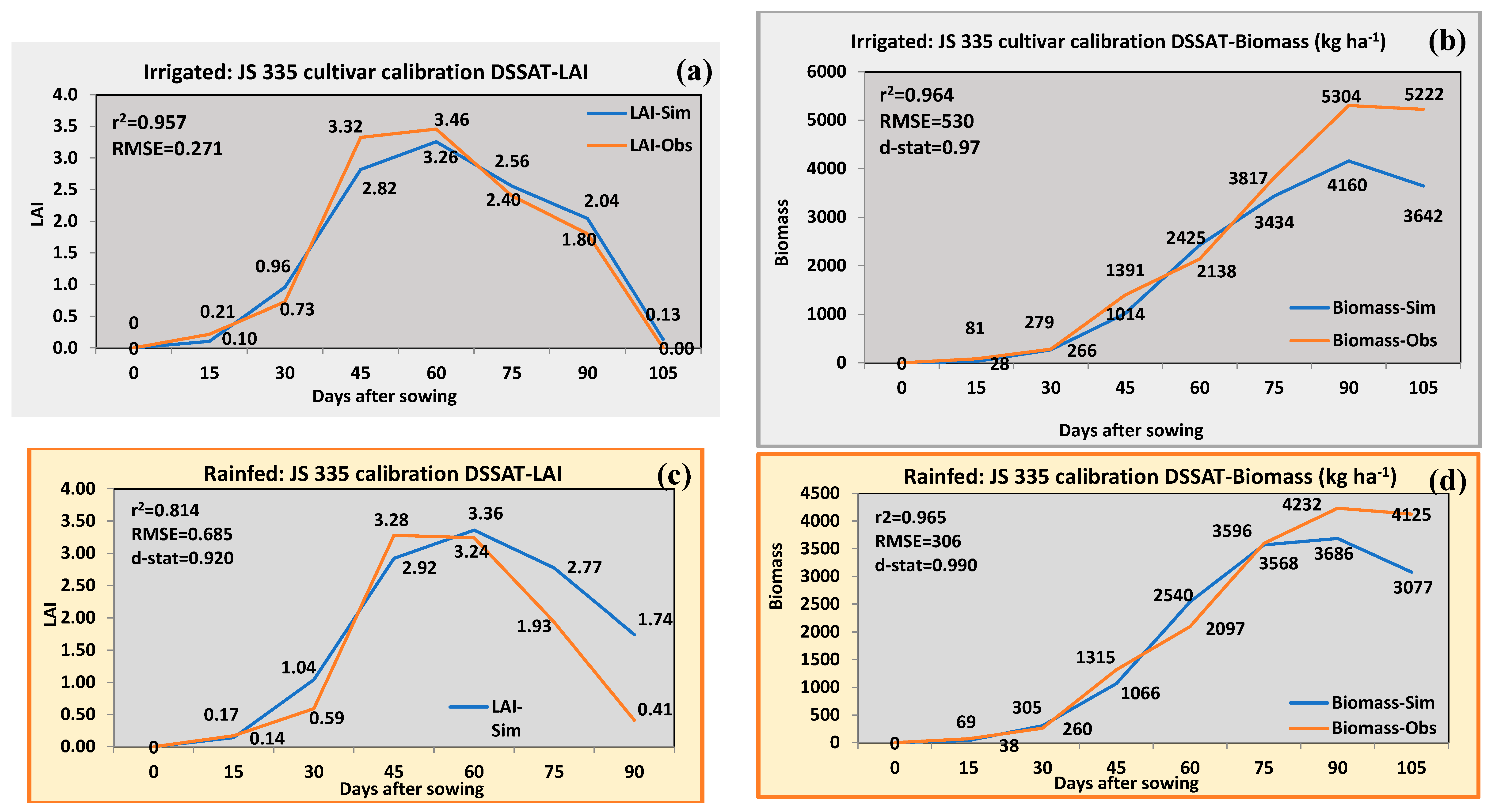
3.1. Model Calibration and Validation
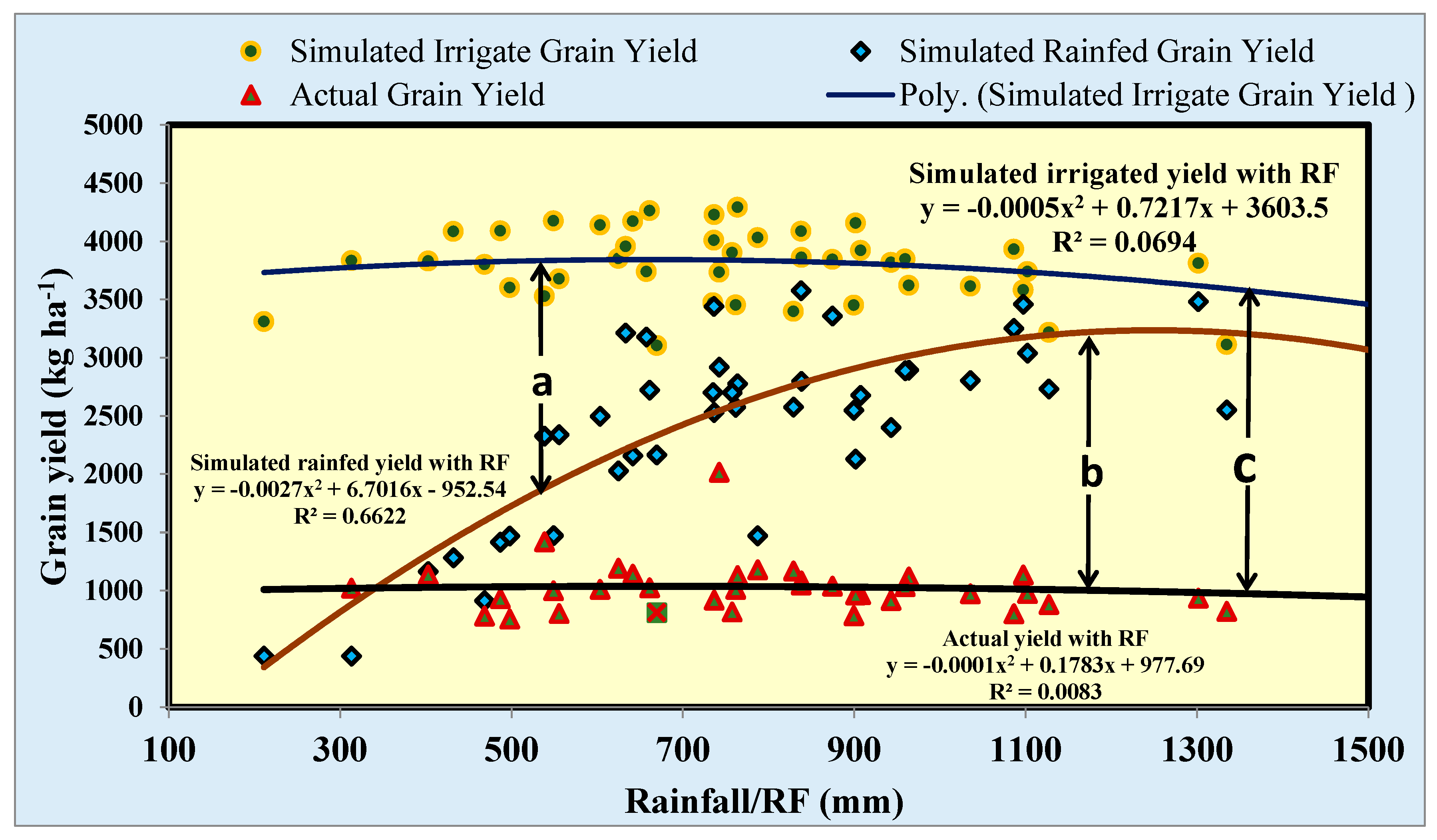
3.2. Simulated Yield under Irrigated Conditions
3.3. Simulated Yield under Rainfed Condition
3.4. Actual Yield of Soybean
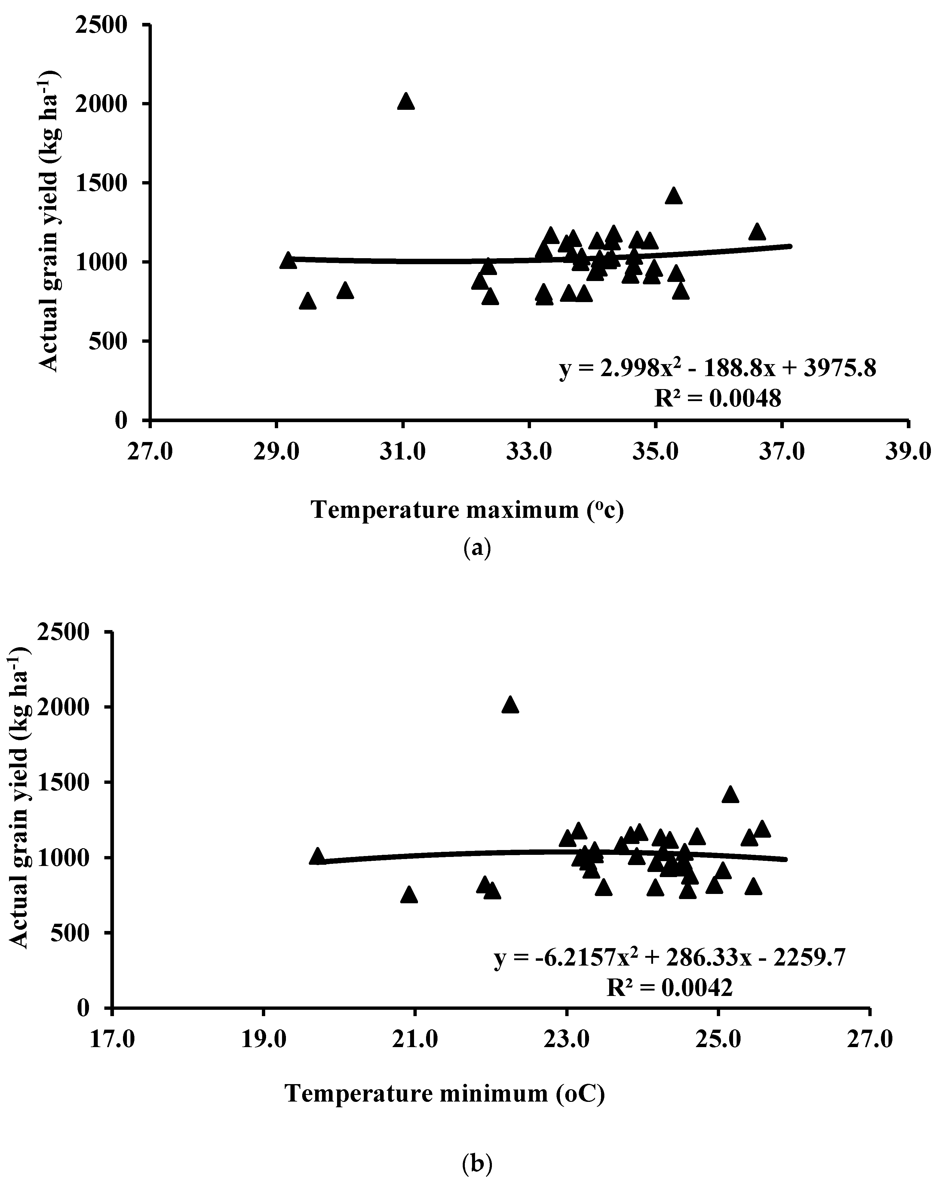
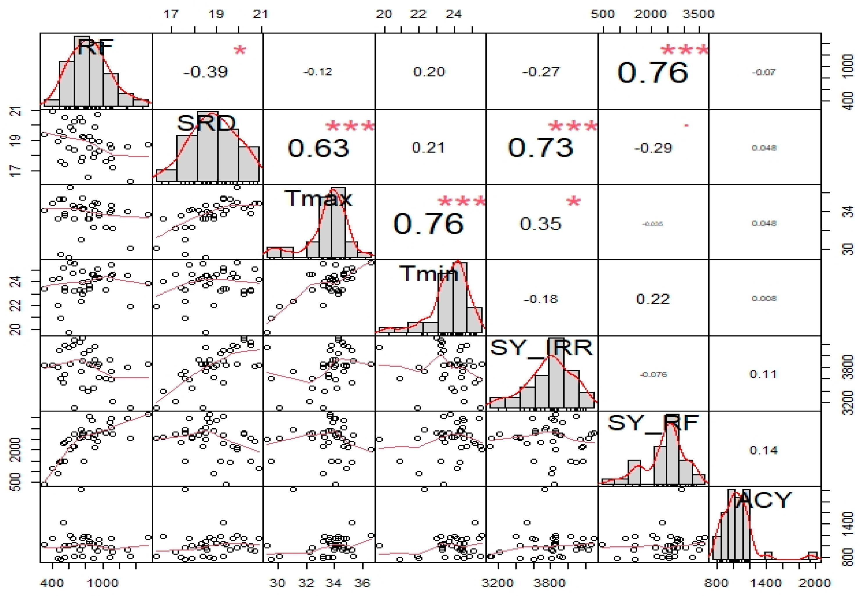
3.5. Climate Variability Effects on Soybean Yield
3.6. Yield Gaps of Soybean
4. Conclusions
Supplementary Materials
Author Contributions
Funding
Data Availability Statement
Acknowledgments
Conflicts of Interest
References
- Wani, S.P.; Rockström, J.; Oweis, T.Y. Rainfed Agriculture: Unlocking the Potential. In Comprehensive Assessment of Water Management in Agriculture Series; CABI: Wallingford, UK, 2009; ISBN 978-1-84593-389-0. [Google Scholar]
- Suresh, A.; Raju, S.S.; Chauhan, S.; Chaudhary, K.R. Rainfed Agriculture in India: An Analysis of Performance and Implications. Indian J. Agric. Sci. 2014, 84, 11. [Google Scholar] [CrossRef]
- Srinivasa Rao, C.; Lal, R.; Prasad, J.V.N.S.; Gopinath, K.A.; Singh, R.; Jakkula, V.S.; Sahrawat, K.L.; Venkateswarlu, B.; Sikka, A.K.; Virmani, S.M. Potential and Challenges of Rainfed Farming in India. In Advances in Agronomy; Elsevier: Amsterdam, The Netherlands, 2015; Volume 133, pp. 113–181. ISBN 978-0-12-803052-3. [Google Scholar]
- Bhatia, V.S.; Singh, P.; Wani, S.P.; Chauhan, G.S.; Rao, A.V.R.K.; Mishra, A.K.; Srinivas, K. Analysis of Potential Yields and Yield Gaps of Rainfed Soybean in India Using CROPGRO-Soybean Model. Agric. For. Meteorol. 2008, 148, 1252–1265. [Google Scholar] [CrossRef]
- Agarwal, D.K.; Billore, S.D.; Sharma, A.N.; Dupare, B.U.; Srivastava, S.K. Soybean: Introduction, Improvement, and Utilization in India—Problems and Prospects. Agric. Res. 2013, 2, 293–300. [Google Scholar] [CrossRef]
- Raghavendra, M.; Billore, S.D.; Verma, R.K. In-Situ Moisture Conservation and Residue Management for Soybean Production; Training Manual of Model Training Course on ‘Climate Resilient Technologies & Practices for Soybean Production’ organized during 4–11 September 2019; ICAR-Indian Institute of Soybean Research: Indore, India, 2019; pp. 110–115. Available online: https://iisrindore.icar.gov.in/ (accessed on 15 June 2024).
- Anderson, J.R. Rice Research in Asia: Progress and Priorities; Evenson, R.E., Herdt, R.W., Hossain, M., Eds.; CAB International: Wallingford, UK, 1996; Volume 17, pp. 289–290. ISBN 0-851-98997-7. [Google Scholar]
- Mohanty, M.; Sinha, N.K.; Patidar, R.K.; Somasundaram, J.; Chaudhary, R.S.; Hati, K.M.; Sammi Reddy, K.; Prabhakar, M.; Cherukumalli, S.R.; Patra, A.K. Assessment of Maize (Zea mays L.) Productivity and Yield Gap Analysis Using Simulation Modelling in Subtropical Climate of Central India. J. Agrometeorol. 2017, 19, 342–345. [Google Scholar] [CrossRef]
- Mohanty, M.; Sinha, N.K.; Lenka, S.; Hati, K.M.; Somasundaram, J.; Saha, R.; Singh, R.K.; Chaudhary, R.S.; Subba Rao, A. Climate Change Impacts on Rainfed Soybean Yield of Central India: Management Strategies Through Simulation Modelling. In Climate Change Modelling, Planning and Policy for Agriculture; Singh, A.K., Dagar, J.C., Arunachalam, A.R.G., Shelat, K.N., Eds.; Springer: New Delhi, India, 2015; pp. 39–44. ISBN 978-81-322-2156-2. [Google Scholar]
- Naab, J.B.; Singh, P.; Boote, K.J.; Jones, J.W.; Marfo, K.O. Using the CROPGRO-Peanut Model to Quantify Yield Gaps of Peanut in the Guinean Savanna Zone of Ghana. Agron. J. 2004, 96, 1231–1242. [Google Scholar] [CrossRef]
- Boote, K.J.; Jones, J.W.; Pickering, N.B. Potential Uses and Limitations of Crop Models. Agron. J. 1996, 88, 704–716. [Google Scholar] [CrossRef]
- Hoogenboom, G.; Wilkens, P.W.; Thornton, P.K.; Jones, J.W.; Hunt, L.A.; Imamura, D.T. Decision Support System for Agrotechnology Transfer v3. 5, DSSAT Version; Springer: Cham, Switzerland, 1999; Volume 3, pp. 1–36. [Google Scholar]
- Jones, J.W.; Hoogenboom, G.; Porter, C.H.; Boote, K.J.; Batchelor, W.D.; Hunt, L.A.; Wilkens, P.W.; Singh, U.; Gijsman, A.J.; Ritchie, J.T. The DSSAT Cropping System Model. Eur. J. Agron. 2003, 18, 235–265. [Google Scholar] [CrossRef]
- Boote, K.J.; Jones, J.W.; Hoogenboom, G.; Pickering, N.B. The CROPGRO Model for Grain Legumes. In Understanding Options for Agricultural Production; Tsuji, G.Y., Hoogenboom, G., Thornton, P.K., Eds.; Systems Approaches for Sustainable Agricultural Development; Springer: Dordrecht, The Netherlands, 1998; Volume 7, pp. 99–128. ISBN 978-90-481-4940-7. [Google Scholar]
- Bhatia, V.S.; Tiwari, S.P.; Sushil Pandey, S.P. Soybean Seed Quality Scenario in India—A Review. Seed Res. 2002, 30, 171–185. [Google Scholar]
- Dupare, B.U. Improved Technologies and Recommendations for Maximizing Soybean Productivity; Extension Bulletin No. 18; ICAR-Indian Institute of Soybean Research: Indore, India, 2023.
- Singh, P.; Boote, K.J.; Virmani, S.M. Evaluation of the Groundnut Model PNUTGRO for Crop Response to Plant Population and Row Spacing. Field Crops Res. 1994, 39, 163–170. [Google Scholar] [CrossRef]
- AICRP, R. All India Coordinated Research Project on Soybean, Directors Reports and Summary Tables of Experiments from Reports 2018; ICAR-Indian Institute of Soybean Research: Indore, India, 2018.
- Wallach, D.; Goffinet, B. Mean Squared Error of Prediction as a Criterion for Evaluating and Comparing System Models. Ecol. Model. 1989, 44, 299–306. [Google Scholar] [CrossRef]
- Willmott, C.J. Some Comments on the Evaluation of Model Performance. Bull. Am. Meteorol. Soc. 1982, 63, 1309–1313. [Google Scholar] [CrossRef]
- Peterson, B.G.; Carl, P.; Boudt, K.; Bennett, R.; Ulrich, J.; Zivot, E.; Cornilly, D.; Hung, E.; Lestel, M.; Balkissoon, K.; et al. Package ‘performanceanalytics’. R Team Coop. 2018, 3, 13–14. [Google Scholar]
- Lal, S.; Deshpande, S.B. Soil Series of India. In Soils Bulletin; National Bureau of Soil Survey and Land Use Planning: Nagpur, India, 1994; Volume 40. [Google Scholar]
- Bhatia, V.S.; Tiwari, S.P.; Joshi, O.P. Yield and Its Attributes as Affected by Planting Dates in Soybean (Glycine Max) Varieties. Indian J. Agric. Sci. 1999, 69, 696–699. [Google Scholar]
- Economics and Statistics, Ministry of Agriculture, Government of India. Available online: https://eands.da.gov.in/aboutus.htm (accessed on 15 June 2024).
- Adeboye, O.B.; Schultz, B.; Adekalu, K.O.; Prasad, K. Soil Water Storage, Yield, Water Productivity and Transpiration Efficiency of Soybeans (Glyxine Max L. Merr) as Affected by Soil Surface Management in Ile-Ife, Nigeria. Int. Soil Water Conserv. Res. 2017, 5, 141–150. [Google Scholar] [CrossRef]
- Ramesh, K.; Patra, A.K.; Biswas, A.K. Best Management Practices for Soybean under Soybean-Wheat System to Minimize the Impact of Climate Change. Indian J. Fertil. 2017, 12, 42–55. [Google Scholar]
- Bhatnagar, P.S.; Joshi, O.P. Current Status of Soybean Production and Utilization in India. In Proceedings of the VII World Soybean Research Conference, VI International Soybean Processing and Utilization Conference, III Congresso Brasileiro de Soja oz do Iguassu, Campinas, Brazil, 29 February–5 March 2004. [Google Scholar]
- Joshi, O.P.; Bhatia, V.S. Stress Management in Soybean. In Proceedings of the National Seminar on Stress Management in Oilseeds for Attaining Self-Reliance in Vegetable Oils, Hyderabad, India, 28–30 January 2003; Indian Society of Oilseeds Research: Hyderabad, India, 2003; pp. 13–25. [Google Scholar]
- Zheng, H.; Chen, L.; Han, X. Response of Soybean Yield to Daytime Temperature Change during Seed Filling: A Long-Term Field Study in Northeast China. Plant Prod. Sci. 2009, 12, 526–532. [Google Scholar] [CrossRef]
- Mishra, V.; Cherkauer, K.A. Retrospective Droughts in the Crop Growing Season: Implications to Corn and Soybean Yield in the Midwestern United States. Agric. For. Meteorol. 2010, 150, 1030–1045. [Google Scholar] [CrossRef]
- Onat, B.; Bakal, H.; Güllüoğlu, L.; Arioğlu, H. The Effects of High Temperature at the Growing Period on Yield and Yield Components of Soybean [Glycine Max (L.) Merr] Varieties. Turk. J. Field Crops 2017, 22, 178–186. [Google Scholar] [CrossRef]
- Billore, S.D.; Dupare, B.U.; Sharma, P. Addressing Climate Change Impact on Soybean through Resilient Technology. Soybean Res. 2018, 16, 1–24. [Google Scholar]
- Erkossa, T.; Stahr, K.; Gaiser, T. Soil Tillage and Crop Productivity on a Vertisol in Ethiopian Highlands. Soil Tillage Res. 2006, 85, 200–211. [Google Scholar] [CrossRef]
- Wani, S.P.; Pathak, P.; Sreedevi, T.K.; Singh, H.P.; Singh, P. Efficient Management of Rainwater for Increased Crop Productivity and Groundwater Recharge in Asia. In Water Productivity in Agriculture: Limits and Opportunities for Improvement; Kijne, J.W., Barker, R., Molden, D., Eds.; CAB International Publishing: Egham, UK, 2003; pp. 199–215. ISBN 978-0-85199-669-1. [Google Scholar]
- Jha, P.K.; Kumar, S.N.; Ines, A.V.M. Responses of Soybean to Water Stress and Supplemental Irrigation in Upper Indo-Gangetic Plain: Field Experiment and Modeling Approach. Field Crops Res. 2018, 219, 76–86. [Google Scholar] [CrossRef]
- Bhatia, V.S.; Singh, P.; Wani, S.P.; Rao, A.K.; Srinivas, K. Yield Gap Analysis of Soybean, Groundnut, Pigeonpea and Chickpea in India Using Simulation Modeling; Report no. 31; ICRISAT: Patancheruvu, India, 2006. [Google Scholar]


| S. No. | Cultivar Traits | Acronym | Unit | * Genetic Coefficients |
|---|---|---|---|---|
| 1 | Critical Short-Day Length below which reproductive development progresses with no day length effect | CSDL | h | 12.35 |
| 2 | Slope of the relative response of development to photoperiod with time | PPSEN | h−1 | 0.315 |
| 3 | Time between plant emergence and flower appearance (R1) | EM-FL | Photothermal days | 22 |
| 4 | Time between first flower and first pod (R3) | FL-SH | Photothermal days | 6.5 |
| 5 | Time between first flower and first seed (R5) | FL-SD | Photothermal days | 13 |
| 6 | Time between first seed (R5) and physiological maturity (R7) | SD-PM | Photothermal days | 32 |
| 7 | Time between first flower (R1) and end of leaf expansion | FL-LF | Photothermal days | 18 |
| 8 | Maximum leaf photosynthesis rate at 30 °C, 350 vpm CO2, and high light | LFMAX | mg Co2 m−2 s−1 | 1.03 |
| 9 | Specific leaf area of cultivar under standard growth conditions | SLAVR | cm2 g−1 | 400 |
| 10 | Maximum size of full leaf (three leaflets) | SIZLF | cm2 | 180 |
| 11 | Maximum fraction of daily growth that is partitioned to seed + shell | XFRT | 1.00 | |
| 12 | Maximum weight per seed | WTPSD | g | 0.15 |
| 13 | Seed filling duration for pod cohort at standard growth conditions | SFDUR | Photothermal days | 22 |
| 14 | Average seed per pod under standard growing conditions | SDPDV | Numbers per pod | 2.20 |
| 15 | Time required for cultivar to reach final pod load under optimal conditions | PODUR | Photothermal days | 7.5 |
| 16 | Threshing percentage. The maximum ratio of (seed/(seed + shell)) at maturity. Causes seeds to stop growing as their dry weight increases until shells are filled in a cohort. | THRSH | Percentage | 78 |
| 17 | Fraction protein in seeds | SDPRO | g protein g−1 seed | 0.400 |
| 18 | Fraction oil in seeds | SDLIP | g oil g−1 seed | 0.200 |
| S. No. | Location | State | Period | No. of Simulated Years | Latitude (°N) | Longitude (°E) | Soil Depth (CM) | Soil Water Extractable at Maturity (SWXM) |
|---|---|---|---|---|---|---|---|---|
| 1 | Amravati | Maharashtra | 1997–2017 | 21 | 20.9374 | 77.7796 | 240 | 187 |
| 2 | Betul | Madhya Pradesh | 1997–2018 | 22 | 21.9672 | 77.7452 | 240 | 253 |
| 3 | Dhar | Madhya Pradesh | 1997–2018 | 22 | 22.4959 | 75.1545 | 45.0 | 29.9 |
| 4 | Indore | Madhya Pradesh | 1997–2017 | 21 | 22.7196 | 75.8577 | 160 | 146 |
| 5 | Nagpur | Maharashtra | 1997–2018 | 22 | 21.1458 | 79.0882 | 140 | 134 |
| 6 | Rajgarh | Madhya Pradesh | 1997–2018 | 22 | 23.8509 | 76.7337 | 140 | 69.9 |
| 7 | Ratlam | Madhya Pradesh | 1997–2018 | 22 | 23.3342 | 75.0376 | 160 | 142 |
| 8 | Sagar | Madhya Pradesh | 1997–2018 | 22 | 25.8388 | 78.7378 | 140 | 126 |
| 9 | Sehore | Madhya Pradesh | 1997–2018 | 22 | 23.2050 | 77.0851 | 160 | 124 |
| 10 | Shajapur | Madhya Pradesh | 1997–2018 | 22 | 23.4186 | 76.5951 | 140 | 132 |
| 11 | Ujjain | Madhya Pradesh | 1997–2017 | 21 | 23.1793 | 75.7849 | 45.0 | 120 |
| 12 | Vidisha | Madhya Pradesh | 1997–2018 | 22 | 23.5251 | 77.8081 | 140 | 124 |
| 13 | Akola | Maharashtra | 1997–2018 | 22 | 20.7002 | 77.0082 | 240 | 181 |
| 14 | Bhopal | Madhya Pradesh | 1997–2017 | 21 | 23.2599 | 77.4126 | 140 | 122 |
| 15 | Guna | Madhya Pradesh | 1997–2018 | 22 | 24.6455 | 77.2865 | 77.0 | 52.6 |
| 16 | Hoshangabad | Madhya Pradesh | 1997–2018 | 22 | 22.7441 | 77.7370 | 140 | 137 |
| 17 | Kota | Rajasthan | 1997–2018 | 22 | 25.2138 | 75.8648 | 188 | 98 |
| 18 | Nanded | Maharashtra | 1997–2018 | 22 | 19.1383 | 77.3210 | 240 | 216 |
| 19 | Neemuch | Madhya Pradesh | 1997–2018 | 22 | 24.4764 | 74.8624 | 140 | 102 |
| 20 | Parbhani | Maharashtra | 1997–2018 | 22 | 19.2644 | 76.6413 | 140 | 125 |
| 21 | Wardha | Maharashtra | 1997–2018 | 22 | 20.7453 | 78.6022 | 150 | 127 |
| 22 | Belagavi | Karnataka | 1997–2018 | 22 | 15.8497 | 74.4977 | 170 | 171 |
| 23 | Dharwad | Karnataka | 1997–2018 | 22 | 15.4589 | 75.0078 | 170 | 86.6 |
| 24 | Gulbarga | Karnataka | 1997–2018 | 22 | 17.3297 | 76.8343 | 200 | 127 |
| 25 | Jabalpur | Madhya Pradesh | 1997–2018 | 22 | 23.1815 | 79.9864 | 180 | 189 |
| 26 | Jhabua | Madhya Pradesh | 1997–2018 | 22 | 22.9159 | 74.6869 | 160 | 154 |
| 27 | Anantapur | Andhra Pradesh | 1997–2018 | 22 | 14.6819 | 77.6006 | 156 | 74.7 |
| 28 | Bangalore | Karnataka | 1997–2018 | 22 | 12.9716 | 77.5946 | 146 | 93.3 |
| 29 | Bellary | Karnataka | 1997–2018 | 22 | 15.1394 | 76.9214 | 170 | 47.7 |
| 30 | Bijapur | Karnataka | 1997–2018 | 22 | 18.8608 | 80.7214 | 170 | 79.3 |
| 31 | Coimbatore | Tamil Nadu | 1997–2018 | 22 | 11.0168 | 76.9558 | 124 | 27.2 |
| 32 | Faizabad | Uttar Pradesh | 1997–2018 | 22 | 26.7730 | 82.1458 | 128 | 105 |
| 33 | Hissar | Haryana | 1997–2018 | 22 | 29.1492 | 75.7217 | 168 | 57.6 |
| 34 | Hyderabad | Telangana state | 1997–2018 | 22 | 17.3850 | 78.4867 | 202 | 83.5 |
| 35 | Junagarh | Gujrat | 1997–2018 | 22 | 21.5222 | 70.4579 | 120 | 68.0 |
| 36 | Kanpur | Uttar Pradesh | 1997–2018 | 22 | 26.4499 | 80.3319 | 156 | 63.6 |
| 37 | Karnool | Andhra Pradesh | 1997–2018 | 22 | 15.8281 | 78.0373 | 150 | 89.1 |
| 38 | Ludhiana | Punjab | 1997–2018 | 22 | 30.9010 | 75.8573 | 165 | 73.0 |
| 39 | New Delhi | Uttarakhand | 1997–2018 | 22 | 28.6139 | 77.2090 | 165 | 69.1 |
| 40 | Pantnagar | Uttarakhand | 1997–2018 | 22 | 28.9610 | 79.5154 | 128 | 109 |
| 41 | Pune | Maharashtra | 1997–2018 | 22 | 18.5200 | 73.8500 | 150 | 104 |
| 42 | Raichur | Karnataka | 1997–2018 | 22 | 16.2008 | 77.3622 | 150 | 125 |
| 43 | Raipur | Chhattisgarh | 1997–2018 | 22 | 21.2514 | 81.6296 | 160 | 166 |
| Years | Rainfed JS 335 | Irrigated JS 335 | ||||||
|---|---|---|---|---|---|---|---|---|
| GY_Obs | GY_Sim | BY_Obs | BY_Sim | GY_Obs | GY_Sim | BY_Obs | BY_Sim | |
| (kg ha−1) | (kg ha−1) | (kg ha−1) | (kg ha−1) | (kg ha−1) | (kg ha−1) | (kg ha−1) | (kg ha−1) | |
| 2013 | 661 | 1689 | 3248 | 4339 | 883 | 1801 | 3771 | 4560 |
| 2014 | 628 | 1714 | 4008 | 4829 | 950 | 1816 | 4321 | 5103 |
| RMSE | 1057 | 965 | 892 | 786 | ||||
| S. No. | Locations | Simulated Potential Yield (kg ha−1) | Actual Yield (kg ha−1) (C) | Yield Gap (kg ha−1) | |||||||||
|---|---|---|---|---|---|---|---|---|---|---|---|---|---|
| Irrigated (Water Non-Limiting) | Rainfed (Water Limiting) | Water Limitation (A − B) | Factor Other than Water Availability (B − C) | Total (A − C) | |||||||||
| Min | Max | Mean (A) | CV | Min | Max | Mean (B) | CV | ||||||
| 1 | Amravati | 3335 | 4979 | 4262 | 10.2 | 0 | 4563 | 2722 | 35.1 | 1025 | 1540 | 1697 | 3237 |
| 2 | Betul | 2525 | 4051 | 3615 | 10.5 | 1753 | 3485 | 2805 | 18.6 | 974 | 810 | 1831 | 2640 |
| 3 | Dhar | 2853 | 5293 | 4031 | 17.6 | 509 | 2284 | 1472 | 36.2 | 1181 | 2559 | 292 | 2850 |
| 4 | Indore | 2162 | 4214 | 3398 | 20.0 | 1431 | 3634 | 2576 | 29.0 | 1170 | 822 | 1406 | 2228 |
| 5 | Nagpur | 3222 | 4127 | 3818 | 6.10 | 882 | 3529 | 2401 | 29.1 | 916 | 1417 | 1484 | 2902 |
| 6 | Rajgarh | 2485 | 4829 | 4089 | 12.5 | 0 | 4127 | 1417 | 107.9 | 931 | 2672 | 487 | 3159 |
| 7 | Ratlam | 2705 | 4497 | 3862 | 11.8 | 1584 | 3971 | 2798 | 25.3 | 1085 | 1064 | 1713 | 2777 |
| 8 | Sagar | 2254 | 4418 | 3931 | 10.8 | 1910 | 3921 | 3253 | 17.8 | 803 | 678 | 2450 | 3128 |
| 9 | Shajapur | 2575 | 4402 | 3922 | 8.9 | 893 | 3691 | 2677 | 27.2 | 965 | 1245 | 1712 | 2957 |
| 10 | Sehore | 2536 | 4223 | 3621 | 11.9 | 1114 | 3763 | 2894 | 25.3 | 1118 | 727 | 1776 | 2503 |
| 11 | Ujjain | 3052 | 4790 | 4086 | 10.2 | 2271 | 4292 | 3576 | 12.5 | 1050 | 510 | 2526 | 3036 |
| 12 | Vidisha | 2371 | 4256 | 3739 | 11.6 | 1542 | 4075 | 3039 | 19.9 | 975 | 700 | 2064 | 2764 |
| 13 | Akola | 2809 | 4569 | 4172 | 9.27 | 1225 | 3532 | 2157 | 31.1 | 1142 | 2015 | 1015 | 3030 |
| 14 | Bhopal | 2856 | 4244 | 3848 | 9.10 | 1253 | 3860 | 2889 | 28.2 | 1036 | 959 | 1853 | 2812 |
| 15 | Guna | 3764 | 4562 | 4156 | 4.44 | 648 | 3548 | 2131 | 35.9 | 963 | 2025 | 1168 | 3193 |
| 16 | Hoshangabad | 2444 | 3836 | 3217 | 12.4 | 1647 | 3490 | 2732 | 18.8 | 881 | 485 | 1851 | 2336 |
| 17 | Kota | 3099 | 4330 | 3853 | 7.74 | 539 | 3833 | 2029 | 50.6 | 1193 | 1824 | 835 | 2659 |
| 18 | Nanded | 2954 | 3859 | 3453 | 7.04 | 1558 | 3621 | 2575 | 23.9 | 1011 | 878 | 1563 | 2442 |
| 19 | Neemuch | 3327 | 5069 | 4228 | 11.0 | 391 | 4044 | 2530 | 38.3 | 920 | 1698 | 1610 | 3308 |
| 20 | Parbhani | 3880 | 4838 | 4292 | 5.93 | 1566 | 3947 | 2777 | 25.9 | 1131 | 1515 | 1647 | 3161 |
| 21 | Wardha | 2700 | 4890 | 3843 | 14.3 | 1452 | 4688 | 3359 | 18.9 | 1039 | 485 | 2319 | 2804 |
| 22 | Belagavi | 2462 | 3529 | 3114 | 9.16 | 1087 | 3134 | 2553 | 18.6 | 823 | 561 | 1730 | 2290 |
| 23 | Dharwad | 3217 | 3990 | 3602 | 5.10 | 0 | 3320 | 1470 | 72.3 | 756 | 2131 | 714 | 2846 |
| 24 | Gulbarga | 3283 | 4037 | 3678 | 6.68 | 0 | 3652 | 2339 | 40.2 | 805 | 1339 | 1534 | 2873 |
| 25 | Jabalpur | 2446 | 4467 | 3811 | 11.9 | 2365 | 4220 | 3482 | 12.8 | 936 | 329 | 2546 | 2875 |
| 26 | Jhabua | 2538 | 3878 | 3452 | 9.50 | 1473 | 3446 | 2549 | 22.2 | 785 | 903 | 1764 | 2667 |
| 27 | Anantpur | 3478 | 4159 | 3831 | 5.22 | 247 | 3059 | 1164 | 64.0 | 1136 | 2667 | 29 | 2695 |
| 28 | Bangalore | 3731 | 4559 | 4140 | 4.58 | 939 | 3702 | 2498 | 27.6 | 1012 | 1642 | 1486 | 3128 |
| 29 | Bellary | 3321 | 4874 | 3834 | 9.63 | 0 | 1229 | 439 | 88.4 | 1022 | 3395 | −583 | 2812 |
| 30 | Bijapur | 2611 | 4561 | 3802 | 12.5 | 0 | 3041 | 915 | 78.7 | 782 | 2887 | 133 | 3020 |
| 31 | Coimbatore | 2618 | 3662 | 3310 | 7.43 | 0 | 1736 | 438 | 81.6 | * | 2872 | - | - |
| 32 | Faizabad | 3543 | 4292 | 4010 | 5.92 | 748 | 4166 | 3442 | 24.5 | * | 568 | - | - |
| 33 | Hissar | 3481 | 4317 | 4085 | 4.73 | 4 | 3696 | 1283 | 76.7 | * | 2802 | - | - |
| 34 | Hyderabad | 2995 | 3953 | 3472 | 6.28 | 214 | 3616 | 2702 | 30.1 | * | 770 | - | - |
| 35 | Junagarh | 2687 | 3549 | 3104 | 6.36 | 4 | 3029 | 2166 | 40.0 | 811 | 939 | 1354 | 2293 |
| 36 | Kanpur | 3022 | 4734 | 3902 | 8.45 | 984 | 3705 | 2700 | 29.7 | 819 | 1202 | 1881 | 3083 |
| 37 | Kurnool | 3259 | 3881 | 3528 | 3.79 | 431 | 3483 | 2327 | 49.2 | 1421 | 1201 | 906 | 2107 |
| 38 | Ludhiana | 3632 | 4399 | 3956 | 4.41 | 1901 | 3923 | 3213 | 21.3 | * | 742 | - | - |
| 39 | New Delhi | 2187 | 4082 | 3740 | 10.9 | 1673 | 3978 | 3178 | 22.7 | * | 562 | - | - |
| 40 | Pantnagar | 3409 | 4142 | 3852 | 5.98 | 2901 | 4022 | 3663 | 7.97 | 1151 | 189 | 2512 | 2702 |
| 41 | Pune | 2613 | 4265 | 3734 | 8.70 | 1436 | 3910 | 2920 | 24.5 | 2018 | 815 | 902 | 1716 |
| 42 | Raichur | 3537 | 5023 | 4175 | 7.54 | 167 | 3482 | 1473 | 54.7 | 1000 | 2701 | 473 | 3175 |
| 43 | Raipur | 2748 | 3853 | 3582 | 6.33 | 2667 | 3730 | 3460 | 6.73 | 1135 | 122 | 2325 | 2447 |
| Average | 2947 | 4337 | 3794 | 8.94 | 1010 | 3609 | 2446 | 36.0 | 1025 | 1348 | 1433 | 2775 | |
| CV a | 15.8 | 9.79 | 8.02 | 39.2 | 80.0 | 17.7 | 33.4 | 64.3 | 21.7 | 64.1 | 52.7 | 12.9 | |
| S. No | Locations | Solar Radiation (MJm−2 day−1) | Maximum Temperature (°C) | Minimum Temperature (°C) | |||||||||
|---|---|---|---|---|---|---|---|---|---|---|---|---|---|
| Min | Max | Mean | CV | Min | Max | Mean | CV | Min | Max | Mean | CV | ||
| 1 | Amravati | 17.0 | 24.4 | 20.2 | 9.60 | 31.5 | 36.9 | 34.3 | 3.31 | 18.9 | 25.3 | 23.2 | 7.43 |
| 2 | Betul | 15.7 | 19.0 | 17.6 | 5.56 | 30.9 | 33.7 | 32.4 | 2.23 | 22.5 | 24.2 | 23.3 | 2.01 |
| 3 | Dhar | 16.1 | 22.0 | 19.2 | 7.82 | 29.0 | 35.9 | 34.3 | 3.93 | 19.4 | 24.7 | 23.2 | 5.71 |
| 4 | Indore | 10.8 | 20.9 | 16.6 | 18.2 | 30.4 | 35.0 | 33.3 | 3.43 | 23.0 | 24.7 | 24.0 | 1.87 |
| 5 | Nagpur | 18.2 | 22.6 | 20.7 | 8.51 | 33.1 | 36.3 | 34.9 | 2.02 | 24.3 | 25.8 | 25.1 | 1.61 |
| 6 | Rajgarh | 16.9 | 23.6 | 19.6 | 9.79 | 31.3 | 39.6 | 35.3 | 4.60 | 21.0 | 26.7 | 24.3 | 6.08 |
| 7 | Ratlam | 15.5 | 20.9 | 18.5 | 7.06 | 31.1 | 35.3 | 33.2 | 2.52 | 22.6 | 24.6 | 23.7 | 1.92 |
| 8 | Sagar | 16.3 | 20.8 | 18.7 | 5.07 | 31.6 | 35.1 | 33.9 | 2.33 | 23.3 | 24.9 | 24.2 | 1.83 |
| 9 | Shajapur | 15.6 | 20.9 | 18.2 | 6.65 | 32.7 | 35.7 | 34.1 | 2.21 | 23.3 | 24.9 | 24.2 | 1.54 |
| 10 | Sehore | 16.8 | 20.4 | 18.9 | 5.23 | 0.0 | 38.1 | 33.6 | 17.9 | 23.7 | 25.0 | 24.4 | 1.34 |
| 11 | Ujjain | 17.1 | 21.5 | 19.3 | 6.45 | 32.2 | 35.8 | 33.7 | 2.32 | 21.7 | 24.5 | 23.4 | 3.12 |
| 12 | Vidisha | 15.8 | 20.5 | 18.5 | 7.22 | 32.8 | 37.0 | 34.7 | 3.07 | 22.5 | 25.3 | 24.5 | 2.21 |
| 13 | Akola | 16.2 | 20.8 | 19.7 | 6.04 | 33.1 | 36.0 | 34.7 | 2.35 | 23.8 | 25.4 | 24.7 | 1.98 |
| 14 | Bhopal | 16.9 | 19.4 | 18.3 | 4.59 | 31.6 | 35.6 | 33.8 | 2.33 | 23.0 | 24.9 | 24.3 | 2.00 |
| 15 | Guna | 18.5 | 21.3 | 19.9 | 3.42 | 32.9 | 37.0 | 35.0 | 2.29 | 23.2 | 25.2 | 24.4 | 2.19 |
| 16 | Hoshangabad | 15.1 | 18.5 | 17.2 | 5.94 | 0.0 | 35.5 | 32.2 | 25.5 | 23.8 | 25.6 | 24.6 | 1.78 |
| 17 | Kota | 18.2 | 22.7 | 19.9 | 6.12 | 35.0 | 39.7 | 36.6 | 3.05 | 24.8 | 26.4 | 25.6 | 1.68 |
| 18 | Nanded | 15.5 | 19.9 | 17.9 | 5.50 | 30.7 | 37.3 | 34.2 | 3.31 | 22.1 | 24.8 | 23.9 | 2.74 |
| 19 | Neemuch | 17.4 | 23.4 | 20.5 | 8.58 | 33.2 | 37.1 | 34.6 | 2.37 | 19.8 | 25.1 | 23.3 | 7.55 |
| 20 | Parbhani | 18.6 | 22.0 | 20.2 | 4.81 | 32.7 | 35.4 | 34.3 | 2.10 | 21.3 | 23.9 | 23.0 | 2.90 |
| 21 | Wardha | 15.1 | 23.3 | 19.0 | 10.7 | 32.7 | 36.5 | 34.7 | 2.54 | 20.0 | 26.9 | 24.6 | 6.00 |
| 22 | Belagavi | 14.6 | 18.2 | 16.3 | 5.30 | 27.7 | 36.6 | 30.1 | 8.22 | 20.4 | 23.1 | 21.9 | 4.42 |
| 23 | Dharwad | 16.5 | 18.9 | 17.6 | 3.04 | 28.3 | 31.5 | 29.5 | 2.07 | 20.3 | 21.5 | 20.9 | 1.61 |
| 24 | Gulbarga | 16.1 | 18.8 | 17.4 | 4.37 | 31.8 | 36.3 | 33.6 | 2.62 | 22.7 | 24.6 | 23.5 | 1.88 |
| 25 | Jabalpur | 16.7 | 20.4 | 18.6 | 5.76 | 31.9 | 35.6 | 34.0 | 2.24 | 23.2 | 25.4 | 24.5 | 2.34 |
| 26 | Jhabua | 15.5 | 19.2 | 17.9 | 6.35 | 0.0 | 36.2 | 32.4 | 25.5 | 23.9 | 25.7 | 24.6 | 2.02 |
| 27 | Anantpur | 18.5 | 23.1 | 20.9 | 6.35 | 33.3 | 36.3 | 34.9 | 1.74 | 22.7 | 25.4 | 24.2 | 2.48 |
| 28 | Bangalore | 17.3 | 19.4 | 18.5 | 2.76 | 28.1 | 30.2 | 29.2 | 1.80 | 19.1 | 20.2 | 19.7 | 1.65 |
| 29 | Bellary | 16.7 | 25.9 | 19.4 | 9.71 | 32.1 | 37.3 | 34.1 | 2.74 | 17.2 | 26.4 | 23.4 | 7.79 |
| 30 | Bijapur | 15.9 | 21.4 | 18.9 | 7.68 | 31.8 | 36.0 | 33.2 | 2.98 | 20.8 | 23.3 | 22.0 | 2.53 |
| 31 | Coimbatore | 16.0 | 20.9 | 18.3 | 5.40 | 28.0 | 33.6 | 32.3 | 2.73 | 20.8 | 23.7 | 22.9 | 2.54 |
| 32 | Faizabad | 17.4 | 23.3 | 19.1 | 6.13 | 33.0 | 36.5 | 34.6 | 2.24 | 23.6 | 26.8 | 25.1 | 3.09 |
| 33 | Hissar | 18.8 | 22.3 | 20.7 | 4.24 | 35.6 | 39.1 | 37.1 | 2.28 | 22.9 | 26.6 | 24.6 | 3.59 |
| 34 | Hyderabad | 15.6 | 19.2 | 16.9 | 4.99 | 30.6 | 33.9 | 32.7 | 2.05 | 19.9 | 23.7 | 22.6 | 3.99 |
| 35 | Junagarh | 16.3 | 20.7 | 18.4 | 5.21 | 0.0 | 36.4 | 33.2 | 17.9 | 25.1 | 26.0 | 25.5 | 0.87 |
| 36 | Kanpur | 18.0 | 22.5 | 19.3 | 6.00 | 34.0 | 37.4 | 35.4 | 2.51 | 21.4 | 27.4 | 24.9 | 6.64 |
| 37 | Kurnool | 18.5 | 20.2 | 19.3 | 2.44 | 34.1 | 36.5 | 35.3 | 2.14 | 24.0 | 26.0 | 25.2 | 2.12 |
| 38 | Ludhiana | 18.3 | 23.4 | 19.9 | 7.11 | 0.0 | 38.1 | 34.4 | 17.9 | 23.9 | 25.9 | 25.0 | 1.82 |
| 39 | New Delhi | 9.7 | 20.6 | 18.5 | 11.7 | 0.0 | 39.3 | 35.2 | 17.9 | 24.3 | 26.8 | 25.9 | 2.20 |
| 40 | Pantnagar | 17.0 | 21.1 | 18.7 | 5.30 | 31.7 | 35.0 | 33.7 | 2.60 | 20.2 | 24.8 | 23.8 | 4.01 |
| 41 | Pune | 14.8 | 18.9 | 17.6 | 5.07 | 29.5 | 32.5 | 31.0 | 2.25 | 21.5 | 22.9 | 22.3 | 1.49 |
| 42 | Raichur | 18.1 | 23.4 | 20.5 | 6.37 | 0.0 | 37.1 | 33.8 | 17.8 | 19.3 | 24.6 | 23.2 | 4.91 |
| 43 | Raipur | 17.0 | 18.9 | 17.8 | 2.72 | 29.4 | 36.8 | 34.1 | 3.54 | 24.5 | 26.3 | 25.4 | 1.85 |
| Average | 16.4 | 21.2 | 18.8 | 6.44 | 26.5 | 36.1 | 33.8 | 5.57 | 22.1 | 25.0 | 23.9 | 3.05 | |
| CV a | 10.9 | 8.52 | 6.07 | 43.3 | 45.1 | 5.31 | 4.79 | 120 | 8.56 | 5.66 | 5.22 | 61.1 | |
| S. No. | Locations | Years | Reasons for Crop Failure | * AICRP Experiment Yield (kg ha−1) | * FLDs Yield (kg ha−1) | ** Actual/ District Yield (kg ha−1) |
|---|---|---|---|---|---|---|
| 1 | Amravati | 2009 | During 2011, rainfall data was not available. Whereas, in 2009, only 30 mm seasonal total rainfall was recorded. | 1611 | 800 | 809 |
| 2011 | 848 | 1452 | 1258 | |||
| 2 | Rajgarh | 2002 | During 2008 and 2011 rainfall data was not available. However, in 2002, 2003, and 2004 meager amount of total seasonal rainfall was received (11–21 mm) | - | - | 341 |
| 2003 | - | - | 1135 | |||
| 2004 | - | - | 885 | |||
| 2008 | - | - | 1087 | |||
| 2011 | - | - | 856 | |||
| 3 | Hoshangabad | 2017 | Weather data not available | - | - | - |
| 2018 | - | - | - | |||
| 4 | Dharwad | 2003 | Meager amount of total seasonal rainfall received (46 mm) | - | - | 638 |
| 5 | Gulbarga | 2008 | Meager amount of total seasonal rainfall received (181 mm) | - | - | 690 |
| 6 | Jhabua | 2017 | Weather data not available | - | - | - |
| 2018 | - | - | - | |||
| 7 | Bellary | 2001 | Meager amount of total seasonal rainfall was received (103.5 mm in 2001, 8.5mm in 2003 and 19.5 mm in 2006) | - | - | - |
| 2003 | - | - | - | |||
| 2006 | - | - | - | |||
| 8 | Bijapur | 1997 | During 1997 rainfall data was not available. In the remaining years 2001 and 2003 meager amount of seasonal rainfall was received (28–37 mm) | - | - | - |
| 2001 | - | - | - | |||
| 2003 | - | - | - | |||
| 9 | Coimbatore | 2012 | Meager amount of total seasonal rainfall was received (20 mm) | - | - | - |
| 10 | Junagarh | 2018 | Weather data not available | - | - | - |
| 11 | Ludhiana | 2016 | Weather data not available | - | - | - |
| 12 | New Delhi | 2005 | Weather data not available | - | - | - |
| S. No. | Location | Seasonal Rainfall | Season Surface Runoff | Season Water Drainage | |||||||||
|---|---|---|---|---|---|---|---|---|---|---|---|---|---|
| Min | Max | Mean | CV | Min | Max | Mean | CV | Min | Max | Mean | CV | ||
| 1 | Amravati | 0 | 980 | 661 | 41.1 | 0 | 306 | 166 | 50.0 | 0 | 171 | 19 | 235 |
| 2 | Betul | 624 | 1604 | 1035 | 23.0 | 126 | 672 | 313 | 47.4 | 0 | 432 | 176 | 69.8 |
| 3 | Dhar | 442 | 1181 | 787 | 23.7 | 47 | 421 | 216 | 50.1 | 60 | 499 | 250 | 40.2 |
| 4 | Indore | 483 | 1124 | 829 | 22.9 | 92 | 495 | 285 | 34.8 | 0 | 252 | 78 | 103 |
| 5 | Nagpur | 652 | 1278 | 943 | 19.0 | 137 | 531 | 312 | 35.6 | 0 | 247 | 101 | 62.7 |
| 6 | Rajgarh | 0 | 1380 | 487 | 101.2 | 0 | 516 | 139 | 116 | 0 | 488 | 127 | 127 |
| 7 | Ratlam | 480 | 1175 | 838 | 23.3 | 65 | 402 | 222 | 43.5 | 0 | 320 | 116 | 87.7 |
| 8 | Sagar | 628 | 1925 | 1086 | 30.8 | 112 | 927 | 370 | 53.1 | 0 | 668 | 223 | 71.2 |
| 9 | Shajapur | 405 | 1943 | 907 | 36.8 | 98 | 1013 | 299 | 68.5 | 0 | 444 | 122 | 110 |
| 10 | Sehore | 709 | 1492 | 964 | 24.7 | 89 | 516 | 233 | 50.2 | 67 | 509 | 248 | 53.9 |
| 11 | Ujjain | 483 | 1150 | 838 | 26.4 | 9 | 272 | 130 | 60.2 | 94 | 596 | 312 | 49.6 |
| 12 | Vidisha | 616 | 1938 | 1102 | 28.4 | 127 | 679 | 311 | 46.4 | 59 | 705 | 304 | 57.6 |
| 13 | Akola | 352 | 1021 | 642 | 27.1 | 42 | 343 | 167 | 46.4 | 0 | 123 | 12 | 254 |
| 14 | Bhopal | 598 | 1603 | 959 | 27.4 | 142 | 740 | 337 | 43.2 | 4 | 497 | 156 | 79.1 |
| 15 | Guna | 410 | 1491 | 901 | 29.7 | 72 | 648 | 322 | 49.3 | 34 | 465 | 207 | 53.9 |
| 16 | Hoshangabad | 782 | 1644 | 1127 | 24.3 | 150 | 568 | 320 | 38.8 | 174 | 626 | 343 | 44.4 |
| 17 | Kota | 310 | 1053 | 625 | 28.5 | 42 | 247 | 124 | 49.0 | 0 | 269 | 44 | 156 |
| 18 | Nanded | 517 | 1043 | 762 | 20.0 | 64 | 450 | 163 | 71.1 | 0 | 189 | 37 | 172 |
| 19 | Neemuch | 288 | 1353 | 736 | 30.0 | 48 | 634 | 187 | 65.7 | 0 | 344 | 108 | 89.2 |
| 20 | Parbhani | 430 | 1195 | 764 | 27.5 | 60 | 501 | 220 | 52.1 | 0 | 228 | 65 | 114 |
| 21 | Wardha | 370 | 1308 | 874 | 23.2 | 82 | 565 | 207 | 49.9 | 11 | 432 | 242 | 44.5 |
| 22 | Belagavi | 517 | 2180 | 1335 | 33.6 | 94 | 648 | 333 | 44.9 | 0 | 921 | 447 | 65.1 |
| 23 | Dharwad | 46 | 857 | 498 | 43.7 | 0 | 189 | 84 | 63.0 | 0 | 86 | 9 | 248 |
| 24 | Gulbarga | 181 | 782 | 555 | 28.8 | 10 | 84 | 40 | 58.1 | 0 | 91 | 11 | 224 |
| 25 | Jabalpur | 799 | 2099 | 1301 | 28.0 | 137 | 893 | 462 | 46.2 | 34 | 624 | 298 | 56.2 |
| 26 | Jhabua | 639 | 1209 | 899 | 21.1 | 137 | 351 | 237 | 30.2 | 0 | 330 | 157 | 66.8 |
| 27 | Anantpur | 112 | 727 | 403 | 39.4 | 0 | 97 | 20 | 124 | 106 | 343 | 202 | 36.6 |
| 28 | Bangalore | 281 | 899 | 603 | 26.1 | 5 | 143 | 56 | 66.6 | 181 | 503 | 358 | 24.0 |
| 29 | Bellary | 9 | 574 | 313 | 48.9 | 0 | 165 | 31 | 121 | 0 | 0 | 0 | - |
| 30 | Bijapur | 0 | 1047 | 468 | 51.0 | 0 | 345 | 100 | 78.0 | 0 | 148 | 7 | 469 |
| 31 | Coimbatore | 20 | 920 | 211 | 87.5 | 0 | 149 | 25 | 139 | 0 | 246 | 13 | 409 |
| 32 | Faizabad | 337 | 1185 | 736 | 37.6 | 8 | 319 | 114 | 74.8 | 48 | 558 | 279 | 56.7 |
| 33 | Hissar | 124 | 710 | 432 | 35.6 | 10 | 274 | 106 | 63.9 | 0 | 44 | 6 | 194 |
| 34 | Hyderabad | 293 | 1412 | 735 | 37.1 | 32 | 824 | 238 | 70.7 | 0 | 0 | 0 | - |
| 35 | Junagarh | 155 | 1358 | 669 | 44.3 | 21 | 559 | 198 | 66.9 | 0 | 393 | 98 | 110 |
| 36 | Kanpur Dehat | 379 | 1368 | 757 | 31.7 | 7 | 251 | 67 | 90.4 | 118 | 818 | 418 | 38.3 |
| 37 | Kurnool | 250 | 832 | 538 | 26.7 | 11 | 228 | 98 | 55.6 | 0 | 0 | 0 | - |
| 38 | Ludhiana | 310 | 974 | 633 | 32.3 | 14 | 285 | 108 | 73.0 | 168 | 486 | 311 | 32.1 |
| 39 | New Delhi | 384 | 1034 | 657 | 26.5 | 18 | 297 | 168 | 46.4 | 47 | 434 | 171 | 51.0 |
| 40 | Pantnagar | 694 | 2999 | 1535 | 37.9 | 144 | 1114 | 433 | 56.5 | 266 | 1381 | 691 | 46.1 |
| 41 | Pune | 362 | 1904 | 742 | 47.4 | 17 | 386 | 127 | 67.4 | 174 | 1331 | 415 | 60.8 |
| 42 | Raichur | 305 | 813 | 549 | 25.5 | 15 | 243 | 84 | 64.5 | 0 | 96 | 17 | 181 |
| 43 | Raipur | 710 | 1522 | 1097 | 21.2 | 97 | 461 | 233 | 40.8 | 141 | 661 | 384 | 41.9 |
| Average | 383 | 1309 | 780 | 33.7 | 55.4 | 459 | 195 | 61.9 | 41.5 | 419 | 176 | 112 | |
| CV a | 59.6 | 36.2 | 35.2 | 46.9 | 93 | 54.5 | 57.5 | 39.1 | 162 | 73.6 | 89.7 | 89 | |
| Locations | District/Actual/Farmer Yield (A) | Experimental/Potential Yield (B) | FLDs/Achievable Yield (C) | YG_1 (B-C) | YG_2 (C-A) |
|---|---|---|---|---|---|
| (kg ha−1) | (kg ha−1) | (kg ha−1) | (kg ha−1) | (kg ha−1) | |
| Indore (MP) | 1588 | 2148 | 2363 | −215 | 775 |
| Amravati (MH) | 953 | 1403 | 1431 | −28 | 478 |
| Parbhani (MH) | 955 | 2064 | 1863 | 201 | 908 |
| Pune (MH) | 2220 | 3176 | 1852 | 1324 | −369 |
| Dharwad (KT) | 765 | 2466 | 1921 | 544 | 1156 |
| Kota (RAJ) | 1189 | 1657 | 1601 | 56 | 412 |
| Raipur (CH) | 1269 | 1698 | 1858 | −160 | 589 |
| Average | 1277 | 2088 | 1841 | 247 | 564 |
| * CV | 38.7 | 28.6 | 15.8 | 219.0 | 86.0 |
Disclaimer/Publisher’s Note: The statements, opinions and data contained in all publications are solely those of the individual author(s) and contributor(s) and not of MDPI and/or the editor(s). MDPI and/or the editor(s) disclaim responsibility for any injury to people or property resulting from any ideas, methods, instructions or products referred to in the content. |
© 2024 by the authors. Licensee MDPI, Basel, Switzerland. This article is an open access article distributed under the terms and conditions of the Creative Commons Attribution (CC BY) license (https://creativecommons.org/licenses/by/4.0/).
Share and Cite
Nargund, R.; Bhatia, V.S.; Sinha, N.K.; Mohanty, M.; Jayaraman, S.; Dang, Y.P.; Nataraj, V.; Drewry, D.; Dalal, R.C. Assessing Soybean Yield Potential and Yield Gap in Different Agroecological Regions of India Using the DSSAT Model. Agronomy 2024, 14, 1929. https://doi.org/10.3390/agronomy14091929
Nargund R, Bhatia VS, Sinha NK, Mohanty M, Jayaraman S, Dang YP, Nataraj V, Drewry D, Dalal RC. Assessing Soybean Yield Potential and Yield Gap in Different Agroecological Regions of India Using the DSSAT Model. Agronomy. 2024; 14(9):1929. https://doi.org/10.3390/agronomy14091929
Chicago/Turabian StyleNargund, Raghavendra, Virender S. Bhatia, Nishant K. Sinha, Monoranjan Mohanty, Somasundaram Jayaraman, Yash P. Dang, Vennampally Nataraj, Darren Drewry, and Ram C. Dalal. 2024. "Assessing Soybean Yield Potential and Yield Gap in Different Agroecological Regions of India Using the DSSAT Model" Agronomy 14, no. 9: 1929. https://doi.org/10.3390/agronomy14091929