Abstract
Understanding the spatial variability and driving mechanisms of humus horizon thickness (HHT) degradation is crucial for effective soil degradation prevention in black soil regions. The study compared ordinary kriging interpolation (OK), inverse distance weighted interpolation (IDW), and regression kriging interpolation (RK) using mean error (ME), mean absolute error (MAE), root mean square error (RMSE), and relative RMSE to select the most accurate model. Environmental variables were then integrated to predict HHT characteristics. Results indicate that: (1) RK was superior to OK and IDW in characterizing HHT with the smallest ME (11.45), RMSE (14.98), MAE (11.45), and RRMSE (0.44). (2) The average annual temperature (0.29), precipitation (0.27), and digital elevation model (DEM) (0.21) were the primary factors influencing the spatial variability of HHT. (3) The HHT exhibited notable variability, with an increasing trend from the southeast towards the central and northern directions, being the thinnest in the southeast. It was thicker in the northeast and southwest regions, thicker but less dense along the southern Bohai coast, thicker yet sporadically distributed in the northwest (especially Chaoyang and Fuxin), and thick with aggregated distribution over a smaller area in the northeastern direction (e.g., Tieling). These findings provide a scientific basis for accurate soil management in Liaoning Province.
1. Introduction
Black soil primarily refers to a type of soil that contains dark humic substances on its surface layer that had developed under grassland meadow vegetation in temperate and cold temperate zones [1]. Generally, black soils with thick and dark topsoil (mollic/chernic horizon) encompass various types of parent material, and include Phaeozems, Chernozems, Luvisols, Grayzems, Kastanozems, Cambisols, and Anthrosols in China [2]. Among them, Phaeozem is distinguished by its formation in temperate grassland-meadow conditions, with a thick mollic/chernic horizon and less calcium carbonate accumulation than Chernozems. Kastanozems differ in drier short-grass regions and might have a lighter color and varying organic matter [3]. The black soil area of Liaoning Province is located in the southern part of northeast China, with a total area of about 1.87 × 10⁶ hm2, accounting for 10.07% of the total area, which is an important commercial grain production base in China [4].
Although the black soil in Northeast China had undergone reclamation for a brief duration, the exploitative management of these resources has accelerated soil degradation. In some areas, the humus horizon has disappeared, exposing the loess parent material. This progression from black soil to black loess, broken-skin loess, and final loess reflected the extent of erosion of the black soil [5,6,7]. Similar degradation problems have been reported in other regions, such as Southeast Moravia, Czech Republic [8], and southern Poland [9]. The degree of soil degradation was reflected in the succession of vegetation on sloping arable land, progressing from top-tier communities to secondary vegetation, miscellaneous grass communities, artificial vegetation, and ultimately barren. This degradation was primarily characterized by a reduction in the HHT, ultimately leading to a decrease in productivity [10]. Erosion can further degrade such soils, transforming them into less fertile units, such as weakly developed soils [11]. Therefore, understanding the spatial variability of the humus horizon and its driving mechanisms is crucial for formulating and implementing effective soil degradation prevention and control strategies, as well as ensuring national food security.
In recent years, the issues of “soil thinning, fertility decline, and soil hardening” have become a serious issue in the protection of black soils. The “fertility decline” refers to the decline of soil fertility, especially the decrease of organic matter content in humus horizon [10,12,13]. The “soil hardening” pertains to the deterioration of its physical structure due to mechanical compaction caused by anthropogenic activities, improper fertilizer management, accumulation of organic pollutants, and other factors. The hardening is primarily evident in the increase of soil bulk density [14,15,16]. The “soil thinning” is primarily a consequence of both the “fertility decline” and “soil hardening” processes [17]. On the regional scale, a large number of field investigations are needed to explore the situation of black soils, but the related research is rarely reported. At present, the variation of HHT in Liaoning Province is still unknown.
The HHT varied greatly across different regions, soil types, and stages of development due to their unique mineral composition, the combination pattern of formation factors, and the strength of interaction [17]. Although different soil-forming factors played distinct roles in the formation of humus horizon, the factors are interconnected. During the soil formation process, the parent material acted as the foundation, while the climate provided the necessary energy. Biological activity managed the material cycle and energy exchange, ultimately regulating the physicochemical properties [18]. Additionally, time, topography, and anthropogenic activities shaped the pace and direction [19]. Hence, the HHT varied significantly depending on the climatic zone, topographic features, and anthropogenic activities [19]. It is impractical to represent the HHT across the entire region using just one or a few profiles. Instead, it is crucial to study the overall variability of the HHT within the distribution area holistically, in order to facilitate sustainable utilization of black soil resources.
In soil science research, accurately characterizing the spatial distribution of soil properties is crucial. A statistical analysis was conducted to produce map of phosphorus (P) and potassium (K) data from 30 farmland sites, delving deeply into the relationship between the statistical characteristics of the data and the performance of various spatial interpolation methods. Their findings revealed that, after selecting an appropriate variogram model and applying logarithmic transformation to the data, the Kriging method outperformed the inverse distance weighting method on most data sets [20].
Yang et al. [21] investigated soil organic matter and compared the accuracy of ordinary, regression, and weighted regression kriging. They found that when auxiliary variables were considered, the interpolation accuracy of regression and weighted regression kriging was significantly higher than that of ordinary kriging, resulting in a more refined mapping effect [21]. Xu et al. [22] pointed out that the inverse distance weighting method has better applicability in soil erosion simulation research. Wang et al. [23] proposed a spatial random forest interpolation method with semi-variogram, which integrates the information of multi-dimensional auxiliary variables in spatial interpolation. Compared to the random forest method, distance-based random forest spatial prediction method, ordinary kriging method, and regression kriging method, this approach improves interpolation accuracy by more than 10%.
Each of these methods has its own advantages. Ordinary Kriging interpolation considers the spatial correlation between sample points and is suitable for soil properties with spatial continuity. Inverse distance weight interpolation is simple and well-suited for local interpolation tasks. Regression kriging interpolation combines the benefits of regression analysis and kriging interpolation, enabling it to simultaneously consider the relationship between soil thickness and environmental factors as well as spatial autocorrelation characteristics. Overall, these methods can effectively reveal the thickness distribution characteristics of the humus horizon in black soil.
In light of the achievements to date regarding the modeling of the HHT from around the world, including global models such as Soilgrid, the study utilizes multiple interpolation techniques to comprehensively investigate the spatial variability characteristics of HHT and its influencing factors within the black soil region of Liaoning Province. The aim is to provide a scientific basis for accurate soil management and land use.
2. Materials and Methods
2.1. The Study Area
Liaoning Province is located in the southern part of Northeast China (Figure 1). It belongs to the temperate monsoon climate zone. Due to the complex topography, the climate varies considerably across the province with long, cold winters and warm, humid summers (Figure 2). The eastern part is relatively wet while the western part is dry; the plains are windy and sunny. The average annual temperature is 5–10 ℃, decreasing gradually from the coast to the inland [4,10] (Figure 2). The black soil types are Phaeozems, Chernozems, Luvisols, Grayzems, Kastanozems, Cambisols, and Anthrosols according to the World Reference Base for Soil Resources [3].

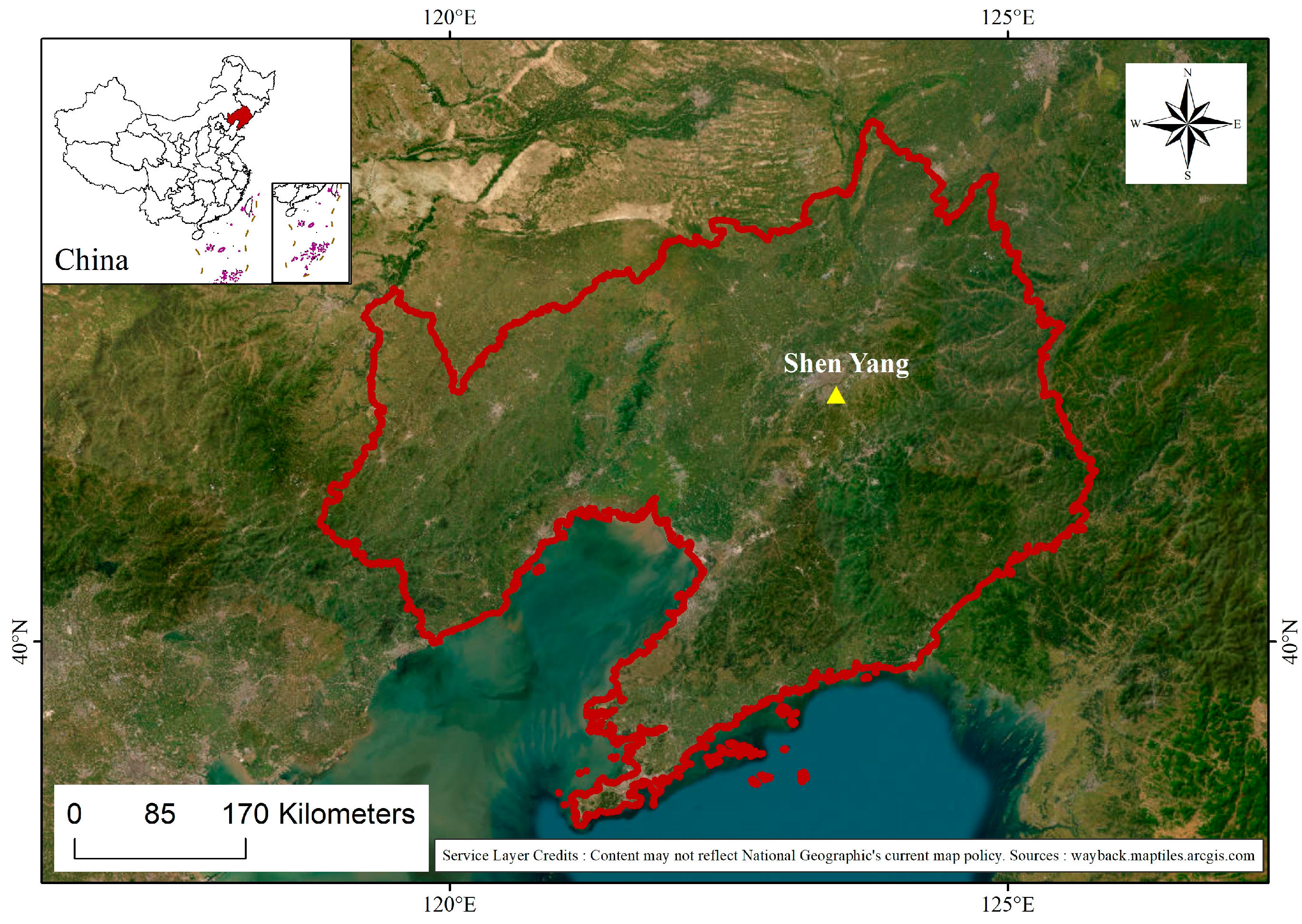
Figure 1.
Overview of the study area. The red region on the inset map shows the location of Liaoning Province in China.

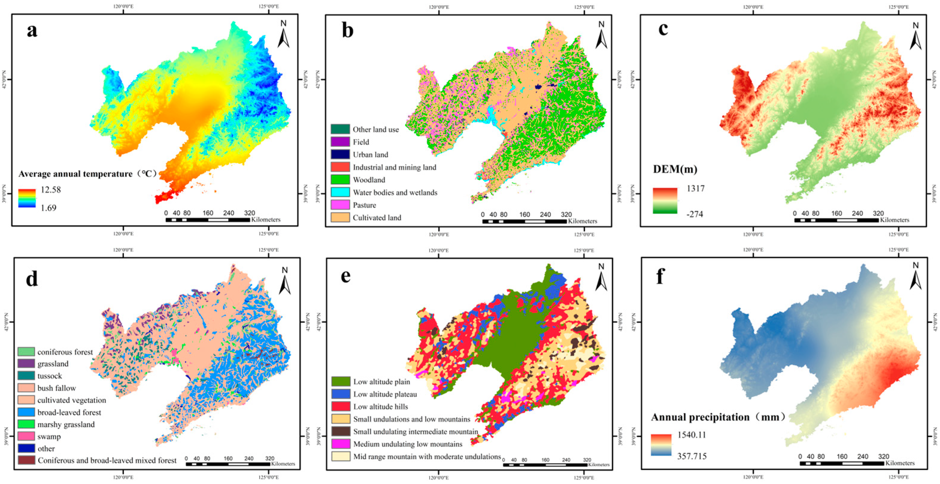
Figure 2.
The environmental variables in the study. Notes, (a): average annual temperature; (b): land use type; (c): vegetation type; (d): vegetation type; (e): geomorphology; (f): annual precipitation.
2.2. Data Acquisition
2.2.1. Data Sources
- (1)
- The sampling data were collected from “Soil series of China—Liaoning Volume” [24] and “China Soil Species (Volume 2)” [25]. A total of 264 data were collected (Figure 3). The sampling period for most soil profiles was during 2008–2020.
 Figure 3. Distribution map of sampling points for collected soil data.
 - (2)
- The environmental variables were average annual temperature, land use type, DEM, vegetation type, geomorphology, and annual precipitation (Figure 2).
The DEM data (meter) in the topographic factors and the 90 m resolution DEM data were obtained from the Geospatial Data Cloud (http://www.gs−cloud.cn, 2 April 2024), an online platform that provides a wide range of geospatial data. Climate factor data (Average annual temperature and precipitation) were obtained from the Ares Environmental Science Data Platform (http://www.res−dc.cn, 3 April 2024).
2.2.2. Data Processing
- (1)
- The defining characteristic of soil in the black soil region is the existence of a black or dark black humus horizon, typically designated by letter A [2,3]. The thickness directly indicates the soil’s fertility and quality [2]. Therefore, in order to evaluate the HHT, the thickness of horizon A was selected as the measurement standard. Predicting the thickness of horizon A allows for a more precise assessment of the fertility status, providing crucial data support for agricultural production and soil management.
- (2)
- In ArcGIS, the reclassification tool can reclassify various data based on specific rules. Following reclassification, 122 samples were determined. To validate the delineated black soil region and assess its accuracy, 85 samples were randomly selected, while the remaining 37 samples were used as validation points. These validation points were chosen to evaluate the accuracy of the study results through comparative analyses.
2.3. Research Methods
2.3.1. Ordinary Kriging
OK is a statistically based spatial interpolation method that uses data from known sample points to predict attribute values in unknown regions [26].
The steps are as follows:
- (1)
- Calculation the distance and semi-variance: calculate the distance between known points is calculated to obtain the corresponding semi-variance.
- (2)
- Fitting the semi-variance function: a curve is chosen to fit the relationship between semi-variance and distance. This relationship is usually expressed through variational function models, including Gaussian, linear, spherical, damped sine, and exponential models.
- (3)
- Determine the range: a range is a specific distance within which attribute values are spatially correlated. Beyond this distance, the attribute values are no longer correlated.
- (4)
- Calculation of weights: for an unknown point, its distance from a known point within the variation is calculated and the semi-variance of the response is derived, which in turn back-calculates the weights (λ).
- (5)
- Performing interpolation: Using the weights (λ) and the attribute values of the known points, the attribute values of the unknown points are calculated by a linear unbiased and optimal estimation method. The formula is as follows.
2.3.2. Inverse Distance Weight Interpolation
IDW is a spatial analysis method based on point data, which uses distance and weight to calculate the value of unknown position [27].
The IDW formula is as follows:
where Z(x0) is the estimated value of position x0, Zi is the value of the ith known sample point, and λi is the weight of the ith known sample point. The weight λi is defined as:
where di0 is the distance between x0 and the ith known sample point, while p is the power parameter to control the influence of distance. A larger value of p makes the influence of closer points stronger and vice versa. n is the total number of known sample points.
2.3.3. Regression Kriging Interpolation
RK is an advanced spatial interpolation method that combines regression analysis and ordinary kriging interpolation [28]. The steps are as follows:
- (1)
- Constructing regression model: Sample data and factors (Vegetation type, Land use type, Average annual temperature, Annual precipitation, DEM (m), and Geomorphology) were used to construct regression model, and extract the main trend of data.
- (2)
- Calculation residuals: Following the construction of the regression model, residuals are computed for each sample point. These residuals represent the discrepancies between the observed values and the predicted values derived from the regression model.
- (3)
- Ordinary kriging interpolation: The calculated residuals are interpolated using the ordinary kriging method to ensure the spatial correlation of the data is fully incorporated.
- (4)
- Combining trend terms and residuals: The final spatial interpolation results are obtained by integrating the trend terms derived from the regression model and the findings from the ordinary kriging interpolation analysis of the residuals.
- (5)
- A multiple regression model was used to fit the HHT distribution map to visualize the interpolation results and their spatial distribution.
The formula is as follows:
where Y represents the actual HHT at the site, β0 is the constant term, and β1, β2, and β3 are the estimated coefficients of the variables x1, x2, and x3, respectively. The final predicted value is given by:
where y(pi) represents the precipitation value at spatial location Pi; βj,(pi) are the coefficients of the regression model; Xj,(pi) denotes the jth independent variable at location pi; ε(pi) is the residual of the regression model, and n is the number of covariates, which in this case is three.
2.3.4. Random Forest Model
The Random Forest Model operate by training numerous independent decision trees, where each tree is built using a distinct subset of data and features [29]. These decision trees undergo a voting process to produce the ultimate prediction. The element of randomness in the training process gives Random Forest a strong resistance to fitting, making it perform well when dealing with datasets with a large number of features and high dimensionality (Figure 4) [30].

Figure 4.
Random Forest principal schematic [30].
The random forest model was trained with a ratio of 0.8, utilizing 100 decision trees. The node splitting criterion was based on squared-error, with a minimum sample number of 2, and an unlimited maximum depth of the tree. The Random Forest algorithm was employed to construct a prediction model, using HHT as the dependent variable and the potentially major influencing factors (vegetation, land use type, mean temperature, annual precipitation, DEM, and geomorphological type) as independent variables, to provide an in-depth exploration of the environmental variables contributing to HHT.
2.3.5. Model Performance Assessment
To evaluate the prediction model’s accuracy, four error metrics were used in this study: ME, MAE, RMSE, RRMSE [30,31].
ME is an indicator used to evaluate the accuracy of a prediction model. It calculates the average value of the difference between the predicted value and the actual value. The average error provides information about the direction and magnitude of the prediction deviation, and the calculation formula is as follows:
ME:
MAE is a measure used to evaluate the prediction accuracy of a model. It calculates the average of the absolute values of the differences between all predicted values and their corresponding actual values. The formula for calculating MAE is as follows:
RMSE is a commonly used metric to measure the prediction error of a model. It is obtained by calculating the square root of the average of the squared differences between the predicted values and the actual values. In statistics, RMSE is widely used in regression analysis and provides a measure of prediction accuracy. The formula for calculating RMSE is:
RRMSE is a metric used to evaluate the prediction accuracy of a model. It is calculated by standardizing the RMSE with the actual range of the observed values. This results in a dimensionless ratio, which facilitates comparison between different datasets or models. The formula for calculating RRMSE is as follows:
where: n represents the number of sampling points in the verification data subset; Zoi and Zpi represent the measured values and predicted values of the sampling points, respectively.
2.3.6. Cross Validation
Cross-validation is a statistical technique used to assess and enhance the efficacy of predictive models. This method evaluates a model’s predictive capability by partitioning the data into distinct, non-overlapping subsets—one designated for training and another for validation. The primary objective of cross-validation is to obtain a more consistent and precise estimation of model performance, thereby mitigating variations in evaluation outcomes due to disparate data splits [30,31].
In the present study, the dataset was randomly divided into a training set and a test set, adhering to a specific ratio (70% for training and 30% for testing), using straightforward cross-validation. Evaluation metrics are derived directly from the test set. If Etest represents an evaluation metric on the test set, then:
2.3.7. Data Histogram
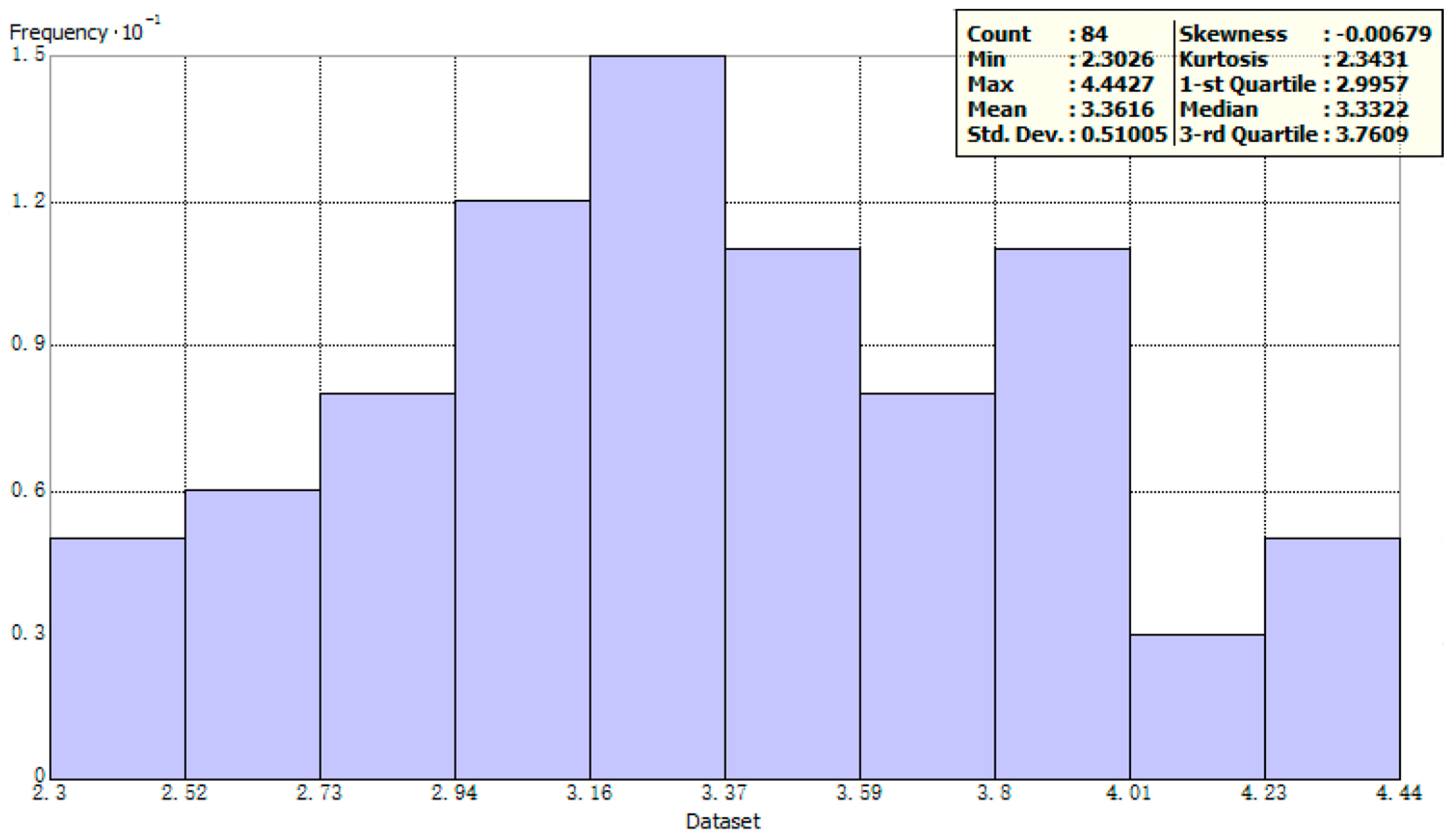
Histograms were constructed after processing the HHT data using Log transformation in ArcGIS 10.7 [21,28].
The difference between the mean and the median is an important indicator of whether the data follows a normal distribution. When the two are close or equal, the data usually show symmetry, suggesting that the data may obey a normal distribution. Kurtosis and skewness are two statistics that describe the distribution pattern of data. The skewness reflects the symmetry of the data distribution. If the data are symmetrical, the skewness is zero, indicating that the data distribution is similar to the normal distribution. If the skewness is greater than zero, the data distribution is right-skewed, with the peaks on the left more concentrated than those on the right. If the skewness is less than zero, the data distribution is left-skewed, with the peaks on the right more concentrated than those on the left. Kurtosis describes the steepness and tail thickness of data distribution. A kurtosis value of zero indicates that the data distribution has the same kurtosis as the standard normal distribution. When kurtosis is greater than zero, it is steeper than normal distribution, with more data clustered near the mean and thicker tails. When kurtosis is less than zero, the distribution is smoother than normal distribution, with more dispersed data.
2.3.8. Data Analysis
The Descriptive Statistics and Calculated Variable in SPSS Statistics 26 were used for data statistics. The ArcGIS 10.7 were used for plotting graphs.
3. Results
3.1. Statistical Characteristics of HHT
The mean and median values of HHT are 30.28 cm and 28.00 cm (Table 1), respectively, which are basically equal, showing some symmetry.

Table 1.
The descriptive statistical eigenvalues of the original sample.
The coefficient of Variation (CV) is 0.55 (Table 1). According to the grade of the CV, the HHT belongs to a high degree of variability, indicating that it is easily affected by the changes in the surrounding environment, and the stability is poor.
The skewness is −0.007 (Figure 5), indicating that the peaks of the data tend to be concentrated on the right side. The kurtosis is 2.34, indicating that the overall distribution of the image is more elevated, and the change is steeper compared with the standard normal distribution, which indicates that the distribution of the data has a thicker tail, i.e., there are more extreme values. This phenomenon may be indicative of an uneven distribution, i.e., the HHT varies considerably between different areas.
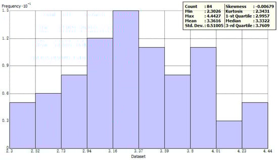
Figure 5.
Histogram of humus horizon thickness data.
3.2. Spatial Distribution Characteristics of HHT
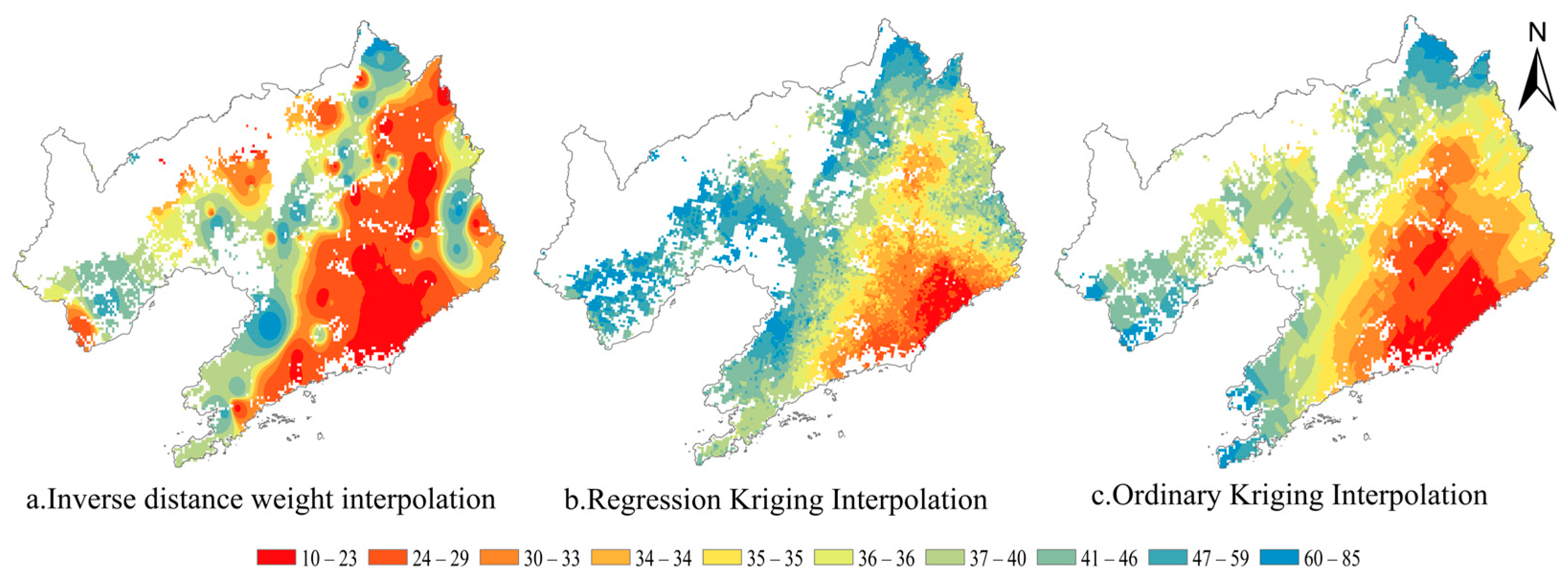
The IDW, RK considering environmental factors, and OK were used to characterize the spatial variation characteristics of HHT (Figure 6). It ranged from 10.20 to 84.55 cm (Figure 6a), 13.12 to 48.60 cm (Figure 6b), and 18.49 to 50.21 cm (Figure 6c), respectively. All results predicted by the three methods show that the HHT changes unevenly, which was consistent with the results showed by Histogram (Figure 5). After in-depth comparative analyses, all three interpolation algorithms can better reflect the distribution characteristics and are consistent with the actual situation.

Figure 6.
Interpolation results for humus horizon thickness.
Comparing and analyzing the predicted results with the actual HHT, it was observed that the results obtained by the IDW best matched the range of fluctuations in the actual observed values. However, the spatial distribution map generated by the IDW lacked smoothness (Figure 6a), which reduced the quality of its visualization. Especially in the region of high values and the dense area of interpolated points, it was easy to appear obvious “bull’s-eye” effect, i.e., the distribution pattern of surrounding high values around a low value point. On the other hand, the OK suffered from the same problem of poor transition smoothness (Figure 6c). Although the RK showed some deviation from the actual soil thickness (Figure 6b), the results showed a higher degree of smoothness and provided a better visualization.
3.3. Suitability Evaluation of Different Interpolation Methods
Soil samples (n = 264) were collected and distributed in various areas, but not all areas were belonged to black soils. After re-classification, 122 samples were screened out. The prediction results were independently validated against the HHT at the validation site to derive the errors (Table 2). Comparing and analyzing the three different interpolation methods, the RK has the smallest ME (11.45 cm), RMSE (14.98 cm), MAE (11.45 cm), and RRMSE (0.44 cm). Conversely, the IDW displayed the lowest accuracy, with corresponding error metrics of 13.81 cm, 18.08 cm, 13.81 cm, and 0.56 cm, respectively, indicating a significant disadvantage. This indicated that the RK has the least difference between the predicted and actual values and is the best prediction results.
Table 2.
The prediction errors of IDW, OK, and RK results.
3.4. Factors Influencing the Humus Horizon Thickness
Vegetation and Land use type can reflect the land use situation. Average annual temperature and precipitation can reflect the climate state. Geomorphology and DEM determine the distribution and types of soil, and also affect the its formation process.
In a random forest model, the sum of the feature weights is one, which is a key metric to help understand the magnitude of each independent variable’s contribution to the model’s predictive power (Table 3).
Table 3.
The characterizations of weight values of different environmental variables.
According to the distribution of feature weights, the following results were obtained:
- (1)
- The independent variable, mean annual temperature, occupied the largest share in the model at 28.56%, indicating that mean annual temperature had the highest influence and was a key factor in model construction.
- (2)
- The weight of average annual precipitation was 27.38%, indicating that it also had an important influence.
- (3)
- DEM had a weighting of 21.12%, which was smaller than the mean annual temperature and precipitation, and had a relatively small degree of influence in the model.
- (4)
- The proportion of land use types is 12.00%, which has a moderate influence, which means that among the variables considered, it has certain explanatory power to predict the HHT.
- (5)
- The proportion of geomorphology was 5.70%, and the contribution was low. It showed that geomorphic factors were not the main factors.
- (6)
- The proportion of vegetation types was 5.20%, with the lowest contribution. This showed that the change of vegetation type was not the main influencing factor, or its influence was relatively weakened compared with other factors.
The weights of the three features (average annual temperature and precipitation, DEM) together accounted for 77.07%, implying that they were the most important features. Although the remaining three independent variables (land use and vegetation type, geomorphology) were relatively small, indicating that their contribution was not as significant as the first three features. Therefore, the average annual temperature and precipitation, DEM were the key influences, whereas land use and vegetation type, geomorphology, although also contributing, were relatively less influential.
4. Discussion
4.1. Characterizing the Spatial Variability of Humus Horizon Thickness
4.1.1. Selection of Interpolation Methods
The environmental variables include a variety of types, which were specifically classified as vegetation, and land use type, mean temperature and precipitation, DEM, and geomorphology. The presence of complex interactions between the variables brought some complexity. Therefore, in the experimental design, the complexity of environmental factors was fully considered, and as many representative typical profile data from the historical soil survey data were collected as possible. These samples were spatially distributed more evenly to ensure the representativeness and to guarantee the accuracy of the statistical inference. Three interpolation methods were used to characterize the spatial distribution of HHT.
In practice, Kriging interpolation is a geostatistical method based on spatial autocorrelation, which assumes that the data is continuous in space [32,33]. The spatial continuity of experimental data might be weakened by a variety of factors [34]. For example, topographic relief, climatic differences, anthropogenic, and other factors might lead to faults or inhomogeneities in the spatial distribution of data [35]. The topography of Liaoning Province is mainly composed of mountains in the east, Liaohe Plain in the middle and low hills and mountains in the west, while the Bohai Sea coast in the south is a long and narrow coastal plain [36]. In terms of climate, Liaoning Province experienced a gradual decrease in precipitation from the southeast to the northwest. The average annual precipitation in Dalian and other places in the southeast can reach more than 800 mm, while that in Chaoyang and Fuxin in the northwest is only 400–500 mm [36].
It was these diverse and variable environmental conditions that directly led to the uneven spatial distribution of HHT, so the OK had a relatively large errors in the results. RK combining environmental variables employed a variability function to describe the spatial variability between data points. By optimizing the variational function model, the spatial structure could be better captured, thus reducing the interpolation error. IDW focused on spatial distance and might ignore other factors [37], such as topography, climate, and human activities. Therefore, IDW was a poor choice when experimental data were affected by multiple environmental variables, while RK, which took into account the topographic complexity, climatic diversity, and human activities, was a more accurate method for predicting the spatial distribution of HHT.
4.1.2. Accuracy of Interpolation Methods
Combined with the RK of environmental variables, the variation function is used, which is the core of kriging interpolation and describes the spatial variability between data points [38]. By optimizing the variogram model, the spatial structure of data can be better captured, thus reducing the interpolation error [39]. Combined with the data characteristics, further analyses concluded that the RK combined with environmental variables was the most accurate interpolation method. Although, the RK had great deviation from the actual, the resulting spatial distribution maps showed high smoothness and provide better visualization effect [40]. This was because the RK not only considered the spatial correlation between sample points, but also combined the influence of environmental variables, so as to better presented the spatial distribution characteristics of the HHT. The result is consistent with the study of effective soil thickness distribution characteristics of arable land obtained by Liu et al. [41].
IDW is a distance-based interpolation method, which is suitable for data sets with strong spatial autocorrelation [42]. IDW interpolation mainly focuses on spatial distance, and ignore other factors that affect the HHT [43], such as topography, climate, and human activities. Although the IDW performed well in reflecting the range of fluctuations in actual observations (Figure 5), it suffered from a lack of smoothing, especially in areas of high values and in areas with a high density of interpolated points, where the “bull’s-eye” effect was likely to be evident [44]. This may be due to the fact that the IDW mainly relied on the imputation of the distance between the sample points, and gave a larger weight that were closer together. It led to the interpolation results being more affected by the local data, thus reducing the smoothness of the spatial distribution maps. This may affect the thickness distribution of humus horizon in black soils [45]. This result is consistent with the results obtained by the interpolation method of equal factors for the quality score of arable land studied by Yang et al. [46].
For the OK, when considering the spatial correlation between the sample points, the same weight was given with different distances, which led to the interpolation results being too smooth and could not well reflect the local change characteristics of the actual observations [47]. It has been demonstrated that the difference between the maximum and minimum values of the numerical result valuation is significantly smaller than the original data. This indicates that the OK has the characteristic of centralizing the distribution of interpolation results, leading to prediction results that are biased towards a larger error, which is also reflected in the present study [48].
In terms of error indicators (Table 3), the RK combined with environmental variables was superior to OK and IDW in ME, RMSE, MAE, and RRMSE. The results were consistent with previous research [49]. However, the IDW had the worst performance on these indicators, which was consistent with the findings of previous studies [50]. RK combined with spatial autocorrelation and the influence of environmental variables made up for the shortcomings of OK and IDW, and improved the interpolation accuracy [51]. Environmental variables, such as DEM, mean annual temperature and precipitation had important effects on spatial distribution [52]. Incorporating these variables into the model combined the strengths of geographic information and statistical modelling to produce smoother maps with lower errors and the highest prediction accuracy when dealing with the problem.
In conclusion, the RK combining environmental variables was the most accurate interpolation method due to its low error indicator performance and intuitive theoretical basis. The method had important practical value in practical application, especially in the fields of environmental science and geographic information system.
4.2. Characterization Results of Spatial Variability of Humus Horizon Thickness
The random forest model was used to analyze the effects of multiple environmental variables, identifying DEM, mean annual temperature and precipitation as key influences driving spatial variability of HHT. A more accurate spatial variability map was produced. It is as follows (Figure 7):

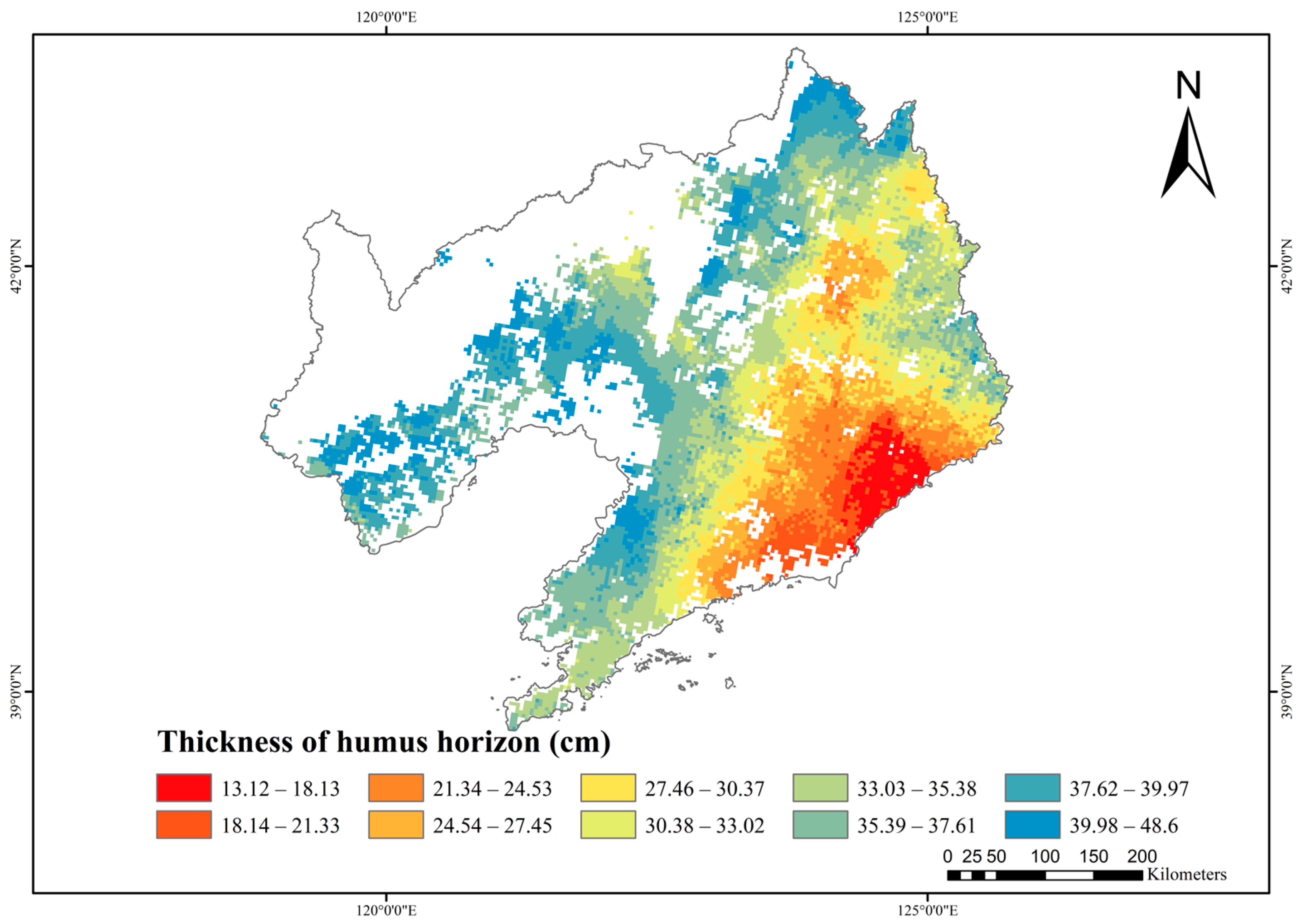
Figure 7.
RK results of humus horizon thickness.
4.2.1. Characteristics of Spatial Distribution of Humus Horizon Thickness
The HHT in Liaoning province is uniform, which is consistent with the result in Figure 5. The HHT increases from the southeast towards the middle and north. The southeast region was the thinnest. However, the northeast and southwest regions exhibit relatively thicker horizons. Along the southern Bohai Sea coast, it is thick but not densely distributed. Chaoyang and Fuxin, located in the northwestern direction, are areas with thick humus horizons, but their distribution is relatively sporadic. Meanwhile, in the northeast direction, Tieling and other locations have thick humus horizons and are aggregated in distribution, albeit covering a relatively small area (Figure 7).
In the southeastern part, it was the thinnest, ranging from about 10 to 20 cm. Climatic factors were one of the important natural factors affecting it [53]. The humid climate and high precipitation with combination of agricultural land use produced strong water erosion, which took away the organic matter and nutrients from the soil, resulting in a decrease of soil thickness and a reduction in soil fertility [54]. In addition, the high humidity environment in the southeastern region enhanced the activity of soil microorganisms [55]. Although soil microorganisms were essential for the decomposition of organic matter and nutrient cycling, excessive microbial activity might also lead to excessive mineralization and decomposition, which accelerated organic matter depletion and affected soil fertility and structural stability [56]. Therefore, in this area, it was relatively thin.
The northeastern region, including the cities of Tieling and Fushun, is located in the upper reaches of the Liaohe River. The river flooding carried a large amount of sediment deposited on both sides of the riverbanks, providing a rich soil-forming parent material [57]. These deposits, which were rich in minerals and other nutrients, were the basis for the formation of fertile soil [2,57]. Tieling and other areas are located in the upper reaches of the Liaohe River, and the special geographical environment makes the river flow moderately, which is conducive to the deposition of alluvial sediments. In addition, many flood events in history had provided a large number of alluvial parent materials, which was an important material basis for the formation of black soil [57].
The northeastern part belongs to temperate continental monsoon climate, which is beneficial to the accumulation of organic matter and the formation of soil clay, thus promoting the development of humus horizon [58]. In addition, the natural vegetation is very lush. Dense forest can not only strengthen the soil through roots, but also provide rich organic matter for the soil under the forest, which is conducive to increasing soil fertility and improving soil structure [59]. Good forest cover also helps to maintain soil moisture, reduce evaporation losses, and regulate surface temperatures, providing a suitable environment for soil organisms, which in turn improves the overall quality and continued productivity of the soil [60].
The western part and the central-western Bohai Sea Rim belt, belonging to the northern temperate continental climate zone and the low mountainous and hilly areas respectively. These areas are subject to frequent invasions of warm air masses coming from the south and the dry-cold air from the Inner Mongolian Plateau, forming a semi-dry, semi-moist and prone-to-drying climatic feature [61]. Winters are cold and dry and summers are hot and rainy. The semi-dry and semi-humid climate is conducive to the growth of vegetation and the accumulation of organic matter. In the wet season, plants grow vigorously, which provides a rich source of organic matter. In the dry season, microbial activity is weakened and the decomposition rate of organic matter slowed down, contributing to the accumulation of organic matter. Moderate precipitation that does not lead to severe soil erosion due to excessive precipitation as in the southeast. Good vegetation coverage on the surface also plays an important role. Plants can prevent soil erosion by fixing the soil through their root systems, but the deadfall of vegetation can increase soil organic matter and improve soil fertility. Vegetation also intercepted precipitation and slowed the impact of rainfall on the soil surface, further protecting the soil structure. The alternating changes in low winter temperatures and high summer temperatures caused cyclical fluctuations in soil temperatures, which promotes the humification process of plant residues, increased the content of soil organic matter and created favorable conditions for the development of black soils [57,58,59].
4.2.2. Variability in the Spatial Distribution of Humus Horizon Thickness
The CV is an important statistical parameter in the in-depth analysis and assessment of soil properties, quantifying the degree of dispersion of values in a dataset [60,61], thus providing a measurement standard [61].
The detailed analysis of the CV revealed that the HHT showed high variability, typically indicating the significant variability. This difference might be caused by many factors, including the difference of natural conditions (such as topography, climate, vegetation, etc.) and anthropogenic activities (such as agricultural cultivation, land use change, urbanization expansion, etc.) [59,60,61].
The reason why the HHT shows high variability:
- (1)
- Environmental sensitivities: The humus horizon is highly sensitive to environmental changes and is susceptible to factors such as climate change and topographical differences. When environmental conditions change, soil organisms, microorganisms, enzymes, and other chemical substances are all affected in some way, thus influencing the black soil evolution process [61]. Liaoning Province has a temperate monsoon climate, with relatively high precipitation in the eastern coastal areas under the influence of the sea. The inland areas in the northwest have a gradual decrease in precipitation, and the variability of climate distribution leads to different degrees of erosion of the humus horizon [36,58]. Liaoning has a diverse topography, and as one of the natural geographic elements, it plays an important role in the redistribution of water and organic matter on the surface. Under different topographic conditions, there are significant differences in the migration, accumulation, and loss patterns of water and organic matter, which directly affect the formation and development of soil layers [59]. Liaoning Province has a rich variety of landform types, ranging from the mountainous hills in the east to the Liaohe Plain in the center to the Bohai Coastal Plain in the west, and these different topographic features have a profound impact on the distribution of water and organic matter [36]. In mountainous areas, the large slope and fast surface runoff rate easily lead to soil erosion [36], making it difficult for organic matter to accumulate in the surface layer, thus affecting the development of the humus horizon [36]. In contrast, in plain areas, the flat topography helps the accumulation of water and organic matter in the top layer of soil, which is conducive to the formation of a thicker humus horizon [59]. At the same time, there are also variations in precipitation across different regions. For instance, Dalian in the southeast receives abundant precipitation, while the northwestern region experiences relatively less. This precipitation gradient also influences soil moisture and organic matter content, further intensifying the spatial variability of HHT [6,54].
- (2)
- The soil-forming parent material of Liaoning Province is mainly influenced by its geological structure and rock types, and the soil formation conditions and history of different regions are different [36,60]. Black soils exhibit varying thicknesses across various regions, types, and development stages within the same region, due to differences in soil mineral composition, combination patterns of soil-forming factors, and interaction intensity [62,63]. The formation of soil is significantly influenced by the types of parent materials, which determine the initial material composition and texture of soil. The soil-forming parent materials are complex and diverse, primarily comprising loess, loess-like materials, alluvial deposits, and floodplain deposits [36]. Due to the differences in the type and distribution of these soil-forming materials, the soil properties are unevenly distributed in space. For example, thick humus horizon may be formed in loess and loess-like material sediment areas, while fertile paddy soil may be formed in alluvial areas for good drainage conditions.
- (3)
- Anthropogenic activity: Several anthropogenic factors play different roles leading to significant differences in the spatial distribution of humus thickness [36]. These factors include land-use practices and soil management measures. The Bohai Coast in the south and the plains in the north-central part of Liaoning Province are the main grain production bases. These areas generally adopt more scientific management methods in land use [1,6]. For instance, conservation tillage techniques, such as straw return and no-tillage sowing, are widely promoted in Northeast China. These techniques have effectively slowed down soil erosion and maintained the organic matter content and structural stability of the soil. These conservation tillage techniques reduce direct soil exposure and the impact of weathering. They also help maintain the HHT by increasing soil organic matter and enhancing the soil’s resistance to erosion and self-recovery. In contrast, the southeastern part is predominantly hilly. This results in a fragmented distribution of arable land, uneven implementation of management measures, and difficult management. Long-term agricultural cultivation and irrational land management practices have significantly impacted the humus horizon. Excessive ploughing, fertilizer use, and single crop planting patterns have damaged the soil structure and accelerated the decomposition of soil organic matter. This has led to the gradual thinning of the humus horizon. Furthermore, with the advancement of urbanization in southeastern part, arable land has been heavily used for industrial and residential construction. This not only reduces the area of arable land but also further destroys the soil structure through construction activities. The changes in land use have directly affected soil protection and recovery mechanisms, making it more difficult to maintain the originally weak humus horizon. Industrial emissions and improper treatment of wastewater may potentially lead to soil pollution, affecting the quality and fertility of the humus horizon.
The high spatial variability indicates the low stability of the humus horizon. This lack of stability may adversely affect the growth of crops, which require stable and fertile soils to ensure optimal growing conditions. It also implies that special attention must be given to soil protection measures in land management and planning to reduce the negative impact of environmental changes on the HHT and to ensure the sustainable use of soil resources.
5. Conclusions
- (1)
- In the study of predicting the spatial distribution of humus horizon thickness, the regression kriging generates relatively smooth images with good visualization and shows a significant advantage over other methods in terms of accuracy. Ordinary Kring may not be able to reach the accuracy level of regression kriging without introducing additional environmental variables. Inverse distance weight interpolation is too simple and relies only on the weights of distances, resulting in its inability to accurately reflect the actual situation in some cases.
- (2)
- The humus horizon thickness fluctuates greatly in spatial distribution and is easily affected by the changes of surrounding environment. Among the six environmental variables selected for this study, mean annual temperature, mean annual precipitation, and DEM are key influencing factors (with a contribution sum of 77.07%) of the humus horizon thickness.
- (3)
- The thickness of the humus horizon in Liaoning Province exhibits an increasing trend from the southeast towards the central and northern directions, with the thinnest horizons found in the southeast. Conversely, the northeast and southwest regions have relatively thicker horizons. Along the Bohai Sea in the south, the humus horizon is thicker but not densely distributed. Chaoyang and Fuxin, located in the northwestern direction, belong to the area with thicker humus horizons, although the distribution of black soil is scattered. Meanwhile, places such as Tieling in the northeastern direction have thick humus horizons and exhibit an aggregated distribution, albeit covering a relatively small area.
Author Contributions
Conceptualization Y.-Y.J. and Z.-X.S.; methodology, Y.-Y.J., Z.-X.S., and J.-Y.T.; software, Y.-Y.J., and J.-Y.T.; validation, Z.-X.S., Y.-Y.J., and J.-Y.T.; formal analysis, Y.-Y.J. and Z.-X.S.; investigation, Y.-Y.J., Z.-X.S., and J.-Y.T.; re-sources, Z.-X.S. and Y.-Y.J.; data curation, Z.-X.S.; writing—original draft preparation, Y.-Y.J., J.-Y.T., and Z.-X.S.; writing—review and editing, Z.-X.S., Y.-Y.J., and J.-Y.T.; visualization, Z.-X.S. and Y.-Y.J.; supervision, Z.-X.S. and Y.-Y.J.; project administration, Y.-Y.J. and Z.-X.S.; funding acquisition, Z.-X.S. and Y.-Y.J. All authors have read and agreed to the published version of the manuscript.
Funding
This research was funded by Applied Basic Research Program of Liaoning Province grant number 2022JH2/101300167; Shenyang Institute of Technology Doctoral Research Initiation Fund Project for Science and Education Integration, grant number BS202302; National Natural Science Foundation of China, grant number 42277285; “Xing Liao Talent Plan” Youth Top Talent Support Program (XLYC2203085).
Data Availability Statement
The original contributions presented in the study are included in the article, further inquiries can be directed to the corresponding author.
Acknowledgments
The authors sincerely thank all the students and staff who provided input to this study. Our acknowledgements also extend to the anonymous reviewers for their constructive reviews of the manuscript.
Conflicts of Interest
The authors declare no conflicts of interest. The funders had no role in the design of the study; in the collection, analyses, or interpretation of data; in the writing of the manuscript, or in the decision to publish the results.
List of Acronyms
| Acronym | Definition |
| HHT | humus horizon thickness |
| OK | ordinary kriging interpolation |
| IDW | inverse distance weighted interpolation |
| RK | regression kriging interpolation |
| ME | mean error |
| MAE | mean absolute error |
| RMSE | root mean square error |
| RRMSE | relative root mean square error |
| DEM | digital elevation model |
| CV | coefficient of variation |
References
- Han, X.Z.; Zou, W.X. Effects and suggestions of black soil protection and soil fertility increase in Northeast China. Bull. Chin. Acad. Sci. 2018, 33, 206–212. [Google Scholar]
- Gong, Z.T.; Zhang, G.L. Pedogenesis and Soil Taxonomy; Science Press: Beijing, China, 2007. [Google Scholar]
- IUSS Working Group WRB. World Reference Base for Soil Resources. International Soil Classification System for Naming Soils and Creating Legends for Soil Maps, 4th ed.; International Union of Soil Sciences (IUSS): Vienna, Austria, 2022. [Google Scholar]
- Xie, L.Y.; Ren, L.H.; Shi, L.K.; Du, C.S. Soil and water loss and anti-erosion countermeasures in Chernozem region of Liaoning Province. Bull. Soil Water Conserv. 2005, 25, 92–95. [Google Scholar]
- Lv, Z.X. Exploration of the sustainable use of sloping arable land in black soil erosion areas. Agro Environ. Dev. 1997, 54, 31–32. [Google Scholar]
- Zhang, X.Y.; Liu, X.B. Key issues of mollisols research and soil erosion control strategies in China. Bull. Soil Water Conserv. 2020, 40, 340–344. [Google Scholar]
- Jiang, Y.; Wang, J.; Yang, J.W. Research progress analysis of black soil region cultivated land quality evaluation index by remote sensing. Eng. Surv. Mapp. 2023, 32, 1–13. [Google Scholar]
- Žížala, D.; Juřicová, A.; Zádorová, T.; Zelenková, K.; Minařík, R. Mapping soil degradation using remote sensing data and ancillary data: South-East Moravia, Czech Republic. Eur. J. Remote Sens. 2019, 52 (Suppl. S1), 108–122. [Google Scholar] [CrossRef]
- Drewnik, Z. Properties and classification of heavily eroded post-chernozem soils in Proszowice Plateau (southern Poland). Soil Sci. Annu. 2019, 70, 225–233. [Google Scholar] [CrossRef]
- Meng, K.; Zhang, X.Y. Mechanisms of black soil degradation in the Songnen Plain and its ecological restoration. Chin. J. Soil Sci. 1998, 29, 100–102. [Google Scholar]
- Matecka, P.; Świtoniak, M. Delineation, characteristic and classification of soils containing carbonates in plow horizons within young moraine areas. Soil Sci. Annu. 2020, 71, 23–36. [Google Scholar] [CrossRef]
- Liu, K.; Dai, H.M.; Liu, G.D.; Wei, M.G.; Yang, J.J. Spatial analysis of land use change effect on soil organic carbon stocks in Sanjiang Plain of China between1980 and 2016. Acta Geol. Sin. 2019, 93 (Suppl. S1), 130–131. [Google Scholar] [CrossRef]
- Song, Y.; Liu, K.; Dai, H.; Zhang, Z.; Zhao, J.; Yang, J.J.; Wei, M. Spatio-temporal variation of total N content in farmland soil of Songliao Plain in Northeast China during the past 35 years. Geol. China 2021, 48, 332–333. [Google Scholar]
- Liu, G.D.; Li, L.J.; Dai, H.M.; Xu, J. Change in soil carbon pool in Songliao Plain and its cause analysis. Geophys. Geochem. Explor. 2021, 45, 1109–1120. [Google Scholar]
- Bu, C.; Cai, Q.; Zhang, X.; Ma, L. Review on development characteristics and ecological functions of soil crust. Prog. Geogr. 2008, 27, 26–31. [Google Scholar]
- Wei, D.; Kuang, E.; Chi, F.; Zhang, J.; Guo, W. Status and protection strategy of Black soil resources in Northeast China. Heilongjiang Agric. Sci. 2016, 1, 158–161. [Google Scholar]
- Han, X.; Li, N. Research Progress of Black Soil in Northeast China. Sci. Geogr. Sin. 2018, 38, 1032–1041. [Google Scholar]
- Taylor, A.; Blum, J.D. Soil age and silicate weathering rates deter-mined from the chemical evolution of a glacial chronosequence. Geology 1995, 23, 979–982. [Google Scholar] [CrossRef]
- Duan, X.W.; Xie, Y.; Ou, T.; Lu, H. Effects of soil erosion on long-term soil productivity in the black soil region of northeastern China. Catena 2011, 87, 268–275. [Google Scholar] [CrossRef]
- Alexandra, K.; Bullock, D.G. A comparative study of interpolation methods for mapping soil properties. Agron. J. 1999, 91, 393–400. [Google Scholar]
- Yang, S.H.; Zhang, H.T.; Guo, L.; Ren, Y. Spatial interpolation of soil organic matter using regression Kriging and geographically. Chin. J. Appl. Ecol. 2015, 26, 1649–1656. [Google Scholar]
- Xu, Y.L.; Luo, M.L.; Liang, B.Y.; Chang, X.L.; Xiang, W.; Zhang, B. Effects of different DEM spatial interpolation methods on soil erosion simulation: A case study of a typical gully of dry-hot valley based on USPED. Prog. Geogr. 2016, 35, 870–877. [Google Scholar]
- Wang, X.M.; Fan, C.; Gao, B.B.; Ren, Z.P.; Li, F. A spatial random forest interpolation method with semi-variogram. Chin. J. Eco-Agric. 2022, 30, 451–457. [Google Scholar]
- Zhang, G.L.; Wang, Q.B.; Han, C.L.; Sun, F.J.; Sun, Z.X. Soil Series of China-Liaoning Volume; Science Press: Beijing, China, 2020. [Google Scholar]
- Office of National Soil Survey. China Soil Species; China Agricultural Publishing House: Beijing, China, 1994; Volume 2. [Google Scholar]
- Jing, S.C. Debris Flow Prediction Model Based on Bayes Discriminant Analysis in Sichuan Province; University of Electronic Science and Technology of China: Chengdu, China, 2013. [Google Scholar]
- Mueller, T.G.; Dhanikonda, S.R.K.; Pusuluri, N.B.; Karathanasis, A.D.; Mathias, K.K.; Mijatovic, B.; Sears, B.G. Optimizing inverse distance weighted interpolation with cross-validation. Soil Sci.. 2005, 170, 504–515. [Google Scholar] [CrossRef]
- Knotters, M.; Brus, D.J.; Voshaar, J. A comparison of kriging, co-kriging and kriging combined with regression for spatial interpolation of horizon depth with censored observations. Geoderm 1995, 67, 227–246. [Google Scholar] [CrossRef]
- Liess, M.; Hitziger, M.; Huwe, B. The Sloping Mire Soil-Landscape of Southern Ecuador: Influence of Predictor Resolution and Model Tuning on Random Forest Predictions. Appl. Environ. Soil Sci. 2014, 2014, 57–66. [Google Scholar] [CrossRef]
- Castro-Franco, M.; Costa, J.L.; Peralta, N.; Aparicio, V. Prediction of Soil Properties at Farm Scale Using a Model-Based Soil Sampling Scheme and Random Forest. Soil Sci. 2015, 180, 74–85. [Google Scholar] [CrossRef]
- Yang, Y.Q.; Yang, L.A.; Ren, L.; Li, C.L.; Zhu, Q.E.; Wang, T.T.; Li, X.R. Prediction for spatial distribution of soil organic matter based on random forest model in cultivated area. Acta Agric. Zhejiangensis 2018, 30, 1211–1217. [Google Scholar]
- Zhang, Z.Q.; Yu, F.Z. Study on the Application of Soil Type Information in Spatial Prediction of Soil Organic Carbon. Chin. Agric. Sci. Bull. 2013, 29, 139–144. [Google Scholar]
- Jin, L.; Heap, A.D.; Potter, A.; Daniell, J.J. Application of machine learning methods to spatial interpolation of environmental variables. Environ. Model. Softw 2011, 26, 1647–1659. [Google Scholar]
- Wu, T. Remote Sensing Characterization of Soil Erosion Intensity and Its Impact on the Spatial Pattern of Cropland Carbon Sequestration Potential in the Degraded Black Soil Region; Jilin University: Changchun, China, 2024. [Google Scholar]
- Gao, F.J.; Ma, Q.L.; Han, W.W.; Shan, P.M.; Zhou, J.; Zhang, S.L.; Zhang, Z.M.; Wang, H.Y. Spatial Variability and Distribution Pattern of Soil Organic Matter in a Mollisol Watershed of China. Environ. Sci. 2016, 37, 1915–1922. [Google Scholar]
- Jia, W.J. Liaoning Soil; Liaoning Science and Technology Press: Shenyang, China, 1992. [Google Scholar]
- Yang, M.X. Evaluating Rainfall Interpolation over the Netherlands; Chang’an University: Xi’an, China, 2015. [Google Scholar]
- Li, Y.; E, S.Z.; Zhao, T.X.; Yuan, J.H.; Liu, Y.N.; Lu, G.B.; Zhang, P. Research Progress on Digital Soil Mapping Methods. Chin. Agric. Sci. Bull. 2024, 40, 146–153. [Google Scholar] [CrossRef]
- Lu, H.L. Comparison of Digital Soil Mapping Methods Based on Feature Selection and Different Machine Learning; Anhui University of Science and Technology: Huainan, China, 2020. [Google Scholar]
- Sun, F.J.; Lei, Q.L.; Liu, Y.; Li, F.L.; Wang, Q.B. Research progress and prospect of digital soil mapping technology. Chin. J. Soil Sci. 2011, 1502–1507. [Google Scholar]
- Liu, Y.J.; Wu, H.Q.; Li, R.; Hao, J.D.; Zhu, L. Study on the Distribution Characteristics of Effective Soil Thickness of Cultivated Land in Tacheng City Based on GIS. Geopatial Inf. 2023, 21, 58–62. [Google Scholar]
- Zhao, J.J.; Zhang, H.Y.; Wang, Y.Q.; Qiao, Z.H.; Hou, G.L. Research on the Quality Evaluation of Cultivated Land in Provincial Area Based on AHP and GIS: A Case Study in Jilin Province. Chin. J. Soil Sci. 2012, 70–75. [Google Scholar]
- Bao, G.J.; Ji, C.; Hou, D.W.; Li, Z.F.; Deng, A.P. Source Apportionment and Response to Landscape Pattern of Health Risk of Cultivated Soil Heavy Metals. Environ. Sci. 2024, 45, 4780–4790. [Google Scholar]
- Yuan, L.; Cao, W.J.; Yang, G.X.; Zhang, L.L.; Mu, X.L. Analysis on the Spatial-temporal Evolution of XCO2 in the Three Gorges Reservoir Region Based on OCO-2 Satellite. Spacecr. Recovery Remote Sens. 2022, 43, 141–151. [Google Scholar]
- Li, Z.Y.; Wei, X.H.; Li, B.S.; Guan, G.Z.; Xu, X.Z.; Lei, L. Spatial Distribution of Soil Calcium on Natural Slope of Karst Peak-cluster in Northern Guangdong Province. Bull. Soil Water Conserv. 2016, 36, 62–68. [Google Scholar]
- Yang, Y.X.; Guo, Y.P.; Zhang, H.; Zhang, L.H.; Sang, J. Interpolation Method of Arable Land Quality Grading Based on Barrier Factors. Trans. Chin. Soc. Agric. Mach. 2019, 50, 157–165+175. [Google Scholar]
- Xie, M.Y.; Wang, Y.; Kang, Y.; Wu, Z.T.; Chen, L.Q.; Liu, Q.; Wu, C.Y.; Zhang, J.M. Study of Spatial Predicting in Soil Attributes Based on Interpolations by Artificial Neural Net-work and Ordinary Kriging. J. Ecol. Rural. Environ. 2021, 37, 934–942. [Google Scholar]
- Zhang, C.R. Study on Chestnut Soil Tier Thickness Model in the Typical Grassland; Inner Mongolia Agricultural University: Hohhot, China, 2008. [Google Scholar]
- Guo, J.H.; Liu, F.; Xu, S.X.; Gao, L.L.; Zhao, Z.D.; Hu, W.Y.; Yu, D.S.; Zhao, Y.G. Comparison of digital mapping methods for the thickness of black soil layer of cultivated land in typical black soil area of Songnen Plain. J. Geo-Inf. Sci. 2024, 26, 1452–1468. [Google Scholar]
- Liu, R.X.; Wang, Z.Q.; Tan, Y.P. The thickness of black soil layer and its influencing factors in a small watershed of typical black soil region in Northeast China. J. Soil Water Conserv. 2024, 38, 346–353, 361. [Google Scholar]
- Liu, K.; Wei, M.H.; Dai, H.M.; Liu, G.D.; Jia, S.H.; Song, Y.H. Spatiotemporal Variation of Black Soil Layer Thickness in Black Soil Region of Northest China. Geol. Resour. 2022, 31, 434–442. [Google Scholar]
- Zhang, X.R.; Jiao, J.Y. Formation and evolution of black soil. J. Jilin Univ. 2020, 50, 553–568. [Google Scholar]
- Chen, Z.Z.; Liu, Y.H. Causes and Hazards of Soil Erosion in the Black Soil Area of Bin County and Measures for its Prevention and Control. Heilongjiang Sci. Technol. Water Conserv. 2009, 4, 240–241. [Google Scholar]
- Meng, X.Z.; Liu, T.; Wang, J.H. A Review of Soil Erosion Research in China’s Black Soil Area. China Rural. Water Hydropower 2010, 10, 36–41. [Google Scholar]
- Zhang, Z.Q.; Cai, H.W.; Zhang, P.P.; Wang, Z.L.; Li, T.T. A GEE-based study on the temporal and spatial variations in the carbon source/sink function of vegetation in the Three-River Headwaters region. Remote Sens. Nat. Resour. 2023, 35, 231–242. [Google Scholar]
- Miao, C.Y.; He, T.H.; Yuan, J.J.; Liu, D.Y.; Yao, R.J.; Ding, W.X. Effects of partial substitution of chemical fertilizer with organic fertilizer on soil organic carbon and sunflower yield in Hetao Irrigation Area. J. North. Agric. 2024, 52, 46–54. [Google Scholar]
- Gao, Y. Study on the Distribution Characteristics of the Composition and Properties of Black Soil Humus with Two Parent Materials; Jilin Agricultural University: Changchun, China, 2019. [Google Scholar]
- Wang, Z.Y.; Fu, Y.R.; Zou, B.Z.; Su, X.P.; Wang, S.R.; Wan, X.H. Dynamics Study on Soil and the Characteristics of Under story Vegetation Under Different Restoration Modes in Subtropical Forests. Fujian Agric. Sci. Technol. 2021, 52, 7–16. [Google Scholar]
- Li, J.; Liu, Y.R.; He, J.Z.; Zheng, Y.M. Insights into the responses of soil microbial community to the environmental disturbances. Acta Sci. Circumstantiae 2013, 33, 959–967. [Google Scholar]
- Pan, Y.; Peng, H.; Xie, S.; Zeng, M.; Huang, C. Eight Elements in Soils from a Typical Light Industrial City, China: Spatial Distribution, Ecological Assessment, and the Source Apportionment. Int. J. Environ. Res. Public Health 2019, 16, 2591. [Google Scholar] [CrossRef]
- Usowicz, B.; Lipiec, J. Spatial variability of saturated hydraulic conductivity and its links with other soil properties at the regional scale. Sci. Rep. 2021, 11, 8293. [Google Scholar] [CrossRef]
- Suleymanov, A.; Komissarov, M.; Asylbaev, L.; Khasanov, A.; Khabirov, L.; Suleymanov, R.; Gabbasova, L.; Belan, L.; Tuktarova, L. Spatial Variations of Genetic Horizons Thicknesses and Erosion Degree Assessment in Temperate Soils. Environ. Process. 2024, 11, 44. [Google Scholar] [CrossRef]
- Li, R.; Hu, W.; Jia, Z.; Liu, H.; Zhang, C.; Huang, B.; Yang, S.; Zhao, Y.; Zhao, Y.; Shula, M.K.; et al. Soil degradation: A global threat to sustainable use of black soils. Pedosphere 2024, 2010, 87–97. [Google Scholar] [CrossRef]


Disclaimer/Publisher’s Note: The statements, opinions and data contained in all publications are solely those of the individual author(s) and contributor(s) and not of MDPI and/or the editor(s). MDPI and/or the editor(s) disclaim responsibility for any injury to people or property resulting from any ideas, methods, instructions or products referred to in the content. |
© 2024 by the authors. Licensee MDPI, Basel, Switzerland. This article is an open access article distributed under the terms and conditions of the Creative Commons Attribution (CC BY) license (https://creativecommons.org/licenses/by/4.0/).