Simulating Soil Moisture Dynamics in a Diversified Cropping System Under Heterogeneous Soil Conditions

Abstract

Agro-ecosystem models are useful tools to assess crop diversification strategies or management adaptations to within-field heterogeneities, but require proper simulation of soil water dynamics, which are crucial for crop growth. To simulate these, the model requires soil hydraulic parameter inputs which are often derived using pedotransfer functions (PTFs). Various PTFs are available and show varying performance; therefore, in this study, we calibrated and validated an agro-ecosystem model using the Hypres PTF and the German Manual of Soil Mapping approach and adjusting bulk density for the top- and subsoil. Experimental data were collected at the “patchCROP” landscape laboratory in Brandenburg, Germany. The daily volumetric soil water content (SWC) at 12 locations and above ground biomass at flowering were used to evaluate model performance. The findings highlight the importance of calibrating agro-ecosystem models for spatially heterogeneous soil conditions not only for crop growth parameters, but also for soil water-related processes—in this case by PTF choice—in order to capture the interplay of top- and especially subsoil heterogeneity, climate, crop management, soil moisture dynamics and crop growth and their variability within a field. The results showed that while the impact of bulk density was rather small, the PTF choice led to differences in simulating SWC and biomass. Employing the Hypres PTF, the model was able to simulate the climate and seasonal crop growth interactions at contrasting soil conditions for soil moisture and biomass reasonably well. The model error in SWC was largest after intense rainfall events for locations with a loamy subsoil texture. The validated model has the potential to be used to study the impact of management practices on soil moisture dynamics under heterogeneous soil and crop conditions.

1. Introduction

Achieving sustainability in agriculture requires innovative cropping systems that promote the delivery of ecosystem services (ESS) and enhance biodiversity, while increasing or maintaining crop productivity [1]. Aiming to increase sustainability, crop diversification has been proposed as one path to transform agricultural systems [2,3]. Additionally, small field arrangements adapted to heterogeneous soil conditions could have benefits in the delivery of ESS and biodiversity [4,5,6,7]. Soil heterogeneities regarding, e.g., soil texture, soil horizon depths, soil organic carbon (SOC) and resulting soil moisture, can lead to small scale variability of crop growth and yield formation [8,9]. With precision farming and digital technologies gaining traction, management (e.g., fertilization, crop allocation) can be adjusted to within-field soil heterogeneities [10]. Nutrient dynamics are highly dependent on soil moisture and soil temperature, as well as the soil’s clay content [11,12]. Managing these spatial differences could lead to improved resource use efficiency in terms of fertilizer input. Since experiments to adjust and improve crop allocation or fertilization to site-specific soil conditions would require substantial effort, agro-ecosystem models could serve as a tool to test the impact of these approaches on crop productivity by capturing crop interactions under heterogeneous soil conditions [13,14,15,16]. Additionally, agro-ecosystem models can be useful tools to assess the combined effect of management and climate on agricultural production, as well as the delivery of ESS and biodiversity [17,18,19,20]. To achieve this, location-specific processes that drive crop growth need to be captured by the models.

As weather patterns are mostly stable within the field, the driving factors for within-field heterogeneity are the soil conditions [21,22], which impact water and nutrient dynamics. Drainage processes in point-based models can be simulated with a relatively simple “tipping-bucket” approach or based on more complex Darcy’s or Richards’ equations that allow a continuous representation of water movement [20]. Models focusing on crop growth simulations (WOFOST, DSSAT, APSIM, STICS, MONICA) often work with conceptual approaches like the tipping-bucket approach to simulate soil water dynamics [23]. It has been debated that the use of conceptual approaches introduces unnecessary empiricism when more physics-based approaches could be used [24]. While there have been studies coupling (physics-based) hydrological and crop models [25], the physics-based models require sub-daily time steps and have higher computational requirements [26]. Following this debate, Vianna et al. tested how soil moisture prediction was affected by the model structure and data detail, and found both the Richards’ equation and tipping-bucket model approach to perform similarly well, with only a slight improvement when using the physics-based model [27]. Additionally, Longo et al. found a tipping-bucket-based approach to be sufficient at deep groundwater tables [28]. Similarly, Soldevilla-Martinez et al. [29] compared the DSSAT model, which incorporates a tipping-bucket approach with the more mechanistic Richard’s equation-based WAVE model, and found that both models performed well for simulating the soil water content, while WAVE showed a better simulation of drainage. To initialize and parametrize soil water balance models, additional information about soil hydraulic properties is needed, which can be challenging to measure in the field for multiple locations. Therefore, pedotransfer functions (PTFs) are commonly used to translate more readily available soil data into soil hydraulic properties [30]. Weihermüller et al. differentiated between continuous, equation-based PTFs, which require soil particle size distribution, organic carbon and bulk density; and class-based PTFs, which are based on, e.g., soil textural class [31]. Various continuous PTFs have been developed, focusing on specific regions to account for similar pedogenetic factors and, consequently, soil conditions [32,33,34], and have shown varying performances [35,36,37]. Rosso et al. tested how the simulation of SWC was impacted by the PTF by employing a tipping-bucket model (HERMES) with six PTFs at four locations in Germany [38]. The results suggested that careful PTF selection is important as the PTF performance was location specific. In Germany, the soil hydraulic properties tabulated in the “Bodenkundliche Kartieranleitung” [39] are the most important and widespread source with which to estimate the soil hydraulic properties from the soil textural class, bulk density and soil organic matter content for each soil layer. One advantage of employing this method is that it does not require cost intensive laboratory analysis of particle size distribution, but rather soil textural class, which can be determined manually in the field [40]. However, very few publications have tested their usefulness and performance to simulate soil water fluxes in process-based simulation models, capture within-field variability of soil moisture and crop growth and compared them to other approaches like continuous pedotransfer functions. Therefore, there is a need to test and compare different estimation approaches. A range of continuous PTFs is available, developed based on datasets from different regions, such as Rawls [41] (US), Rosetta [42] (US and EU), Toth [33] (EU) and Hypres [34] (EU). As this study was conducted in Germany, Toth and Hypres were the most fitting choice, given the databases are from European soils. Weihermüller et al. tested PTF performance and found Hypres and Toth to perform comparably robustly, with a slightly better performance of Hypres for simulating water fluxes [31]. Therefore, in this study, Hypres was chosen to be compared to the BK.

For agro-ecosystem models covering a large range of crops, to be applied reliably and to be able to spatially quantify the interactive effects of climate, soils and management on crop growth, crop productivity and the environment, they need to be tested on their capability to adequately simulate the effects of climate, crop rotation and soil heterogeneities on soil water dynamics. The main goals of this study were to (1) develop and calibrate an agro-ecosystem model which is able to adequately simulate the effect of climate, crop rotations and soil heterogeneity on soil water content within the root zone as well as crop growth; and (2) to identify the most suitable approach to derive soil hydraulic properties as a crucial input to the model by evaluating its impact on the simulation of soil moisture dynamics and biomass production of different crops. We assume that the validated agro-ecosystem model is able to reproduce the interactive effect of climate and seasonal crop development within different crop rotations and heterogeneous soil conditions on site-specific daily soil moisture dynamics and above ground biomass.

2. Materials and Methods

2.1. Location

The landscape laboratory “patchCROP”, established in 2020, comprises an experiment with a 70 ha field in Tempelberg, Brandenburg, in North-East Germany. This area is characterized by young moraine landscapes with heterogeneous soil conditions with a mean annual temperature of 9.2 °C and a mean annual precipitation of 568 mm. Groundwater levels in Tempelberg are about 20 m below the surface and, therefore, well below the plant root zone [43]. To explore the potential of diversified cropping systems that operate at smaller field scales than current farming practice in Eastern Germany and considering spatial differences in soil characteristics, 30 so-called “patches” with a size of 0.52 ha each were established in 2020. The patch size was based on the minimum units that can be managed with current machinery. For patch delineation, Donat et al. used past yield maps of ten years when the 70 ha field was managed homogenously to identify a high and low yield potential zone within the field, with 15 patches allocated to each zone [44]. For the current study, eleven out of the 30 patches were considered (Figure 1a). Six patches were located in the high yield potential (HYP) zone, where the crop rotation consists of rapeseed (Brassica napus L., cv. Ambassador), winter barley (Hordeum vulgare L., cv. Wallace), cover crop, soybean (Glycine max L., cv. Acardia), cover crop, maize (Zea mays L., cv. P8349) and winter wheat (Triticum aestivum L., cv. Universum). The remaining five patches were located in the low yield potential (LYP) zone. Here, sunflower (Helianthus annuus L., cv. Seabird), winter oat (Avena sativa L., cv. Fleuron), cover crop, maize, lupine (Lupinus angustifolius L., cv. Boragine), winter rye (Secale cereale L., cv. Tayo) and a cover crop are grown in rotation.

Weed and pest management in the patches were either managed according to (1) standard farm practices with full herbicide, fungicide and pesticide application; (2) with reduced chemical-synthetic plant protection measures; or (3) with reduced chemical-synthetic plant protection measures and flower strips. Crop management was conducted by the farm adhering to conservation agriculture principles. Crop residues remained on the field and ploughing was omitted. Only for seed bed preparation, a shallow or deep chisel plough from 15 to 25 cm depth was employed. The patches themselves were managed homogenously in regard to sowing and fertilization. Each patch had a buffer zone of 18 m width surrounding the center, which was split into four quadrants (Figure 1b). In each patch, a soil, yield and biodiversity quadrant was dedicated to the respective sample collection. Daily weather data (mean, maximum and minimum temperature, precipitation, solar radiation, wind speed and relative humidity) were obtained from two on-site weather stations.

2.2. Data Collection

2.2.1. Soil Data

Soil sampling at the study site was conducted between 2020 and 2023. The dataset comprises soil information collected at 16 locations along transects within the yield and soil quadrant of the respective patch. Soil augers were taken with a 1 m long Pürckhauer. Once the soil was extracted, soil layers were determined using visual assessment for color differences and manual assessment for density differences. For each layer, the textural class, color, stone content, presence of mottles and CaCO₃ were determined in the field. The soil textural class was assessed manually according to the German soil texture classification method (Fingerprobe zur Bestimmung der Bodenarten in Anlehnung an DIN 19682-2 und KA5, 2012), as described by Vos et al. [40]. The color was evaluated using a wetted and mixed soil sample with the Munsell soil color chart [45]. Stone content (based on visual evaluation), CaCO₃ (droplet application of 10% HCl, visual and sound evaluation for foam presence or effervescence) and mottle presence (visual evaluation) were assessed following the FAO procedure [46].

Up to December 2023, 256 locations were sampled; out of these, 50 locations were resampled to collect soil material for laboratory analysis of particle size distribution (sand, silt and clay content according to DIN ISO 11277 [47] using the SEDIMAT 4-12 (Umwelt-Geräte-Technik GmbH, Müncheberg, Germany)), total organic C and N, pH and extractable P and K. The criteria for resampling were that the location featured reoccurring soil textural classes within a patch or locations where manual soil texture determination was ambiguous. Based on laboratory analysis, the manual readings from the field were adjusted when necessary. Within each yield potential zone, the average particle size distribution of the soil textural classes was calculated (Figure S1) and extrapolated to the respective layers where soil texture was determined manually (

Table 1. Average particle size distribution as percentage of sand, silt and clay by yield potential zone and soil textural class.

	High Yield Potential			Low Yield Potential
Text. Class 1	Sand%	Silt%	Clay%	Sand%	Silt%	Clay%
Ss	86.4	9.8	3.8	91.0	5.9	3.1
Su2	80.9	15.0	4.1	83.4	12.9	3.7
Su3	67.9	26.6	5.5	NA	NA	NA
Sl2	70.8	22.5	6.7	79.7	14.5	5.8
Sl3	66.7	24.0	9.3	72.5	18.0	9.5
Sl4	59.0	25.5	15.5	65.0	20.0	15.0
Ls4	57.7	22.6	19.7	56.5	24.0	19.5

¹ Text. class = soil textural class; Ss = sandy sand, Su2 = slightly silty sand, Su3 = medium silty sand, Sl2 = slightly loamy sand, Sl3 = medium loamy sand, Sl4 = strongly loamy sand, Ls4 = strongly sandy loam.

). For the current study, soil textural class in the last soil layer was assumed to be the same up to 2 m depth.

Bulk density was assessed in two staggered campaigns in March 2021 and 2022. At each patch, five locations were sampled vertically along a transect in the soil quadrant in 4 depth increments (2–7, 11–16, 20–25 and 29–34 cm) by inserting Eijkelkamp steel cylinders. Soil samples were dried for 48 h at 105 °C and stones were removed subsequently by sieving to calculate the stone-corrected bulk density.

2.2.2. Observed Soil Moisture Data

In 2020, soil moisture sensors were installed in the soil quadrant of each patch. The data were recorded using a long-range-wide-area network (LoRaWAN) system, of which one node box (DriBox, Lancashire, UK) was installed at least 30 cm below the ground to avoid interference with tillage. Each node box recorded the volumetric soil water content (SWC) of two locations, where TDR sensors (Acclima TDR310H, Meridian, MS, USA) were installed at 30, 60 and 90 cm depth in angles between 45° and 60°. The distance between the measurement locations was three to five meters. Soil moisture data were recorded every 20 min, transferred to a cloud system via modem and made accessible immediately after measurement. An automated validation process, implemented in the cloud system by the service provider, included data profiling to detect and address errors. Identified anomalies, such as recurring or abrupt erroneous jumps (e.g., a specific value of 28.6% caused by a known sensor manufacturing defect), were removed from the dataset. The measurement accuracy of the sensors, as indicated by the retailer, is ±3 Vol% [48]. Sensor calibration was carried out by the retailer before installation. Data gaps caused by transmission failures, such as battery discharge, signal disturbances, or theft, were minimal due to enhanced maintenance and monitoring efforts. For detailed information on the LoRaWAN soil sensor setup refer to Scholz et al. [49]. For the current study, data from 11 patches were considered, covering the period from 1 January 2021 until 15 September 2022, as a daily average for each TDR sensor. Within this timeframe, approximately 10% of data was missing due to technical problems.

2.2.3. Pairing of Soil Moisture and Soil Textural Data

To evaluate the model’s ability to simulate soil water content, soil auger data and observed soil moisture data were paired, taking spatial proximity and soil heterogeneity into account. This approach aimed to ensure that the selected soil profile, which was later used as basis for model input, accurately represented the soil conditions where soil moisture sensors were located. Generally, the observed soil moisture data at a given location were calculated as the daily average of both soil moisture sensors per depth (30, 60 and 90 cm). In patches where the surrounding soil profile locations showed high heterogeneity in layers and texture, only the soil moisture sensor closest to the paired soil profile was considered (

Table 2. Patch properties and TDR soil moisture sensor information for selected augers at the patchCROP experimental site, located in Tempelberg, Brandenburg.

Patch	Auger Locations Considered 1	Homogeneity of Soil 2	Auger ID	Source of Soil Moisture Data 3	Incorporation of 60 cm TDR Sensor 4	Distance of Auger to Left/Right Sensor [m] 5
12	1	yes	12-s-2-2	average	discarded	2.9/1.5
19	1	no	19-s-2-2	average	considered	3.7/1.6
58	1	yes	58-s-2-2	average	discarded	2.3/2
65	2	no	65-s-2-3	left	considered	2/NA
			65-s-2-2	right	considered	NA/1.6
66	1	no	66-s-1-2	left	considered	0.7/NA
76	2	yes	76-s-1-3	average	considered	3/5
81	2	yes	81-s-2-2	average	discarded	5/1.7
89	2	no	89-s-2-3	right	considered	NA/2
95	2	yes	95-s-2-2	average	discarded	4.6/2.3
102	2	no	102-s-2-3	right	considered	NA/1.8
114	1	yes	114-s-2-2	average	discarded	5.3/2.7

¹ Number of soil augers per patch that were in close proximity to soil moisture locations and where considered when pairing simulated soil moisture at this location and observed soil moisture data; ² considering the four soil auger locations, closest to soil moisture sensors; yes = the soil layers and texture was similar; no = the soil layers or soil texture differed considerably (e.g., appearance of a loamy layer vs. totally sandy soil profile); ³ average = for each depth (30, 60, 90 cm), the average of the right and left TDR sensor of the patch was used; left/right = only data from the TDR sensors in the left or right location were used; ⁴ in cases of soil textural changes at around 60 cm depth, soil moisture data from this depth were discarded; ⁵ NA = TDR sensor was not considered for respective Auger ID.

). In other cases, two soil augers were situated close to both the left and right soil moisture sensor locations. The augers always had a distance of 5 m between them (Figure 1b). If these two augers showed very similar soil properties throughout the 1 m profile, the soil profile of the closest auger point was used and paired with the average as described above. In cases where soil profiles showed distinct differences in soil texture and/or layering, we assumed high soil heterogeneity in this area. Therefore, each profile was matched with the respective closest soil moisture sensors, but only considered when the distance between soil profile and sensor location was less than 2 m, ensuring that observed and simulated moisture data in each soil depth resulted from the same soil textural class. Additionally, the observed moisture data from 60 cm depth were discarded if the soil profile in the paired auger exhibited a change in soil texture close to this depth, to avoid mismatches.

While most of the twelve selected locations were manually assessed for soil texture (

Table 3. Soil layer information for 12 locations within the patchCROP experiment in Tempelberg, Brandenburg, Germany.

High Yield Potential					Low Yield Potential
Patch-ID	Cali./ Vali. 1	Auger ID 2	Bottom Depth (cm)	Textural Class 3	Patch-ID	Cali./ Vali. 1	Auger ID 2	Bottom Depth (cm)	Textural Class 3
12	C	12-s-2-2	33	Sl3	76	C	76-s-1-3	40	Sl2
			45	Sl3				75	Ss
			65	Ls4				100	Ss
			96	Ls4	89	C	89-s-2-3	40	Sl2
19	V	19-s-2-2	43	Su3				70	Sl2
			65	Su3				100	Ss
			87	Su3	95	C	95-s-2-2	38	Su2
			100	Sl4				58	Su2
58	C	58-s-2-2	33	Su3				90	Ss
			44	Su3				100	Ss
			56	Su3	102	V	102-s-2-3	35	Su2
			81	Sl4				87	Ss
			100	Sl4				100	Ss
65	C	65-s-2-2	41	Sl2	114	V	114-s-2-2	39	Ss
			67	Sl2				61	Sl4
			100	Ss				99	Sl4
65	V	65-s-2-3	33	Sl2
			47	Sl2
			58	Sl2
			79	Ss
			100	Sl4
66	C	66-s-1-2	40	Sl2
			58	Sl2
			76	Sl2
			100	Ls4
81	V	81-s-2-2	40	Sl2
			58	Sl3
			100	Ls4

¹ Cali./Vali. = set for calibration (C) or validation (V); ² Auger ID representing (“patchID”–“soil(s) or yield(y) quadrant of the patch”–“transect ID”–“auger ID”; ³ Ls4 = strongly sandy loam, Sl2 = slightly loamy sand, Sl3 = medium loamy sand, Sl4 = strongly loamy sand, Ss = sandy sand, Su2 = slightly silty sand, Su3 = medium silty sand.

) and particle size distribution was therefore extrapolated, as described previously, for one location (12s22) the auger specific particle size distribution was measured in the laboratory.

2.2.4. Crop Management

Table 4. Sowing dates and fertilizer amounts for selected summer and winter crops as applied at the patchCROP site in Tempelberg, Brandenburg, Germany.

Crop	Season	Sowing Dates	Fertilizer Dates	Fertilizer Amount (Total N [kg N ha−1])
Grain maize	2021	16 April 2021	16 April 2021	13.5
			17 April 2021	101.1
			04 June 2021	61.3
	2022	29 April 2022	20 May 2022	71
			23 June 2022	60.7
Soybean	2021	15 May 2021	-	-
	2022	10 May 2022	-	-
Sunflower	2022	31 March 2022	31 March 2022	18.0
			05 April 2022	54.0
Lupine	2022	18 March 2022	-	-
Phacelia	2021	08 September 2021	-	-
Winter wheat	2022	15 November 2021	11 March 2022	80.0
			05 April 2022	44.3
			19 May 2022	55.1
Winter barley	2021	21 September 2020	17 March 2021	48.2
			08 April 2021	71.1
			07 May 2021	25
Winter oats	2021	27 October 2020	17 March 2021	61.5
			08 April 2021	58.7
Winter rye	2021	02 October 2020	17 March 2021	61.5
			01 April 2021	51.1
			14 May 2021	25

provides the crop management data on sowing and nitrogen (N) fertilization dates and rates as carried out by the farm. In 2021 and 2022, the planting of summer crops relevant for this study (maize, soybean, sunflower and lupine) was carried out between mid-March and mid-May, while winter crops (barley, wheat, rye and oats) were sown between end of September and mid-November and the cover crop phacelia was sown at the beginning of September in 2021. Except for lupine, soybean and the cover crop, each crop was N fertilized either two or three times during their growing season. To avoid crop deficiencies, potassium, phosphorus and magnesium fertilizer were applied as needed.

2.2.5. Biomass

The above ground biomass samples were collected after the crop reached the end of flowering (Table S2), representing an adequate time period for the crop biomass to reflect spatial differences. Samples were collected at four georeferenced locations along the edges of the yield quadrant of the respective patch and oven-dried at 60 °C for 48 h to determine the dry weight. The sampled area ranged from 0.5 m² for winter crops to 1.5 m² for maize. Biomass samples were only considered if soil properties of the closest auger location were similar in terms of soil texture and horizon depth to the soil profile used for the simulation and assessment of soil moisture. For patch 102, this led to a discard of biomass data due to inconsistent soil conditions. In the case of patch 66, only the year 2022 was considered for biomass assessment, as the 2021 biomass was collected in areas which were not representative of the soil conditions observed for soil auger 66s12. Additionally, in patches 114, 12 and 89, biomass data of either 2021 or 2022 were not considered in this study as weed pressure was high (>20% total weed cover), which cannot be captured by the model.

2.3. Model Description

The modelling framework Scientific Impact Assessment and Modelling Platform for Advanced Crop and Ecosystem management (SIMPLACE, www.simplace.net (accessed on 19 April 2024)) consists of complementary but interchangeable submodels, called SimComponents, which represent relevant crop- and soil-related processes [50]. A model solution (or agro-ecosystem model) is made up of several SimComponents, which are chosen based on the research question to be addressed and available data. For this study, <Lintul5, SlimWater and SoilCN> as main SimComponents were selected for the model solution. The SimComponent Lintul5 simulates crop phenological development based on temperature sum and, for winter crops, is based on photoperiod, whereas potential crop growth (biomass and grain yield) is simulated based on radiation use efficiency [51]. In this model setup, actual biomass accumulation in the SimComponent Lintul5 is also affected by water and nitrogen limitation using reduction factors TRANRF (transpiration reduction factor) or NNI (nitrogen nutrition index), which range from 0 (full stress) to 1 (no stress). The TRANRF is calculated as a ratio of actual transpiration and potential transpiration. The SimComponent SoilCN, based on a multi-storage pool concept for multi-layered soil profiles [52], was used for simulation of turnover processes regarding soil organic carbon and nitrogen. The model simulates in a daily time step.

2.3.1. Simulated Soil Water Dynamics

The soil water balance was simulated using the SimComponent SlimWater, which uses a tipping-bucket approach where the soil profile is further subdivided into layers of 5 cm (user defined). For each layer, information on certain soil matrix potentials (e.g., saturated, field capacity, wilting point), as well as initial water content, needs to be provided based on the soil conditions at the respective location. The lower boundary condition for simulation was free drainage. The component estimates the daily soil water content of each layer based on water input and outflow (e.g., precipitation, run-off, percolation, soil evaporation, deep seepage). Percolation is calculated vertically starting from the first layer. Water is considered mobile water when the layer’s water content exceeds field capacity. The percentage of mobile water that is routed to the below layer is dependent on the parameter SlimAlfa, which is calculated using the soil layer’s clay content [53]. The simulations are point-based and do not consider lateral water flow. Evapotranspiration was calculated based on the FAO approach by Allen et al. [54] and reference evapotranspiration by Hargreaves using solar radiation and temperature [55].

2.3.2. Pedotransfer Functions and Bulk Density

Two PTFs for deriving soil hydraulic properties were considered in this study. Firstly, we tested the PTF provided in the German manual of soil mapping (Bodenkundliche Kartieranleitung KA5, referred to as BK) [39] (p. 350), which utilizes the German soil textural classes. Hydraulic properties for this method are texture class specific and included field capacity, wilting point and saturation, which are based on matrix potential, 2.5, 4.2 and ∞, respectively. Bulk density was not considered in this approach. Instead, the values were representative of the mean overall bulk density classes, with a mean of 1.5 g/cm³. Secondly, the Hypres PTF [34], implemented as SimComponent in the SIMPLACE framework, was used. The method consists of continuous functions that predict soil hydraulic properties based on a European soil database. They require soil particle size distribution, bulk density and organic matter content by soil layer as input. Since no bulk density data were collected near the auger points, two bulk density setups were chosen based on previous data collection at other locations within each patch (data not published). While absolute values differed, it was apparent that bulk density always increased with increasing soil depth. Based on the previous data collection at various locations within the field, two scenarios were considered reasonable input for the model: (1) a bulk density of 1.3 g/cm³ in the topsoil layer and 1.5 g/cm³ in the subsoil layers, referred to as “Hypres1315”; and (2) a bulk density of 1.5 g/cm³ in the topsoil layer and 1.7 g/cm³ in the following subsoil layers, referred to as “Hypres1517”. Soil hydraulic data based on these three setups (BK, Hypres1315 and Hypres1517) were then used as input for the model solution.

2.3.3. Crop Parameters

SimComponent Lintul5 was used with crop specific parameters for winter barley, soybean, maize, winter wheat, sunflower, lupine and winter rye, which were previously calibrated and validated based on ground-truth intermediate and final biomass cuts and grain yield data using a cross-validation approach [56]. Additionally, the parameters for winter oat and the cover crop Phacelia (Phacelia tanacetifolia Bentham L., cv. Stala) were manually calibrated based on phenology observations and intermediate and final biomass data from 2020 (Table S1). Data for manual calibration of winter oat additionally comprised yield. In the simulation, crops are harvested by default when reaching a developmental stage (DVS) of two, which indicates physiological maturity. However, as phacelia was also sown as a cover crop in autumn and died off during winter, we introduced a termination setting where phacelia is harvested when reaching a DVS of two, or when the daily mean temperature dropped below −7 °C or when the 60th day of year (DOY) was exceeded. The temperature limit of −7 °C was chosen based on available literature and variety-specific information from seed producers [57,58,59].

2.4. Model Initial Conditions

The daily simulations were performed with soil hydraulic property (field capacity, saturation point, wilting point) inputs from each PTF setup (

Table 5. Source and input for each pedotransfer setup used to derive soil hydraulic properties for the model.

Pedotransfer Setup	Source	Input
		Location Specific Info	Bulkdensity
BK	German manual of soil mapping 1	Soil textural class by depth	-
Hypres1315	Hypres 2	Sand [%], Silt [%], Clay [%] by depth	Topsoil: 1.3 g/cm3 Subsoil: 1.5 g/cm3
Hypres1517	Hypres 2	Sand [%], Silt [%], Clay [%] by depth	Topsoil: 1.5 g/cm3 Subsoil: 1.7 g/cm3

¹ [39] ² [34].

).

The model was initialized at the start of simulation on 1 March 2020 and simulation ended on 30 November 2022. The initial soil water content was set at field capacity of the respective location and soil layer. Initial soil mineral N was set to circa 70 kg ha⁻¹ and 200 kg ha⁻¹ for the low and high yield potential locations, respectively, with most (~70%) of the mineral N allocated to the topsoil layer. Daily weather data on precipitation, temperature (min, mean and max), solar radiation, wind speed and relative humidity were provided based on the on-site weather stations. Model performance was assessed just for the period from January 2021 until 15 September 2022, providing a spin-up phase of ten months after initialization. Crop management regarding sowing dates and nitrogen fertilization (dates and amount) were used as applied on the field (Table 4). For calibration and validation of soil moisture simulation, the data were split by location into a dataset for calibration (seven locations) and validation (five locations), ensuring that both datasets featured both yield potential zones (Table 3). The above ground biomass data were assessed as one dataset to further explore whether trends in SWC simulation corresponded with trends in biomass predictions.

2.5. Model Performance Statistics

To assess model performance, simulated and observed soil moisture and above ground biomass data were compared using relative root mean square error (rRMSE), coefficient of determination (R²), mean error (Error) and mean absolute error (MAE). For simulated and observed soil moisture, model efficiency (EF) was also calculated. The soil moisture data were split into a calibration and validation dataset by location (Table 3) and simulated and observed soil moisture values for unique combinations of day, location and depth were compared from January 2021 until 15 September 2022. Statistical evaluation was performed using R Statistical Software [60]. The package ehaGoF was used for calculation of rRMSE and the function “goodness.of.fit” within the package ZeBook was used for calculation of EF and MAE. For EF, a value of 1 indicates perfect agreement between the simulated and observed data and a value of less than zero indicates that the observed mean was a better predictor than the model [26]. The rRMSE is a dimensionless measure, which expresses the root mean square error (RMSE) as a fraction of the average measured value. Its advantage over the RMSE is that it provides a more meaningful comparison of errors for datasets with different scales or units and allows a more intuitive interpretation [26]. The package dplyr was used to calculate R².

3. Results

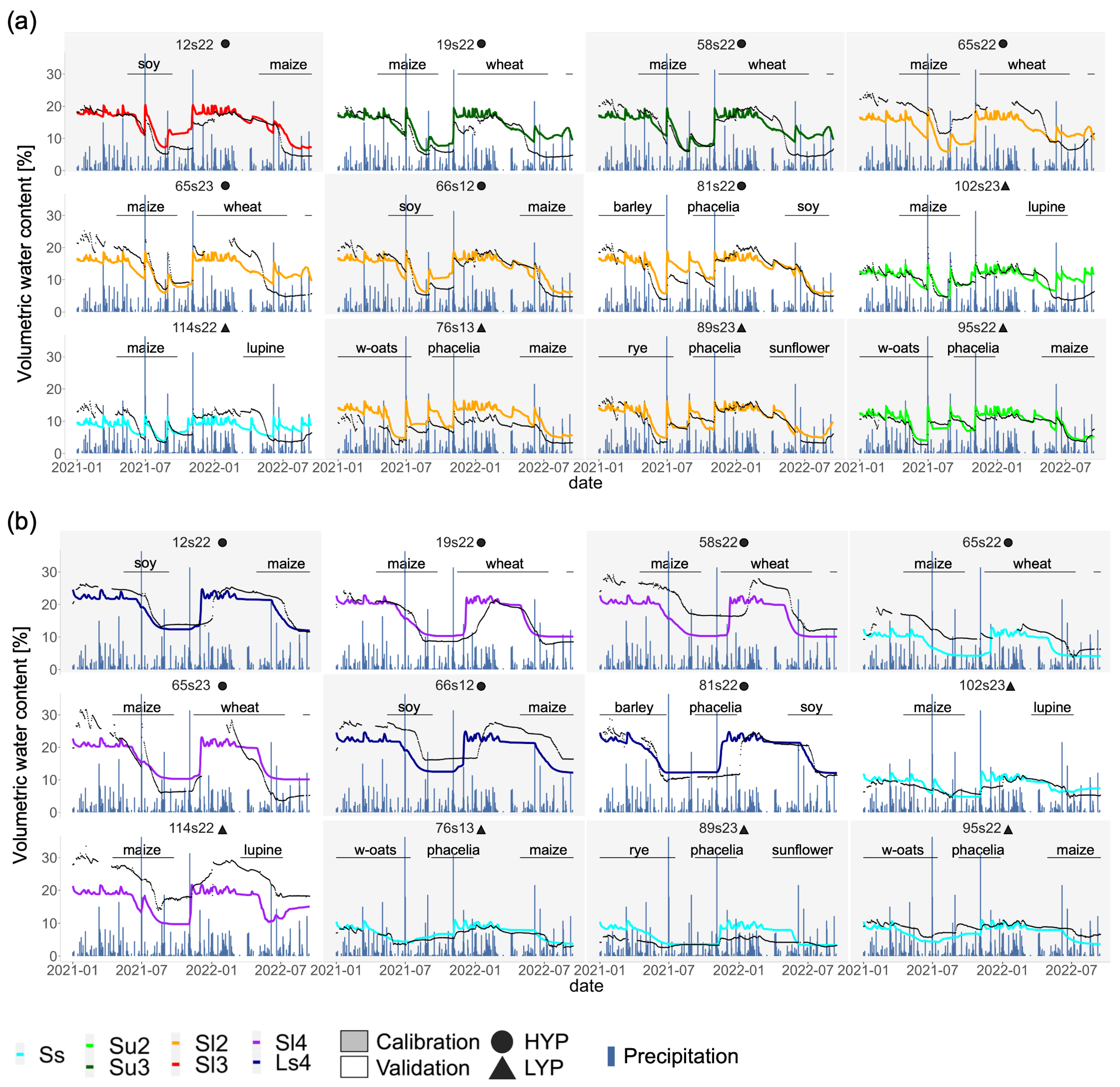
3.1. Observed Soil Moisture Dynamics

The observed SWC was highly variable among locations, depth and during the season (Figure S2). Generally, the SWC was highest during the winter months and started to be depleted during the crop growth period in spring and summer in both top- and subsoil. During the phacelia growing period, the SWC decreased at 30 cm depth, but remained stable or slightly increased at 90 cm depth. The daily SWC ranged from 2.6% in patch 89 in June 2021 to 33.5% in patch 114 in May 2021, both recorded at 90 cm depth. Particularly, the data recorded at 30 cm depth showed peaks in SWC coinciding with major precipitation events, but this was not the case at 60 and 90 cm depth, except for very sandy locations. Sensors located in loamy subsoil recorded larger absolute ranges in the SWC, while in the very sandy locations (Ss) the observed SWC was more stable. During crop growth, fast decreases in SWC occurred at all depths, likely due to crop water extraction. The right sensor in patch 65 was an exception, since during maize crop growth no decrease in SWC at 60 cm was observed, even though the left sensor of the same patch showed strong water extraction. Also, the two sensors at 90 cm depth recorded distinct differences regarding the maximum and minimum SWC, even though they were only a few meters apart, likely caused by heterogeneous soil conditions. While they were located next to very different soil profiles (Ss vs. strongly loamy sand (Sl4) at 90 cm depth), the sensor in the sandy subsoil showed a higher observed SWC than other locations with sandy subsoil and the sensor located close to a Sl4 texture in the subsoil, which showed a lower minimum SWC (min. 3.5%) than the other Sl4 locations.

3.2. Pedotransfer Functions and Soil Hydraulic Properties

The field capacity and available water capacity (AWC) varied among soil textural classes and PTF setup, ranging from 8% to 24% and 5% to 13%, respectively (Figure 2). For Hypres1315 and 1517, an increasing sand content always led to a lower field capacity and AWC; however, for BK, this relationship was less pronounced.

For the Hypres PTF, the Hypres1517 setting generally produced slightly lower field capacity values (~2%) than the Hypres1315 in the topsoil, while differences due to bulk density in the subsoil were smaller, especially for texture classes with a high sand content (Figure 2). The differentiation in soil particle size distribution by yield potential zone within a soil textural class had the largest impact on slightly loamy sand (Sl2), which resulted in up to 2.5% higher field capacity and AWC when based on samples within the high yield potential zone. For the class-based BK PTF, no differentiation in hydraulic properties within a soil textural class was possible. With increasing sand content, the field capacity assigned to the texture classes either remained stable or decreased, but the range of field capacity values was smaller compared to both Hypres setups. Also, contrarily to the Hypres setups, the AWC did not always decrease with increasing sand content. While the BK assigned the same field capacity to the classes Sl4 and strongly sandy loam (Ls4), the AWC differed strongly with Ls4 showing the lowest AWC of all soil textural classes, which was the opposite in both Hypres setups, where the Ls4 was among the soil textural classes with the highest AWC (Figure 2d).

3.3. Effect of Pedotransfer Function and Bulk Density on SWC Simulation

The different pedotransfer setups used in terms of PTF and bulk density input to derive soil hydraulic properties led to differences in the simulated soil water content. The model performed best when using the setup Hypres1517 as evident from all statistical indicators of model performance in the calibration, except for the mean error (

Table 6. Model performance indicators for model calibration and validation of daily soil water content for selected locations at the patchCROP experiment, Tempelberg, Brandenburg.

Pedotransfer Setup 1	Calibration/ Validation	rRMSE 2	R2	Error 3	EF 4	MAE 5	N
BK	Calibration	35.6	0.64	1.68	0.58	3.40	10,136
	Validation	36.2	0.66	2.21	0.54	3.58	7240
Hypres1315	Calibration	31.4	0.67	−0.01	0.67	2.99	10,136
	Validation	31.6	0.66	0.57	0.65	2.84	7240
Hypres1517	Calibration	29.5	0.72	−0.41	0.71	2.76	10,136
	Validation	32.5	0.64	0.19	0.63	2.96	7240

¹ BK = based on the German manual of soil mapping KA5; Hypres1315 = Hypres pedotransfer function with bulk density of 1.3 g/cm³ in the topsoil layer and 1.5 g/cm³ in the subsoil layers; Hypres1517 = Hypres pedotransfer function with bulk density of 1.5 g/cm³ in the topsoil layer and 1.7 g/cm³ in the subsoil layers; ² relative root mean squared error (rRMSE in %); ³ mean error (error in t ha⁻¹); ⁴ model efficiency (EF); ⁵ mean absolute error (MAE in t ha⁻¹).

). Using Hypres1517 led to an average underestimation of soil moisture by 0.41 Vol%, showed lowest rRMSE of 29.6%, the highest R² (0.72) and the lowest MAE of 2.76 Vol% during calibration. Furthermore, this setup obtained the highest model efficiency of 0.71. The Hypres setup with lower bulk density performed slightly worse in all statistical aspects for calibration, except for the mean error.

The major difference in model performance of Hypres1517 and Hypres1315 during calibration appears to be the simulation of SWC for the soil textural classes slightly silty sand (Su2) and medium loamy sand (Sl3), which are present at 30 cm depth (Figure S3). For simulating SWC in Su2, Hypres1315 showed an rRMSE of 33.7% in calibration, while the setup with higher bulk density performed better, with an rRMSE of 17.13%. The setup with lower bulk density tended to overestimate the SWC (mean error = 2.6 Vol%). The same was true when simulating the SWC for Sl3. Here, the mean error during calibration for setup Hypres1315 was 3.5 Vol%, while Hypres1517 had a lower mean error of 2.2, resulting in a lower rRMSE (22.5% vs. 31.2%). The BK input led to the poorest model performance during calibration, with the highest rRMSE of 35.6%, the highest average overestimation of soil moisture (mean error = 1.68 Vol%), the highest MAE of 3.4 Vol% and the lowest R² and EF with 0.64 and 0.58, respectively. The same trends were apparent in the validation dataset, where errors with BK simulation were even slightly larger. One major source for this was the BK model’s performance under very sandy (Ss) conditions (Figure S3), as the SWC was frequently overestimated, leading to high errors (rRMSE of 39.5% in validation) and negative model efficiency (EF) during both calibration and validation (−0.31 and −0.03), which indicates that using the mean of observed data for Ss would have been a better predictor than the model. As shown in Figure 3 for the SWC at two contrasting (Ss vs. Ls4 subsoil texture) soil profiles within the calibration set during maize growth, the BK model performed worse at predicting SWC for Ss and Ls4. For location 12s22 with Ls4 at 90 cm depth, all predictions matched the observed SWC when maize was sown, but, using the BK setup, the predicted SWC did not decrease as much as observed in the following months. The opposite was the case for predicting the SWC in profile 76s13 with Ss at 90 cm depth. Here, the BK setup overestimated the SWC at sowing time but reached the same level during the crops’ water extraction, overestimating the available water during maize growth. Although in the calibration set the Hypres1517 performed better than the setup with lower bulk density, this trend was not so clear for the validation set, where the rRMSE, R² and EF were slightly better for the Hypres1315 setup, although the mean error was still lower for the Hypres1517 setup.

The observed and simulated SWC for each location using the Hypres1517 setup, which performed best during calibration, are shown in Figure 4. Generally, the maximum and minimum simulated SWC mostly matched with the observed range for the respective location, indicating that the hydraulic properties estimated with the Hypres1517 setup were similar to the actual conditions. Major differences were apparent for location 65s22 (Sl2) at 30 cm depth and for 58s22 (Sl4), 65s22 (Ss), 65s23 (Sl4) and 114s22 (Sl4) at 90 cm depth (Figure 4). At 30 cm depth, the peaks in SWC after precipitation events were captured by the model, as well as decreases in the SWC during crop presence. The SWC patterns at 30 cm depth during crop presence matched particularly well during growth of maize, winter barley, winter rye, soybean (2022), phacelia and winter oats (Figure 4). At 30 cm depth, the model showed worse performance during the growth of winter wheat, lupine (2022) and soybean (2021), which was mainly due to the overestimation of SWC during summer. Considerable prediction errors during the growth of soybean occurred towards the end of the growing season, but only in 2021. These trends did not occur at 90 cm depth. When only considering the locations where the simulation and observation of minimum and maximum SWC were similar at 90 cm depth (12s22, 19s22, 81s22, 102s23, 76s13, 95s22), the patterns and timing of the SWC decrease and increase during crop presence were mostly well reproduced by the model. Nevertheless, substantial overestimation of SWC by the model occurred in winter 2021 after a heavy rain event (31.4 mm on 4 November 2021) at all locations where Sl4 or Ls4 was present in the subsoil (Figure 4). Furthermore, the two locations in patch 65 (65s22 and 65s23), which showed contrasting soil textures in subsoils Ss and Sl4, respectively, also showed some noticeable patterns in the observed SWC. At the location with Ss as the subsoil texture, the model tended to underestimate the SWC (MAE = 4.07 Vol%), while at the location with Sl4 in the subsoil, the SWC was both substantially over- and underestimated. At the remaining locations with Ss at 90 cm depth, the SWC was simulated fairly accurately, with an MAE ranging from 0.88 (76s13) to 2.05 Vol% (89s23). When comparing the model performance among soil textural classes, the rRMSE did not provide a reliable indication of performance as small absolute errors led to considerably higher rRMSE values for locations where a low SWC was observed. This becomes apparent when comparing the model performance at 90 cm depth at locations 114s22 and 89s23. While the sandy 89s23 showed an MAE of 2 Vol%, the rRMSE was 61.8%. The loamier location 114s22 shows larger discrepancies in simulated SWC, with an MAE of 7.2 Vol% but a lower rRMSE of 33% (Figure 4b).

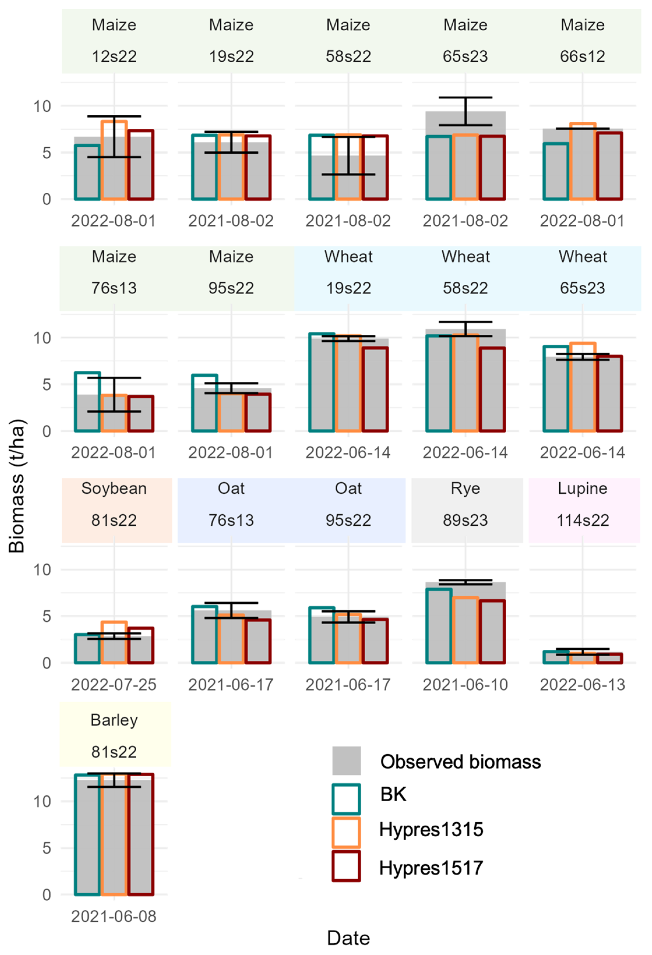
3.4. Observed Above Ground Biomass

The observed above ground biomass around flowering ranged from 1.2 t/ha (n = 4) of lupine in patch 114 in June 2022 to 12.3 t/ha (n = 4) of barley in patch 81 in June 2021 (Figure 5). Out of the 16 biomass samplings conducted in this study, maize was the most frequent crop, with seven sampling events in 2021 and 2022, as it is part of both the low and high yield potential rotation and was grown across a wide range of soil conditions. The maize biomass in both 2021 and 2022 was collected in the beginning of August at the end of flowering/beginning of fruit development and ranged from 3.9 t/ha (n = 4) in sandy patch 76 to 9.4 t/ha (n = 2) in the loamier patch 65 in 2022 (Figure 5, Table S2). While most crops showed rather low standard deviations due to variation among the repetitions, the standard deviation of observed biomass was especially high for maize in the patches 12, 58, 65 and 76. Except for winter oat, which showed a biomass of around 5 t/ha at both locations in 2021, the winter crops winter wheat and winter rye exhibited higher above ground biomass after flowering, with circa 10 t/ha and circa 8 t/ha, respectively (Figure 5).

3.5. Effect of Pedotransfer Function and Bulk Density on Biomass Simulations

The different PTF setups led to differences in simulated biomass, with the global rRMSE ranging from 19.6% for the BK setup to 18.2% for the Hypres1315 setup (

Table 7. Model performance indicators for above ground biomass after flowering at the patchCROP experiment, Tempelberg, Brandenburg.

Pedotransfer Setup 1	rRMSE 2	R2	Error 3	MAE 4	N
BK	19.6	0.80	0.23	1.07	16
Hypres1315	18.2	0.84	0.20	0.97	16
Hypres1517	18.5	0.84	−0.35	0.97	16

¹ BK = based on the German manual of soil mapping KA5; Hypres1315 = Hypres pedotransfer function with bulk density of 1.3 g/cm³ in the topsoil layer and 1.5 g/cm³ in the subsoil layers; Hypres1517 = Hypres pedotransfer function with bulk density of 1.5 g/cm³ in the topsoil layer and 1.7 g/cm³ in the subsoil layers; ² relative root mean squared error (rRMSE in %); ³ mean error (error in t ha⁻¹), ⁴ mean absolute error (MAE in t ha⁻¹).

). While the Hypres1517 did show a tendency to underestimate the biomass (Error = −0.35 t/ha) and had a slightly higher rRMSE with 18.5% compared to Hypres1315, R² was marginally higher and the MAE was the same for both Hypres setups (0.97 t/ha). The BK setup performed slightly worse than the two Hypres setups in all performance indicators assessed, with an rRMSE of 19.6%, an MAE of 1.07 t/ha and a lower R² (0.80).

For the prediction of barley biomass in 2021, the PTF setup did not have a relevant impact, while for maize, winter wheat, soybean, winter oat and winter rye differences were apparent, although in some locations the difference in biomass simulation due to model setup were all within the standard deviation of the observed biomass (Figure 5). Comparing the two Hypres setups, the higher bulk density led to either no difference in biomass predictions or a reduction in biomass. This effect was more pronounced at locations featuring rather loamy soil textural classes, which is in line with the higher impact of bulk density on available water capacity for soil textural classes with lower sand content (Figure 2). The biggest difference regarding accuracy of biomass predictions due to bulk density was found within the texture class Ls4, where the Hypres1517 setup performed better compared to Hypres1315 (rRMSE 9.1 and 16.3%, Table S3). Regarding the simulation of maize biomass, both Hypres setups better captured the impact of soil heterogeneity on crop growth than the BK. Using the Hypres1517 setup, the model predicted a maize biomass of 3.7 t/ha for the sandy location (76s13) and 7.1 t/ha for the location with loamy subsoil (66s12) in 2022, which was similar to the observed biomass, while using the BK setup the soil conditions did not lead to differentiation, with a predicted biomass of 6.2 and 6 t/ha, respectively. The predicted biomass was even higher in the sandy than the loamy location, which was not reflected by the observations. The available water capacity when applying the BK PTF was surprisingly low for textural class Ls4 (7%) (Figure 2), even though the field capacity was similar to other setups, as previously highlighted regarding the SWC simulation (Figure 3). While the biomass predictions were lower using the BK compared to the Hypres PTF in profiles with Ls4 in the last layer, it did not lead to a major increase in prediction error for biomass (Table S3). Instead, the relatively high available water capacity for the texture class Ss led to biomass over predictions, which also led to a relatively high rRMSE of 24.6% when using the BK at locations with Ss as the subsoil texture (Table S3), consequently limiting the sensitivity to capture differences in biomass due to soil conditions. While the Hypres setups were able to capture differences between very contrasting soil conditions, in locations with loamy subsoil the predicted biomass was often similar.

Overall, the continuous Hypres PTF with bulk densities of 1.5 g/cm³ in the topsoil and 1.7 g/cm³ in the subsoil proved to be advantageous over the Hypres setup with lower bulk densities and the class-based PTF BK for simulating soil water dynamics. While small differences were observed in the prediction of biomass, both Hypres setups still proved to be advantageous over the BK setup, as they were better able to capture biomass variation among different locations.

4. Discussion

Previous research has shown that agro-ecosystem models differ in their ability to capture the impact of soil heterogeneities on soil moisture and crop growth [61]. Additionally, while previous studies have performed sensitivity analyses regarding PTF choice and its influence on simulating the SWC and/or biomass of agro-ecosystem models, in this study, we additionally assessed the performance of PTF functions under heterogeneous conditions by using an extensive soil moisture time series in top- and subsoil and accuracy of biomass predictions in the context of within-field heterogeneity by accounting for a wide range of crops, showing that the PTF performance also varies depending on the soil characteristics. We found that both soil moisture and biomass simulations were dependent on the PTF selection to derive soil hydraulic properties. Additionally, the use of a tipping-bucket model with the Hypres PTF enabled the model to capture the impacts of soil-related within-field heterogeneities on soil water dynamics in the top- and subsoil and on above ground biomass.

Regarding the simulation of soil water content, the model performance was dependent on the used PTF, with an EF ranging from 0.54 to 0.66 after calibration. While the simulated soil moisture dynamics were similar, the range of simulated SWC was influenced by the model setup. Even though Hypres is based on a European soil database and BK was developed for German soil texture classes, using the continuous Hypres PTF [34] proved to be advantageous over the class-based BK. This is in line with Weihermüller et al. [31], who tested the influence of PTF on the simulation of water balance fluxes using a Richards’ equation-based model (HYDRUS-1D [62]) and found that the PTF substantially affected the simulation of water fluxes. Furthermore, they classified the Hypres PTF as overall robust, while two class-based PTFs were classified as non-robust. In our study, the available water capacity when applying the BK PTF was surprisingly low for the textural class Ls4 (7%), even though the field capacity was similar to other setups. While the BK provides another table where a differentiation of bulk density within a texture class is possible, this table refers to a field capacity at pF 1.8, while the SimComponent SlimWater requires a field capacity at pF 2.5. Therefore, this approach did not allow us to differentiate for bulk density, but was rather based on an average of 1.5 g/cm³, potentially limiting its performance. A new edition of the BK has been released in August 2024, with updated look-up tables to derive soil hydraulic properties based on soil textural class, and it provides a table based on pF 2.5 with the ability to differentiate bulk density classes [63]. Future research should assess whether the revised soil hydraulic properties provide reasonable soil input for crop models, as this approach could reduce cost and labor intensive laboratory analysis of particle size distribution. Most continuous PTFs require input for the bulk density [30], and while the impact of bulk density was not as large as the PTF selection, model performance was impacted. The PTF with a higher bulk density of 1.5 g/cm³ in the topsoil and 1.7 g/cm³ in the subsoil outperformed the lower bulk density, with relevant differences in model performance occurring for the simulation of SWC in the textural classes Sl3 and Su2, leading to an increased EF. Koszinski et al. investigated field-scale bulk density heterogeneity under similar soil conditions [64]. The bulk density results agreed with choosing the higher bulk density setup in this study. Additionally, while they did find bulk density to be structurally variable dependent on soil depth and number of roots, variance within the field (headlands excluded) was low, indicating that using a depth-dependent bulk density as model input was reasonable, as long as it was for simulating the main field rather than headlands. Independently of the PTF setup, the simulations showed a too early onset of SWC increase after heavy rain in the loamier subsoils, which can be assumed to be due to the model structure, namely, the cascading process of the tipping-bucket approach implemented in SlimWater. Romano et al. compared the model performance of a tipping-bucket and Richards’ equation-based model and found that the tipping-bucket model had smaller memory capability, therefore reacting more rapidly to climatic forcing in both increases and decreases in SWC [65]. Vianna et al. tested how the soil moisture prediction was affected by model structure and data detail [27]. They found that the prediction of soil moisture was only slightly improved by applying the SWAP platform (Richard’s equation based, rRMSE = 6%) rather than a tipping-bucket approach (rRMSE = 8%). While the rRMSE was lower compared to our study, it has to be noted that the soil moisture range was much higher (from 0.2 to 0.4 cm³/cm³), limiting the comparability of the rRMSE. With an ME of 0.7, the tipping-bucket approach performed similarly. Furthermore, they concluded that a tipping-bucket approach may be preferred when soil parameters are limited, as has been the case in this study. While location 12s22 was analyzed for sand, silt and clay fractions of each layer, the remaining locations relied on an extrapolation of the particle size distribution, introducing additional uncertainty. In particular, Sl4 at 90 cm depth shows high heterogeneity in the range of observed SWC among the locations. While one possible explanation could be errors in the measured volumetric soil water content, due to limitations such as standard error of 1–3 Vol.% when employing TDR sensors [66], the texture class Sl4 did exhibit relatively high variance for particle size fractions (Figure S1), indicating that using a uniform particle size distribution limited the prediction accuracy. The importance of soil input was also highlighted by Stahn et al., who, based on a sensitivity analysis, found soil properties to be most relevant for predicting soil water content in the agro-hydrological model SWAP [67]. Nevertheless, when aiming to simulate within-field heterogeneity for a considerable field size, it can be expected that model soil input will come with greater uncertainty, as it is not feasible to use traditional methods for each point of simulation [15], but rather proximal sensing technologies [68,69]. Despite the small distance of 5 m between the locations 65s22 and 65s23, they exhibited great differences in subsoil texture and SWC. The SWC was underestimated by the model in the location with sandy subsoil but overestimated during relatively dry periods in the location with loamy subsoil. While there could be many factors at play, one explanation might be lateral subsurface flow, which is known to occur in hummocky ground moraine landscapes [70] and is not captured by the model.

The simulated and observed SWC during crop growth differed strongly, particularly during the growth of winter wheat, lupine and soybean in 2021. The simulation of lupine showed very limited above ground biomass at flowering for location 102s23 (0.35 t/ha at maturity), which led to low transpiration and low water extraction, therefore increasing SWC due to precipitation. While location 114s22 showed the same pattern at 30 cm depth, strong decreases in SWC were observed at 90 cm depth in simulated and observed data. Nevertheless, the timing of decrease differed, as well as the absolute values. While the timing might point to issues in the simulation of crop development, differences in absolute values at this location were apparent during the whole time period, indicating these were most likely due to soil input as discussed above, rather than crop extraction. Prediction errors during the late growing period of soybean could be due to inaccuracies in phenology simulation, as soybean reached maturity 10 days prematurely in the simulation. These crop-specific errors occurring at different soil conditions underline the complexity, as not only soil, but also crop parameters, introduce uncertainty and errors. This is in line with Groh et al., who performed a model intercomparison and found that a crop parametrization solely on crop phenology data led to inadequate simulation of SWC [71]. Although soil data were detailed and complex models were tested, the multi-model mean of rRMSE was circa 50% for the simulation of SWC. Similarly, Wegehenkel et al. found SWC simulation errors in summer due to root water extraction [72].

The use of different PTF approaches also influenced the simulation of the above ground biomass. While for simulating the SWC Hypres1517 performed best in the calibration stage, for the simulation of biomass, the Hypres1315 setup performed slightly better, even though the differences between the two were minimal. The BK setup, on the other hand, showed the lowest performance for SWC and also for the simulation of biomass, specifically when considering the ability to reproduce the effect of different soil properties (sandy vs. loamy) on biomass. Even though all the PTF setups showed a trend of decreasing field capacity with increasing sand content, this was not the case for the available water capacity within the PTF BK (Figure 2), for which the differentiation of available water capacity among soil texture classes was rather small. This is in line with other studies that have found the available water capacity to be one of the most important factors influencing crop model output [61,73]. The major difference in biomass prediction due to the PTF approach was found for locations with sandy subsoil, which is consistent with Rosso et al., who found yield predictions to be most affected by the applied PTF approach under sandy conditions [38]. While it could have been suspected that the too early onset of SWC increase when predicting SWC in loamy subsoils (which occurred independently of the applied PTF approach) would lead to an overestimation of the simulated above ground biomass due to higher amounts of plant available water, this was not supported by the simulated crop growth. A likely explanation is the timing of overestimation, which occurred either during a fallow period or right before the sowing of winter wheat in November (patches 19, 58 and 65). In the following months, the simulated winter wheat roots did not reach the depth where the loamier texture appeared, so it did not impact crop growth. This is in line with Wallor et al., who found that the level of prediction accuracy regarding soil-related process did not always correspond with the prediction accuracy of the yield [61].

While we did observe some limitations in the simulation of soil water dynamics (lateral flow, loamy conditions) due to employing a tipping-bucket approach, the model was able to reasonably reproduce the spatial-temporal dynamics of soil moisture, as well as the above ground biomass. In future steps, we plan to combine the model with a high-resolution soil map to assess spatial and temporal management adaptations (e.g., nitrogen fertilizer, crop allocation) at a larger scale. When simulating crop performance as influenced by potential nitrogen limitations (which is the case in this model setup), the model needs to be able to simulate soil nitrogen dynamics, which are more commonly tested and applied in tipping-bucket approach models [74]. More advanced soil hydrological models often lack the simulation of soil nitrogen dynamics, and require more detailed soil information and substantially higher computational power due to sub-daily time steps [26,27]. While no hardware or computational constraints were encountered in the current study, for future model applications the scale and complexity of simulations will increase and computational requirements are expected to grow significantly, potentially requiring the use of high-performance computing. As (1) the groundwater table in this location is well below the root zone, (2) the detail of soil data is limited, (3) the model needs to account for soil nitrogen dynamics and (4) the simulation complexity will increase for future applications, we chose a tipping-bucket approach, which is commonly utilized in crop modelling applications [23,50] and assessed it to be an adequate option for the simulation of soil water dynamics and crop growth within the context of a ground moraine characterized by a high degree of soil heterogeneity.

The findings highlight the importance of within-field soil, especially subsoil, heterogeneity and the consequent variability of soil moisture and crop available water, which needs to be accounted for as it potentially limits crop growth depending on the seasonal rainfall and weather conditions. The calibrated and validated agroecosystem models can be used to design diversified cropping systems by considering the interaction between soil heterogeneities and interannual variability affecting soil water dynamics in the top- and subsoil and, therefore, crop growth and productivity. Also, the agro-ecosystem model can be utilized for assessing management adaptations, such as improved site-specific fertilizer practices, in both the spatial and temporal context.

5. Conclusions

When spatializing agro-ecosystem models, the simulation of soil moisture often receives too little attention in model performance assessment. Coming from different research questions, studies have come to different conclusions on the needed complexity of model structure and input data. In this study, we found that the model was able to capture the within-field variability in SWC reasonably well over two growing seasons under different crops and heterogeneous soil conditions when using a model that applies a tipping-bucket approach for SWC simulation, which was also previously calibrated for crop growth. The choice of pedotransfer function proved to be important for the simulation of soil water content and, in some cases, translated to differences in prediction accuracy for above ground biomass as well. For the simulation of daily soil water dynamics, the model error was largest after intense rain events for soils with a loamy texture in the subsoil, as the increase in simulated SWC levels occurred too early, probably due to the capacity-based cascading process that simulates percolation. While the model’s biomass predictions did not appear to be negatively influenced by this error, further model testing and improvement might be useful, as extreme precipitation events may occur more often under future climatic conditions or when simulation is focused on other model outputs, such as N leaching. Some uncertainties were introduced due to soil input and crop growth; nevertheless, the calibrated model using the Hypres PTF was able to reproduce reasonably well the interactive effect of climate, management (crop rotation) and contrasting soil conditions on site-specific daily soil moisture dynamics across the studied growing seasons, as well as on intermediate biomass productivity. The tested model has the potential to be used for further studies on how SWC dynamics can be affected by management practices under heterogeneous soil conditions.

References

1. FAO. The Future of Food and Agriculture: Trends and Challenges; FAO: Rome, Italy, 2017. [Google Scholar]
2. Schiller, J.; Jänicke, C.; Reckling, M.; Ryo, M. Higher Crop Rotational Diversity in More Simplified Agricultural Landscapes in Northeastern Germany. Landsc. Ecol. 2024, 39, 1–18. [Google Scholar] [CrossRef]
3. Tamburini, G.; Bommarco, R.; Wanger, T.C.; Kremen, C.; van der Heijden, M.G.A.; Liebman, M.; Hallin, S. Agricultural Diversification Promotes Multiple Ecosystem Services without Compromising Yield. Sci. Adv. 2020, 6, eaba1715. [Google Scholar] [CrossRef] [PubMed]
4. Basso, B.; Antle, J. Digital Agriculture to Design Sustainable Agricultural Systems. Nat. Sustain. 2020, 3, 254–256. [Google Scholar] [CrossRef]
5. Clough, Y.; Kirchweger, S.; Kantelhardt, J. Field Sizes and the Future of Farmland Biodiversity in European Landscapes. Conserv. Lett. 2020, 13, e12752. [Google Scholar] [CrossRef]
6. Tscharntke, T.; Grass, I.; Wanger, T.C.; Westphal, C.; Batáry, P. Beyond Organic Farming–Harnessing Biodiversity-Friendly Landscapes. Trends Ecol. Evol. 2021, 36, 919–930. [Google Scholar] [CrossRef]
7. Sirami, C.; Gross, N.; Baillod, A.B.; Bertrand, C.; Carrié, R.; Hass, A.; Henckel, L.; Miguet, P.; Vuillot, C.; Alignier, A.; et al. Increasing Crop Heterogeneity Enhances Multitrophic Diversity across Agricultural Regions. Proc. Natl. Acad. Sci. USA 2019, 116, 16442–16447. [Google Scholar] [CrossRef] [PubMed]
8. Groß, J.; Gentsch, N.; Boy, J.; Heuermann, D.; Schweneker, D.; Feuerstein, U.; Brunner, J.; Von Wirén, N.; Guggenberger, G.; Bauer, B. Influence of Small–Scale Spatial Variability of Soil Properties on Yield Formation of Winter Wheat. Plant Soil 2023, 493, 79–97. [Google Scholar] [CrossRef]
9. Milics, G.; Kovacs, A.J.; Pörneczi, A.; Nyeki, A.; Varga, Z.; Nagy, V.; Lichner, L.; Nemeth, T.; Baranyai, G.; Nemenyi, M. Soil Moisture Distribution Mapping in Topsoil and Its Effect on Maize Yield. Biologia 2017, 72, 847–853. [Google Scholar] [CrossRef]
10. Adamchuk, V.I.; Ferguson, R.B.; Hergert, G.W. Soil Heterogeneity and Crop Growth. In Precision Crop Protection–The Challenge and Use of Heterogeneity; Oerke, E., Gerhards, R., Menz, G., Sikora, R., Eds.; Springer: Dordrecht, The Netherlands, 2010; pp. 3–16. [Google Scholar] [CrossRef]
11. Nordmeyer, H.; Richter, J. Incubation Experiments on Nitrogen Mineralization in Loess and Sandy Soils. Plant Soil 1985, 83, 433–445. [Google Scholar] [CrossRef]
12. Paul, K.I.; Polglase, P.J.; O’Connell, A.M.; Carlyle, J.C.; Smethurst, P.J.; Khanna, P.K. Defining the Relation between Soil Water Content and Net Nitrogen Mineralization. Eur. J. Soil Sci. 2003, 54, 39–48. [Google Scholar] [CrossRef]
13. Kersebaum, K.C.; Lorenz, K.; Reuter, H.I.; Schwarz, J.; Wegehenkel, M.; Wendroth, O. Operational Use of Agro-Meteorological Data and GIS to Derive Site Specific Nitrogen Fertilizer Recommendations Based on the Simulation of Soil and Crop Growth Processes. Phys. Chem. Earth 2005, 30, 59–67. [Google Scholar] [CrossRef]
14. Basso, B.; Ritchie, J.T.; Pierce, F.J.; Braga, R.P.; Jones, J.W. Spatial Validation of Crop Models for Precision Agriculture. Agric. Syst. 2001, 68, 97–112. [Google Scholar] [CrossRef]
15. Kersebaum, K.C.; Wallor, E. Process-Based Modelling of Soil–Crop Interactions for Site-Specific Decision Support in Crop Management. In Precision Agriculture: Modelling; Cammarano, D., van Evert, F.K., Kempenaar, C., Eds.; Springer: Berlin/Heidelberg, Germany, 2023; pp. 25–47. [Google Scholar] [CrossRef]
16. Jarvis, N.; Coucheney, E.; Lewan, E.; Klöffel, T.; Meurer, K.H.E.; Keller, T.; Larsbo, M. Interactions between Soil Structure Dynamics, Hydrological Processes, and Organic Matter Cycling: A New Soil-Crop Model. Eur. J. Soil Sci. 2024, 75, e13455. [Google Scholar] [CrossRef]
17. Bethwell, C.; Burkhard, B.; Daedlow, K.; Sattler, C.; Reckling, M.; Zander, P. Towards an Enhanced Indication of Provisioning Ecosystem Services in Agro-Ecosystems. Environ. Monit. Assess. 2021, 193, 269. [Google Scholar] [CrossRef] [PubMed]
18. Gao, F.; Luan, X.; Yin, Y.; Sun, S.; Li, Y.; Mo, F.; Wang, J. Exploring Long-Term Impacts of Different Crop Rotation Systems on Sustainable Use of Groundwater Resources Using DSSAT Model. J. Clean. Prod. 2022, 336, 130377. [Google Scholar] [CrossRef]
19. Olesen, J.E.; Trnka, M.; Kersebaum, K.C.; Skjelvåg, A.O.; Seguin, B.; Peltonen-Sainio, P.; Rossi, F.; Kozyra, J.; Micale, F. Impacts and Adaptation of European Crop Production Systems to Climate Change. Eur. J. Agron. 2011, 34, 96–112. [Google Scholar] [CrossRef]
20. Vereecken, H.; Schnepf, A.; Hopmans, J.W.; Javaux, M.; Or, D.; Roose, T.; Vanderborght, J.; Young, M.H.; Amelung, W.; Aitkenhead, M.; et al. Modeling Soil Processes: Review, Key Challenges, and New Perspectives. Vadose Zone J. 2016, 15, vzj2015-09. [Google Scholar] [CrossRef]
21. Ginaldi, F.; Bajocco, S.; Bregaglio, S.; Cappelli, G. Spatializing Crop Models for Sustainable Agriculture. In Innovations in Sustainable Agriculture; Farooq, M., Pisante, N., Eds.; Springer Nature: Berlin, Germany, 2019; pp. 599–619. [Google Scholar] [CrossRef]
22. Falco, N.; Wainwright, H.M.; Dafflon, B.; Ulrich, C.; Soom, F.; Peterson, J.E.; Brown, J.B.; Schaettle, K.B.; Williamson, M.; Cothren, J.D.; et al. Influence of Soil Heterogeneity on Soybean Plant Development and Crop Yield Evaluated Using Time—Series of UAV and Ground—Based Geophysical Imagery. Sci. Rep. 2021, 11, 7046. [Google Scholar] [CrossRef]
23. Tenreiro, T.R.; García-Vila, M.; Gómez, J.A.; Jimenez-Berni, J.A.; Fereres, E. Water Modelling Approaches and Opportunities to Simulate Spatial Water Variations at Crop Field Level. Agric. Water Manag. 2020, 240, 106254. [Google Scholar] [CrossRef]
24. Jarvis, N.; Larsbo, M.; Lewan, E.; Garre, S. Improved Descriptions of Soil Hydrology in Crop Models: The Elephant in the Room? Agric. Syst. 2022, 202, 103477. [Google Scholar] [CrossRef]
25. Siad, S.M.; Iacobellis, V.; Zdruli, P.; Gioia, A.; Stavi, I.; Hoogenboom, G. A Review of Coupled Hydrologic and Crop Growth Models. Agric. Water Manag. 2019, 224, 105746. [Google Scholar] [CrossRef]
26. Wallach, D.; Makowski, D.; Jones, J.W.; Brun, F. Working with Dynamic Crop Models: Methods, Tools and Examples for Agriculture and Environment, 3rd ed.; Academic Press–Elsevier: London, UK, 2019. [Google Scholar] [CrossRef]
27. Vianna, M.d.S.; Metselaar, K.; de Jong van Lier, Q.; Gaiser, T. The Importance of Model Structure and Soil Data Detail on the Simulations of Crop Growth and Water Use: A Case Study for Sugarcane. Agric. Water Manag. 2024, 301, 108938. [Google Scholar] [CrossRef]
28. Longo, M.; Jones, C.D.; Izaurralde, R.C.; Cabrera, M.L.; Dal Ferro, N.; Morari, F. Testing the EPIC Richards Submodel for Simulating Soil Water Dynamics under Different Bottom Boundary Conditions. Vadose Zone J. 2021, 20, e20142. [Google Scholar] [CrossRef]
29. Soldevilla-Martinez, M.; Quemada, M.; Lopez-Urrea, R.; Munoz-Carpena, R.; Lizaso, J.I. Soil water balance: Comparing two simulation models of different complexity with lysimeter observations. Agric. Water Manag. 2014, 139, 53–63. [Google Scholar] [CrossRef]
30. Van Looy, K.; Bouma, J.; Herbst, M.; Koestel, J.; Minasny, B.; Mishra, U.; Montzka, C.; Nemes, A.; Pachepsky, Y.A.; Padarian, J.; et al. Pedotransfer Functions in Earth System Science: Challenges and Perspectives. Rev. Geophys. 2017, 55, 1199–1256. [Google Scholar] [CrossRef]
31. Weihermüller, L.; Lehmann, P.; Herbst, M.; Rahmati, M.; Verhoef, A.; Or, D.; Jacques, D.; Vereecken, H. Choice of Pedotransfer Functions Matters When Simulating Soil Water Balance Fluxes. J. Adv. Model. Earth Syst. 2021, 13, e2020MS002404. [Google Scholar] [CrossRef]
32. Schaap, M.G.; Leij, F.J.; van Genuchten, M.T. Rosetta: A Computer Program for Estimating Soil Hydraulic Parameters with Hierarchical Pedotransfer Functions. J. Hydrol. 2001, 251, 163–176. [Google Scholar]
33. Tóth, B.; Weynants, M.; Nemes, A.; Makó, A.; Bilas, G.; Tóth, G. New Generation of Hydraulic Pedotransfer Functions for Europe. Eur. J. Soil Sci. 2015, 66, 226–238. [Google Scholar] [CrossRef]
34. Wösten, J.H.M.; Lilly, A.; Nemes, A.; Le Bas, C. Development and Use of a Database of Hydraulic Properties of European Soils. Geoderma 1999, 90, 169–185. [Google Scholar] [CrossRef]
35. Contreras, C.P.; Bonilla, C.A. A Comprehensive Evaluation of Pedotransfer Functions for Predicting Soil Water Content in Environmental Modeling and Ecosystem Management. Sci. Total Environ. 2018, 644, 1580–1590. [Google Scholar] [CrossRef]
36. Román Dobarco, M.; Cousin, I.; Le Bas, C.; Martin, M.P. Pedotransfer Functions for Predicting Available Water Capacity in French Soils, Their Applicability Domain and Associated Uncertainty. Geoderma 2019, 336, 81–95. [Google Scholar] [CrossRef]
37. Ramos, T.B.; Darouich, H.; Gonçalves, M.C. Development and Functional Evaluation of Pedotransfer Functions for Estimating Soil Hydraulic Properties in Portuguese Soils: Implications for Soil Water Dynamics. Geoderma Reg. 2023, 35, e00717. [Google Scholar] [CrossRef]
38. Rosso, P.; Kersebaum, K.-C.; Groh, J.; Gerke, H.; Heil, K.; Gebbers, R. Pedotransfer Functions and Their Impact on Water Dynamics Simulation and Yield Prediction. In Proceedings of the European Geosciences Union General Assembly, Vienna, Austria, 14–19 April 2024. [Google Scholar] [CrossRef]
39. Ad-hoc-AG Boden. Bodenkundliche Kartieranleitung. In Manual of Soil Mapping (KA5), 5th ed.; Sponagel, H., Grottenthaler, W., Hartmann, K.J., Hartwich, R., Janetzko, P., Joisten, H., Kühn, D., Sabel, K.J., Traidl, R., Eds.; Wolf Eckelmann, Bundesanstalt für Geowissenschaften und Rohstoffe: Hannover, Germany, 2005; Volume 5. [Google Scholar]
40. Vos, C.; Don, A.; Prietz, R.; Heidkamp, A.; Freibauer, A. Field-Based Soil-Texture Estimates Could Replace Laboratory Analysis. Geoderma 2016, 267, 215–219. [Google Scholar] [CrossRef]
41. Rawls, W.J.; Brankensiek, D.L. Prediction of Soil Water Properties for Hydrological Modeling. In Watershed Management in the Eighties Proceeding Irrigation Drainage Division; American Society of Civil Engineers, NY: Denver, CO, USA, 1985; Volume 34. [Google Scholar]
42. Zhang, Y.; Schaap, M.G. Weighted Recalibration of the Rosetta Pedotransfer Model with Improved Estimates of Hydraulic Parameter Distributions and Summary Statistics (Rosetta3). J. Hydrol. 2017, 547, 39–53. [Google Scholar] [CrossRef]
43. APW. Auskunftsplattform Wasser Land Brandenburg. Available online: https://apw.brandenburg.de/?feature=showNodesInTree%7C%5B%5B256.399,256.444,256.411,256.445%5D,true&th=zr_gw_me# (accessed on 6 February 2024).
44. Donat, M.; Geistert, J.; Grahmann, K.; Bloch, R.; Bellingrath-Kimura, S.D. Patch Cropping- a New Methodological Approach to Determine New Field Arrangements That Increase the Multifunctionality of Agricultural Landscapes. Comput. Electron. Agric. 2022, 197, 106894. [Google Scholar] [CrossRef]
45. Soil-Color Charts; Munsell Color: Grand Rapids, MI, USA, 2020.
46. FAO. Guidelines for Soil Description, 4th ed.; FAO: Rome, Italy, 2006. [Google Scholar]
47. ISO 11277:2002; Soil Quality—Determination of Particle Size Distribution in Mineral Soil Material—Method by Sieving and Sedimentation (ISO 11277:1998 + ISO 11277:1998 Corrigendum 1:2002). DIN: Berlin, Germany, 2002.
48. Acclima Inc.: True TDR-310N Datasheet Soil Water-Temperature-BEC Sensor, USA. 2023. Available online: https://acclima.com/wp-content/uploads/Acclima-TDR310H-Data-Sheet-v2.1.pdf (accessed on 29 June 2024).
49. Scholz, H.; Lischeid, G.; Ribbe, L.; Ochoa, I.H.; Grahmann, K. Differentiating between Crop and Soil Effects on Soil Moisture Dynamics. Hydrol. Earth Syst. Sci. 2024, 28, 2401–2419. [Google Scholar] [CrossRef]
50. Enders, A.; Vianna, M.; Gaiser, T.; Krauss, G.; Webber, H.; Srivastava, A.K.; Seidel, S.J.; Tewes, A.; Rezaei, E.E.; Ewert, F. SIMPLACE—A Versatile Modelling and Simulation Framework for Sustainable Crops and Agroecosystems. In Silico Plants 2023, 5, diad006. [Google Scholar] [CrossRef]
51. Wolf, J. User Guide for Lintul5: Simple Generic Model for Simulation of Crop Growth Under Potential, Water Limited and Nitrogen, Phosphorus and Potassium Limited Conditions; Wageningen University: Wageningen, The Netherlands, 2012. [Google Scholar]
52. Corbeels, M.; McMurtrie, R.E.; Pepper, D.A.; O’Connell, A.M. A Process-Based Model of Nitrogen Cycling in Forest Plantations: Part I. Structure, Calibration and Analysis of the Decomposition Model. Ecol. Modell. 2005, 187, 426–448. [Google Scholar] [CrossRef]
53. Addiscott, T.M.; Whitmore, A.P. Simulation of Solute Leaching in Soils with Different Permeabilities. Soil Use Manag. 1991, 7, 94–102. [Google Scholar] [CrossRef]
54. Allen, R.G.; Pereira, L.S.; Raes, D.; Smith, M. Crop Evapotranspiration. In Guidelines for Computing Crop Water Requirements; FAO: Rome, Italy, 1998. [Google Scholar]
55. Hargreaves, G.H.; Samani, Z.A. Reference Crop Evapotranspiration from Temperature. Appl. Eng. Agric. 1985, 1, 96–99. [Google Scholar] [CrossRef]
56. Hernández-Ochoa, I.M.; Gaiser, T.; Grahmann, K.; Engels, A.; Kersebaum, K.C.; Seidel, S.J.; Ewert, F. Cross Model Validation for a Diversified Cropping System. Eur. J. Agron. 2024, 157, 127181. [Google Scholar] [CrossRef]
57. Agriconomie. Phacelia–STALA. Available online: https://www.agriconomie.de/de_DE/phacelia-stala/p195007 (accessed on 15 September 2023).
58. Kubíková, Z.; Smejkalová, H.; Hutyrová, H.; Kintl, A.; Elbl, J. Effect of Sowing Date on the Development of Lacy Phacelia (Phacelia Tanacetifolia Benth). Plants 2022, 11, 3177. [Google Scholar] [CrossRef] [PubMed]
59. Sheahan, C. Late Season Fall-Seeded Cover Crop Observation Study; Cape May Court House: Cape May County, NJ, USA, 2013. [Google Scholar]
60. R Core Team. R: A Language and Environment for Statistical Computing. R Foundation for Statistical Computing: Vienna, Austria. 2023. Available online: https://www.r-project.org/ (accessed on 12 December 2024).
61. Wallor, E.; Kersebaum, K.C.; Ventrella, D.; Bindi, M.; Cammarano, D.; Coucheney, E.; Gaiser, T.; Garofalo, P.; Giglio, L.; Giola, P.; et al. The Response of Process-Based Agro-Ecosystem Models to within-Field Variability in Site Conditions. F. Crop. Res. 2018, 228, 1–19. [Google Scholar] [CrossRef]
62. Šimůnek, J.; van Genuchten, M.T. Modeling Nonequilibrium Flow and Transport Processes Using HYDRUS. Vadose Zone J. 2008, 7, 782–797. [Google Scholar] [CrossRef]
63. Boden, A.G. Bodenkundliche Kartieranleitung—Band 1: Grundlagen, Kennwerte und Methoden (KA6), 6th ed.; Hartmann, K.-J., Bauriegel, A., Dehner, U., Eberhardt, E., Hesse, S., Kühn, D., Martin, W., Waldmann, F., Eds.; Bundesanstalt für Geowissenschaften und Rohstoffe: Hannover, Germany, 2024. [Google Scholar]
64. Koszinski, S.; Wendroth, O.; Lehfeldt, J. Field Scale Heterogeneity of Soil Structural Properties in a Moraine Landscape of North-Eastern Germany. Int. Agrophysics 1995, 9, 201–210. [Google Scholar]
65. Romano, N.; Palladino, M.; Chirico, G.B. Parameterization of a Bucket Model for Soil-Vegetation-Atmosphere Modeling under Seasonal Climatic Regimes. Hydrol. Earth Syst. Sci. 2011, 15, 3877–3893. [Google Scholar] [CrossRef]
66. Rasheed, M.W.; Tang, J.; Sarwar, A.; Shah, S.; Saddique, N.; Khan, M.U.; Imran Khan, M.; Nawaz, S.; Shamshiri, R.R.; Aziz, M.; et al. Soil Moisture Measuring Techniques and Factors Affecting the Moisture Dynamics: A Comprehensive Review. Sustainability 2022, 14, 11538. [Google Scholar] [CrossRef]
67. Stahn, P.; Busch, S.; Salzmann, T.; Eichler-Löbermann, B.; Miegel, K. Combining Global Sensitivity Analysis and Multiobjective Optimisation to Estimate Soil Hydraulic Properties and Representations of Various Sole and Mixed Crops for the Agro-Hydrological SWAP Model. Environ. Earth Sci. 2017, 76, 1–19. [Google Scholar] [CrossRef]
68. Brogi, C.; Huisman, J.A.; Weihermüller, L.; Herbst, M.; Vereecken, H. Added Value of Geophysics-Based Soil Mapping in Agro-Ecosystem Simulations. SOIL 2021, 7, 125–143. [Google Scholar] [CrossRef]
69. Wallor, E.; Kersebaum, K.-C.; Lorenz, K.; Gebbers, R. Soil State Variables in Space and Time: First Steps towards Linking Proximal Soil Sensing and Process Modelling. Precis. Agric. 2019, 20, 313–334. [Google Scholar] [CrossRef]
70. Ehrhardt, A.; Koszinski, S.; Gerke, H.H. A Field Experiment for Tracing Lateral Subsurface Flow in a Post-Glacial Hummocky Arable Soil Landscape. Water 2023, 15, 1248. [Google Scholar] [CrossRef]
71. Groh, J.; Diamantopoulos, E.; Duan, X.; Ewert, F.; Herbst, M.; Holbak, M.; Kamali, B.; Kersebaum, K.C.; Kuhnert, M.; Lischeid, G.; et al. Crop Growth and Soil Water Fluxes at Erosion-Affected Arable Sites: Using Weighing Lysimeter Data for Model Intercomparison. Vadose Zone J. 2020, 19, e20058. [Google Scholar] [CrossRef]
72. Wegehenkel, M.; Luzi, K.; Sowa, D.; Barkusky, D.; Mirschel, W. Simulation of Long-Term Soil Hydrological Conditions at Three Agricultural Experimental Field Plots Compared with Measurements. Water 2019, 11, 989. [Google Scholar] [CrossRef]
73. Wong, M.T.F.; Asseng, S. Determining the Causes of Spatial and Temporal Variability of Wheat Yield at Sub-Field Scale Using a New Method of Upscaling a Crop Model. Plant Soil 2006, 283, 203–210. [Google Scholar] [CrossRef]
74. Salo, T.J.; Palosuo, T.; Kersebaum, K.C.; Nendel, C.; Angulo, C.; Ewert, F.; Bindi, M.; Calanca, P.; Klein, T.; Moriondo, M.; et al. Comparing the Performance of 11 Crop Simulation Models in Predicting Yield Response to Nitrogen Fertilization. J. Agric. Sci. 2016, 154, 1218–1240. [Google Scholar] [CrossRef]
75. Meier, U. Growth Stages of Mono- and Dicotyledonous Plants: BBCH Monograph; Open Agrar Repositorium: Greifswald, Germany, 2018. [Google Scholar] [CrossRef]
Figure 1. The patchCROP landscape laboratory. (a) Locations used for calibration or validation (numbers indicate the patch ID); (b) exemplary image for patch 81 for pairing the soil moisture sensor with the soil auger information (black line indicates the patch border, black and white dots indicate locations where soil augers were taken and assessed for soil texture up to 1 m depth, black dot indicates the location chosen for simulation).
Agronomy 15 00407 g001
Figure 2. Field capacity (FC) (%) and available water capacity (AWC) (%) by pedotransfer function setup for top- (a,b) and subsoil (c,d) by soil textural class and yield potential zone. BK = based on the German manual of soil mapping; Hypres1315 = Hypres pedotransfer function with bulk density of 1.3 g/cm3 in the topsoil layer and 1.5 g/cm3 in the subsoil layers; Hypres1517 = Hypres pedotransfer function with bulk density of 1.5 g/cm3 in the topsoil layer and 1.7 g/cm3 in the subsoil layers; Ss = sandy sand, Su2 = slightly silty sand, Su3 = medium silty sand, Sl2 = slightly loamy sand, Sl3 = medium loamy sand, Sl4 = strongly loamy sand, Ls4 = strongly sandy loam.
Agronomy 15 00407 g002
Figure 3. Daily simulated (line color indicates model setup) and observed (black line) volumetric water content (SWC) (%) for two contrasting locations, 12s22 and 76s13, at the patchCROP experimental site during maize crop growth in 2022 for (a) 30 cm depth (soil textural classes Sl3 (12s22) and Sl2 (76s13)) and (b) 90 cm depth (soil textural classes Ls4 (12s22) and Ss (76s13)); blue bars indicate daily precipitation (mm); BK = based on the German manual of soil mapping KA5; Hypres1315 = Hypres pedotransfer function with bulk density of 1.3 g/cm3 in the topsoil layer and 1.5 g/cm3 in the subsoil layers; Hypres1517 = Hypres pedotransfer function with bulk density of 1.5 g/cm3 in the topsoil layer and 1.7 g/cm3 in the subsoil layers.
Agronomy 15 00407 g003
Figure 4. Daily simulated (colored line indicates soil textural class) and observed (black line) volumetric water content (%) for the selected locations at the patchCROP experimental site for (a) 30 cm depth and (b) 90 cm depth from 01/01/2021 to 15/09/2022 for the calibrated (white background) and validated (grey background) Hypres1517 model setup (soil hydraulic properties based on Hypres pedotransfer function with bulk density of 1.5 g/cm3 in the topsoil layer and 1.7 g/cm3 in the subsoil layers; crop names indicate their respective growing season length; blue bars indicate daily precipitation (mm); Ss = sandy sand, Su2 = slightly silty sand, Su3 = medium silty sand, Sl2 = slightly loamy sand, Sl3 = medium loamy sand, Sl4 = strongly loamy sand, Ls4 = strongly sandy loam; HYP = auger located within the high yield potential area of the field; LYP = auger located within the low yield potential area of the field.
Agronomy 15 00407 g004
Figure 5. Simulated (colored bars) and observed (grey bar) above ground biomass [t ha−1] after flowering for the selected locations at the patchCROP experimental site for three model setups. BK = based on the German manual of soil mapping KA5; Hypres1315 = Hypres pedotransfer function with bulk density of 1.3 g/cm3 in the topsoil layer and 1.5 g/cm3 in the subsoil layers; Hypres1517 = Hypres pedotransfer function with bulk density of 1.5 g/cm3 in the topsoil layer and 1.7 g/cm3 in the subsoil layers; error bars indicate the standard deviation.
Agronomy 15 00407 g005