Article

Within-Field Temporal and Spatial Variability in Crop Productivity for Diverse Crops—A 30-Year Model-Based Assessment

by
Ixchel Manuela Hernández-Ochoa
1,*,
Thomas Gaiser
1,
Kathrin Grahmann
2,
Anna Maria Engels
1 and
Frank Ewert
1,2
1
Institute of Crop Science and Resource Conservation (INRES), University of Bonn, 53115 Bonn, Germany
2
Leibniz Centre for Agricultural Landscape Research (ZALF), 15374 Müncheberg, Germany
*
Author to whom correspondence should be addressed.
Agronomy 2025, 15(3), 661; https://doi.org/10.3390/agronomy15030661
Submission received: 17 January 2025 / Revised: 28 February 2025 / Accepted: 1 March 2025 / Published: 6 March 2025
(This article belongs to the Section Agroecology Innovation: Achieving System Resilience)

Abstract

:
Within-field soil physical and chemical heterogeneity may affect spatio-temporal crop performance. Managing this heterogeneity can contribute to improving resource use and crop productivity. A simulation experiment based on comprehensive soil and crop data collected at the patchCROP landscape laboratory in Tempelberg, Brandenburg, Germany, an area characterized by heterogeneous soil conditions, was carried out to quantify the impact of within-field soil heterogeneities and their interactions with interannual weather variability on crop yield variability in summer and winter crops. Our hypothesis was that crop–soil water holding capacity interactions vary depending on the crop, with some crops being more sensitive to water stress conditions. Daily climate data from 1990 to 2019 were collected from a nearby station, and crop management model inputs were based on the patchCROP management data. A previously validated agroecosystem model was used to simulate crop growth and yield for each soil auger profile over the 30-year period. A total of 49 soil auger profiles were classified based on their plant available soil water capacity (PAWC), and the seasonal rainfall by crop was also classified from lowest to highest. The results revealed that the spatial variability in crop yield was higher than the temporal variability for most crops, except for sunflower. Spatial variability ranged from 17.3% for rapeseed to 45.8% for lupine, while temporal variability ranged from 10.4% for soybean to 36.8% for sunflower. Maize and sunflower showed a significant interaction between soil PAWC and seasonal rainfall, unlike legume crops lupine and soybean. As for winter crops, the interaction was also significant, except for wheat. Grain yield variations tended to be higher in years with low seasonal rainfall, and crop responses under high seasonal rainfall were more consistent across soil water categories. The simulated results can contribute to cropping system design for allocating crops and resources according to soil conditions and predicted seasonal weather conditions.

1. Introduction

Approximately 50% of global land use is allocated for agriculture [1]. The challenges related to the trade-offs of farming and environmental impact have led to calls for a shift toward more sustainable agricultural practices [2,3]. In addition, climate change threatens crop production in the future, with increased rainfall and temperature extremes [4]. Sustainable intensification (SI) has gained popularity in recent decades [5] to improve cropping systems. The concept includes a set of agricultural practices or systems to maintain or improve crop productivity while promoting the delivery of ecosystem services (ESSs) and biodiversity and avoiding land use expansion for agricultural purposes [6]. The feasibility of a practice for SI can be quantified depending on a favorable outcome in terms of crop productivity, input requirements, impact on soil quality, and the impacts of the chosen practice on natural resources and the agroecosystem [7]. Spatial and temporal crop diversification have been proposed as one measure for SI [6], in addition to other forms of sustainable agriculture, such as agroecology [2]. This practice is gaining popularity in recent years, as it can offer multiple benefits in terms of productivity, delivery of ESSs, and biodiversity [8,9]. Spatial crop diversification is defined as growing two or more crops in the same parcel of land, sharing a full or partial growing cycle, thus allowing for complementarity and competitive dynamics for the improved use of resources [7]. While temporal crop diversification refers to growing multiple crops in succession or rotation, potential benefits may result from carryover effects in terms of soil quality and nutrient availability [9,10].
Moreover, within-field soil physical and chemical heterogeneities may affect spatio-temporal crop performance due to patterns in soil nutrient and water availability [11]. For example, soil N-related processes such as mineralization, N fixation, and leaching, which are rapidly fluctuating processes, may vary within a field, as well as plant uptake, resulting in patterns of soil nutrient availability, therefore affecting overall field productivity [7,12,13]. Moreover, interannual climate variability can be as important as spatial variation, as water supply may enhance certain soil processes while limiting others [14]. A study conducted over four seasons under rainfed conditions with predominantly sandy soils revealed that spatial patterns of yield for rye, oats, and triticale had a strong dependence on soil organic carbon, bulk density, and soil water content, with similar patterns among the crops [15]. Within-field heterogeneities related to location on a slope, soil texture in the subsoil (upper boundary of the loamy layer), and their interaction significantly affected triticale crop performance, with the upward slope resulting in considerably higher yields than the downward slope, regardless of the soil texture class [16]. In a soybean field, spatial heterogeneity in soil moisture affected crop yield and produced a yield decline of 30% where soil moisture was the lowest [17]. Stadler et al. [18] reported temporal differences in the spatial patterns of leaf area index (LAI) growth for winter wheat, winter barley, and sugar beet, with more prominent differences at maximum LAI. Spatial crop growth patterns correlated with apparent electromagnetic conductivity (i.e., using a non-invasive technology to measure soil physio-chemical properties), which correlated positively with soil moisture and soil texture; patterns were similar for different crops and years.
On the other hand, Maestrini and Basso [11] reported prominent climate–soil interaction for crop yields in more than 300 fields across the US Midwest. Results showed high- and low-yielding stable areas, as well as unstable areas, which were related to a very high wetness index. Unstable zones resulted in higher yields during dry seasons than the rest of the field but produced lower yields when rainfall was high due to waterlogging. Wendorth et al. [19] measured the soil water pressure head in sandy loam and heavy clay soils, and the results showed that spatial and temporal patterns affected soil and solute transport, depending on the soil type. Kersebaum et al. [20] implemented an agroecosystem model, HERMES, together with soil and terrain characteristics, to optimize nutrient supply in an agricultural field. Simulated results showed that for the same nutrient amount applied, crop yields responded differently depending on the location. Model-derived management resulted in 40 kg ha1 in nutrient savings compared with the current practice. Understanding and managing within-field soil heterogeneities can benefit cropping system re-design by considering the trade-offs and synergies over times and scales, especially in the face of climatic change and resource costs [21]. This approach may allow for better utilization of resource allocation [15,22,23].
Further, agroecosystem models (also referred to as crop or cropping system models) are complementary tools to field experimentation for cropping system analysis [24]. They comprise a set of mathematical functions representing important crop development- and growth-related processes as affected by climate and resource availability, particularly water and nutrients [25,26]. Agroecosystem models can contribute to the improved understanding of genotype × management × environment (G × M × E) interactions in diversified cropping systems and, therefore, can be used to improve cropping system design and resource management [27]. Agroecosystem models have often been implemented in research to understand the interaction effects between crop growth and soil conditions for site-specific crop management [28,29,30,31]. Therefore, the main goal of the current study was to quantify the impact of within-field soil heterogeneities on crop yield variability. We hypothesized that spatial and temporal crop × soil water holding capacity interactions vary depending on the crops, with some crops being more sensitive to water stress conditions. The specific objectives were (i) to quantify the impact of within-field soil heterogeneity on the spatial and temporal variability in crop yields for different summer and winter crops over 30 years; (ii) to identify possible interactions between within-field soil heterogeneities and interannual variations in weather conditions for the different summer and winter crops; and (iii) to identify soil conditions that are responsible for high or low crop yield variability. These findings can contribute to site-specific cropping system design by considering within-field soil heterogeneities, which are seldomly considered, especially in diversified cropping systems, and to allocate crops and resources more efficiently.

2. Materials and Methods

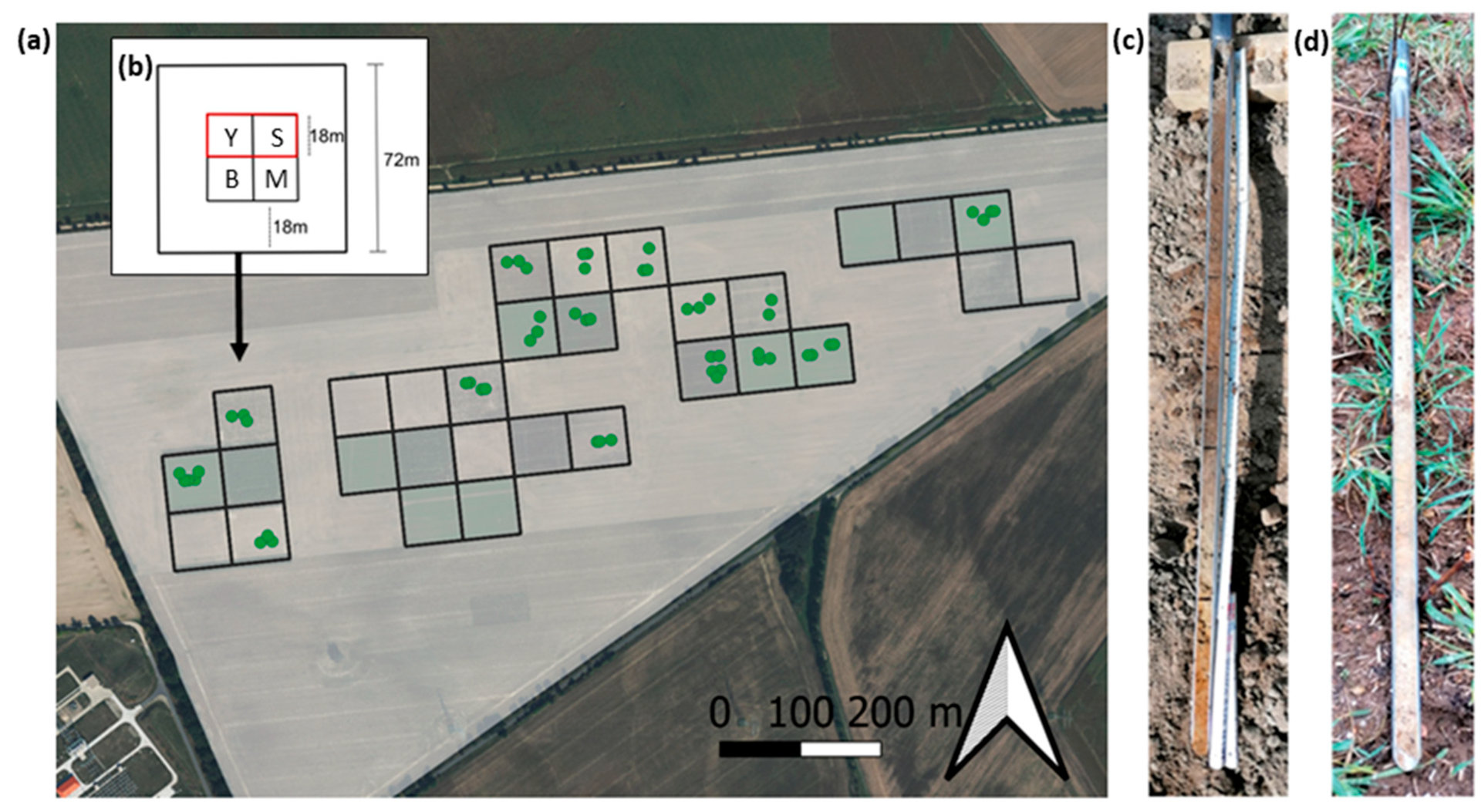
2.1. Experimental Site

Soil data collection was carried out in the 70-ha field of the patchCROP landscape laboratory. The experimental site is located in Tempelberg, east Brandenburg, Germany (52.4426° N, 14.1607° E). The area displays a characteristic undulating young moraine landscape with an elevation between 67 and 81 m.a.s.l. [32]. Spatial soil characteristics at the site vary due to past glaciation events, displaying cambisol, luvisol, and truncated luvisol soil types in the top- and subsoil layers, with loamy sand to sandy loam derived from glacial deposits. Multiple glaciation processes resulted in complex dynamics that created very heterogeneous soil textural conditions in the top- and subsoil due to the nature of the transported sediments [32,33]. Past soil formation processes result in marked crop growth and yield productivity patterns [34]. From 1980 to 2010, the average annual mean temperature at the site was 9.2 °C, while the average annual rainfall was 568 mm, ranging from 373 to 774 mm.

2.2. patchCROP Landscape Laboratory

The experiment was established in 2020 to study how diversified cropping systems in the form of new field arrangements can contribute to more multifunctional landscapes in terms of crop productivity, delivery of ESSs, and biodiversity [34]. Depending on soil characteristics, the 70 ha field was subdivided into small, homogenous ~0.5 ha sub-units called “patches” (Figure 1), which share similar soil characteristics, allowing for patch-specific management [35]. Each patch is subdivided into four central quadrants of 18 × 18 m each to ensure parameter-associated comparisons over time: one for biomass and final yield sampling, a second for soil-related sampling, a third for biodiversity-related measurements, and a multipurpose quadrant; the remaining area around the quadrants is designated as a buffer zone (Figure 1b). For more information about the experiment, refer to Grahmann et al. [34].

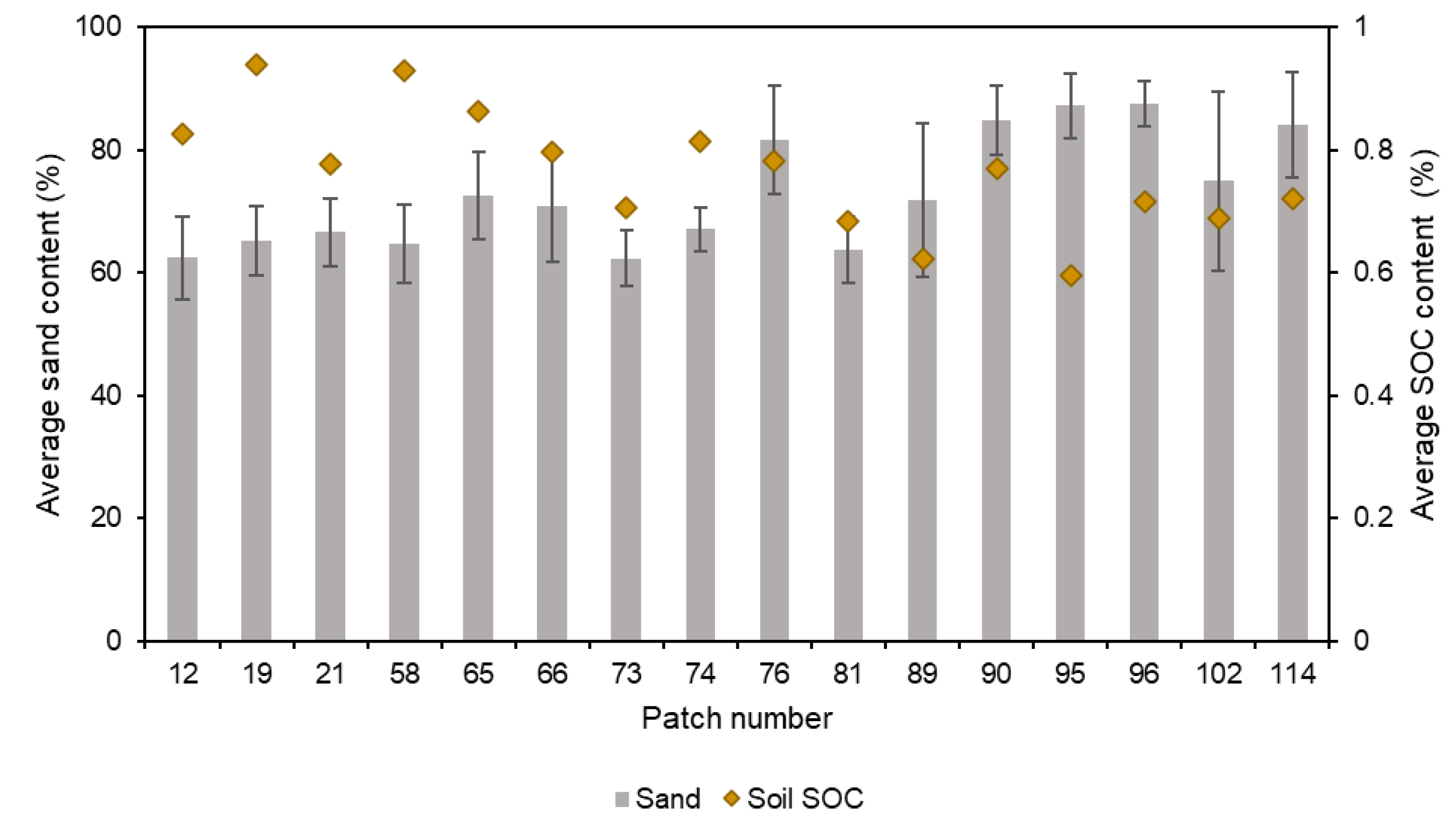
2.3. Soil Data Collection and Soil Available Water Categories

Soil samples were collected at 16 selected patches using a 1 m Pürckhauer soil auger with an 18 mm inner diameter (Figure 1 and Figure S1). The soil samples in each patch were collected by delineating two parallel transects from east to west in the soil and yield quadrant. Within a transect, each soil auger profile was 5 m apart (Figure S1). Transects in the soil quadrant were adjusted to prevent damage to the buried soil moisture sensors. Eight soil auger profile samples were collected at each quadrant, resulting in 16 sampling points per patch (Figure S1). Each soil auger profile was individually described by subdividing it into layers depending on color and density changes (Figure 1c,d). The soil color by layer was estimated using a Munsell color chart [36]. The soil textural class by layer was estimated in the field using the “Finger test to determine soil texture according to DIN 19682-2 and KA5” [37]. Soil carbonate presence was determined in the field using a 10% HCl solution directly applied to the soil [38]. Similarly, stone and mottle presence were estimated using the FAO guidelines [38]. Afterward, two to four representative soil auger profiles for the 16 recorded points within each patch were chosen for further laboratory analysis. Laboratory-based soil texture analysis by layer was performed by using the wet sieving and sedimentation method (DIN 148 ISO 11277 [39] reference method). The particle size distribution was defined according to the IUSS Working Group 150 WRB [40]. Soil pH was measured using a CaCl2 solution. Additionally, soil C/N was determined with a C/N analyzer (EuroEA3000, EuroVector S.p.A., Pavia, Italy). As all collected samples tested negative for carbonate presence, we assumed that all the measured carbon belonged to the organic portion. For the current study, only lab-analyzed soil samples were considered, resulting in 49 soil auger profiles (Figure 1a).
For these soil auger profiles, sand content varied from 60.7% to 89.4%, soil organic carbon (SOC) in the top layer was generally low at <1.0% (Figure 2) and declined in the subsoil. Similarly, total soil N in the top layer was also low, ranging from 0.05 to 0.1%. The depth of the loamy layer in the subsoil varied substantially depending on the soil profile, ranging from 30 cm to over 1 m deep. For modeling purposes, we assumed that soil characteristics up to 2 m were the same as in the last layer of the 1 m soil auger profile. The soil hydraulic properties (wilting point, field capacity, and saturation point) by layer were calculated using the Hypres function [41,42], which uses soil layer thickness, soil texture, SOC, and bulk density (BD) as input. Based on limited samples collected in previous campaigns, the BD was estimated to be 1.5 and 1.7 g cm3 in the top- and subsoil, respectively.
Cropping systems in the Brandenburg region are primarily rainfed, and the area is dominated by sandy soils, which generally results in poor water holding capacity [43]. Brandenburg is also one of the federal states that receives the least annual rainfall [44]. Consequently, the dominant limiting crop growth factor in this region is water stress [43,45]. Therefore, the soil auger profiles were classified into five equal range categories, depending on their plant available water capacity (PAWC) within the extended 2 m soil profile. This classification was based on Habib-ur-Rahman et al. [16]. The range of soil characteristics for each soil PAWC category are shown in Table 1.

2.4. Climate Data and Seasonal Rainfall Categories

The selected climate period was from 1 January 1990 to 31 December 2019. As climate data for the period of interest were not available for the experimental site, we chose a weather station nearby, at the Leibniz Centre for Agricultural Landscape Research (ZALF) in Müncheberg, which was about 8 km away from the experimental site. For the period from 1 January 1990 to 28 February 1991, no data were available at the weather station; therefore, the climate data were collected from gridded climate data at a 1 × 1 km resolution, derived from the German Weather Service (DW). Annual average temperature and rainfall data are shown in Figure 3.
We additionally categorized the cropping seasons for the winter and summer crops into four categories based on seasonal rainfall (rainfall from sowing to harvest), with 1 representing the lowest and 4 the highest seasonal rainfall (Table 2). A different seasonal rainfall classification with three categories was used for lupine, as it had the shortest growing season among all crops. The seasonal rainfall categories for winter crops were the same, but for winter wheat and barley, seasonal rainfall ranges comprised just the first three categories.

2.5. Crop Management

For the current study, eight winter and summer crops currently grown at the experimental site were selected. Summer crops included maize (Zea mays L.), soybean (Glycine max L.), lupine (Lupinus angustifolius), and sunflower (Helianthus annuus L.), while winter crops included rapeseed (Brassica napus L.), barley (Hordeum vulgare L.), wheat (Triticum aestivum L.), and rye (Secale cereale). For the model set up, crop cultivar, sowing date, and fertilizer applications were the same for every season, and they were based on the management data from 2020 to 2023 of the patchCROP landscape laboratory (Table 3). The earliest crop to be sown was lupine on 20 March, and the last crop to be sown was winter wheat on 17 October. Nitrogen (N) fertilizer was applied two to three times during the vegetative stage. All other macro- and micronutrients were applied to ensure optimum levels and avoid plant stress. Soybean and lupine did not receive N fertilizer but were inoculated with rhizobia about 24 h before sowing by using RADICIN® LUPIN (JOST GmbH, Iserlohn, Germany) for lupine in all years. As for soybean, RADICIN® SOJA (JOST GmbH, Iserlohn, Germany) was used in 2020, HiStick® Soja (BASF, Ludwigshafen, Germany) in 2021, and TURBOSOY® (SAATBAU, Leonding, Austria) in the following years. The inoculation took place indoors to avoid rhizobium exposure to UV light. Rhizobium inoculation was not used as model input, as the model does not consider these symbiotic dynamics.

2.6. Model Description

A model solution within the SIMPLACE (Scientific Impact assessment and Modelling PLatform for Advanced Crop and Ecosystem management, [46]) modeling framework was used for the current study. The framework has been widely used for cropping system analysis in over 30 crops [46]. It comprises SimComponents (i.e., a function or set of functions representing critical crop-, plant-, or soil-related processes) that, when combined, form an agroecosystem model (also called a model solution). One advantage of this framework is the versatility of exchanging SimComponents according to the user’s needs regarding research questions, complexity, and available data. For the current study, we used the <Lintul5, Slim, SoilCN> model solution [47] (see also Section 2.8 Model Performance). Simulations are carried out in a daily time step, and biomass is simulated using the radiation use efficiency concept, where potential biomass is calculated based on intercepted light, leaf area index, and extinction coefficient and then further reduced by water and N stress. We did not consider the rest of the macro- and micronutrients, as N tends to be the most limiting nutrient and because the model does not include dynamics of micronutrient availability and uptake. Then, biomass is partitioned into different organs depending on the crop developmental stage (DVS). In early developmental stages, about half of the biomass produced within a day goes to the roots, while the rest is split into the leaves and stems; as the DVS progresses, more biomass partitions into the leaves and stems. After flowering occurs, all assimilates are redirected to the storage organs. Maximum rooting depth is crop specific and is defined in the crop parameter file (Table S1); the crop uptake of water and nutrients (N in this case) occurs in the soil layers where roots are present. If no strong water or N stress occurs during the vegetative stage, the maximum rooting depth is achieved by the time of flowering. For further model details, refer to Hernandez-Ochoa et al. [47].

2.7. Model Set Up and Initial Conditions

Each crop was simulated for 30 years (1990 to 2020) for every soil auger profile. Atmospheric CO2 was set to 381 ppm, the average corresponding to the period from 1990 to 2019. The model was initialized every year 30 days before sowing to avoid carryover effects during the simulation period. Limited observations of soil mineral N indicated differences in the soil mineral N content of the patches; therefore, initial soil mineral N was set to 200 kg ha1 for the patches toward the northwest and 70 kg ha1 for the ones toward the southeast area (Figure S1d). Given the rainfall patterns in the studied area, the initial soil water content was set at 100% and 30% field capacity for the summer and winter crops, respectively.

2.8. Model Performance

The model was previously calibrated and validated using the 2020–2022 observed crop growth data from the patchCROP experiment [34], showing reasonable performance for total intermediate and final aboveground biomass growth as well as grain yield for most crops, except rye and sunflower, primarily due to intense water stress [47]. Further model testing showed reasonable model performance in reproducing the spatial patterns of soil moisture dynamics and crop growth for the studied crops [48,49]. Therefore, the model can be a reliable tool to explore the impacts of within-field heterogeneities and contribute to cropping system design for improved resource management toward enhanced system sustainability.

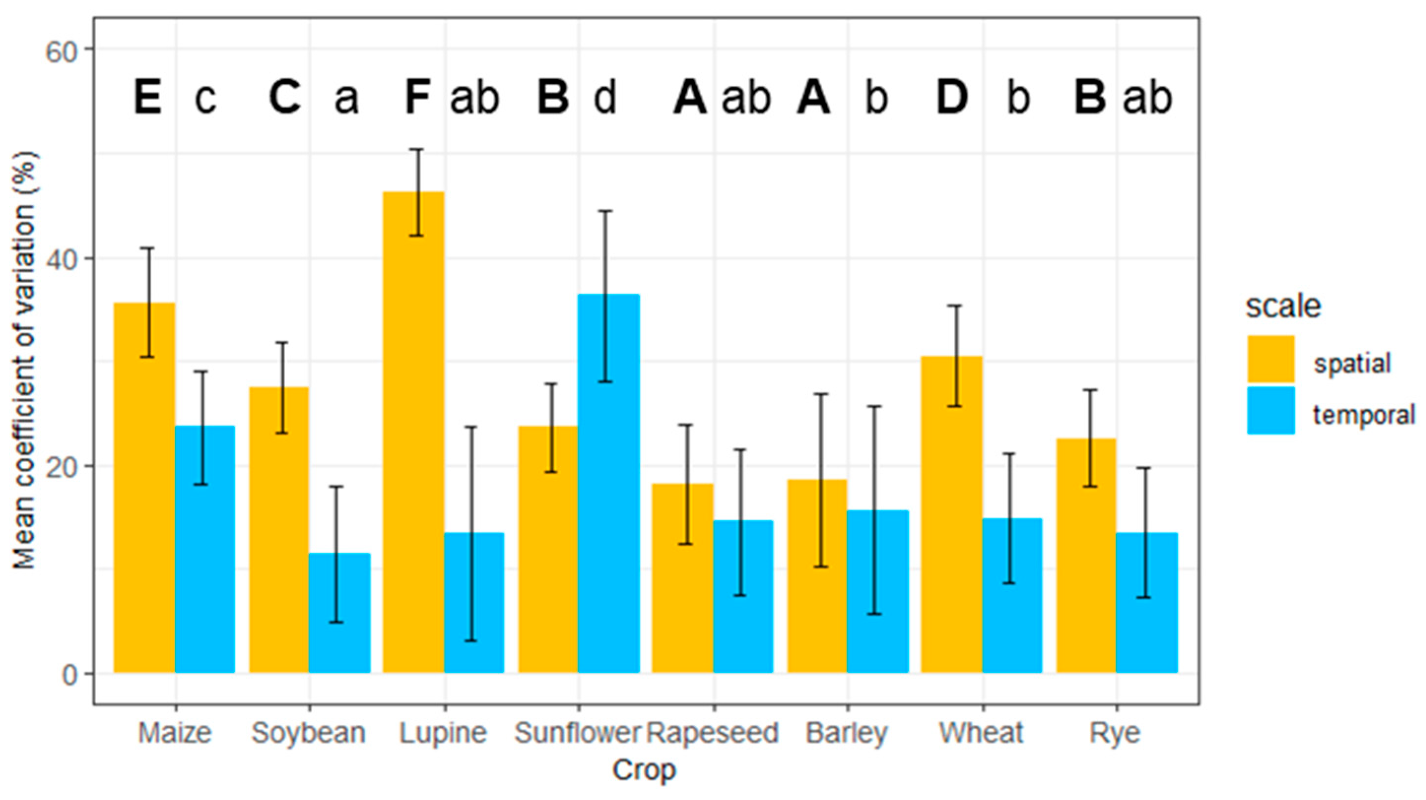
2.9. Grain Yield Spatial and Temporal Variability

The simulated spatial and temporal variation was calculated using the coefficient of variation (CV). For a particular crop, the temporal variability was calculated as the average CV for grain yields within the 30-year simulated period. In contrast, the spatial variation in each crop was calculated as the CV among all the 49 soil auger profiles.

2.10. Statistical Approach

As data were non-normally distributed, non-parametric tests were chosen for data analysis. To explore the differences among crops for temporal and spatial variation, we used a Kruskal–Wallis rank-based multiple mean comparison test using the Agricolae package in R studio; the multiple mean comparisons were performed by applying the Duncan’s multiple range test. Moreover, to explore the interaction between seasonal rainfall categories and soil characteristics (PAWC categories), an aligned ranks transformation ANOVA for factorial design [36] was used for the simulated grain yields. Then, a Tukey test (p level < 0.05) was conducted to identify treatment differences at a 0.05 probability level. The main effects and interactions were tested separately by crop. The statistical analysis was conducted using the ARTool package in R studio (Version 4.4.2).

3. Results

3.1. Simulated Grain Yield

Simulated grain yields of summer and winter crops were affected by within-field heterogeneities and climate conditions for the 30-year simulation period (Figure 4). Absolute simulated grain yields were the highest for winter crops, with barley resulting in the highest average grain yield at 6.93 t ha−1 (Figure 4). In general, summer crops produced lower grain yields than the winter crops, with maize showing the highest average simulated grain yield at 6.02 t ha−1, while legumes and sunflower resulted in the lowest average grain yield for the simulated period with <2.15 t ha−1 (Figure 4).

3.2. Simulated Grain Yield Spatial and Temporal Variability

The spatial variability tended to be higher than the temporal variability for all winter and summer crops, except for sunflower (Figure 5). The highest spatial variability (CV) among simulated crops was for lupine (45.8%) and maize (34.9%), while soybean and sunflower showed considerably lower spatial variability, with 27.0% and 23.3% CV, respectively. As for the winter crops, winter wheat showed the highest spatial variability at 29.8% CV, and thereafter, the lowest spatial variability was simulated for rapeseed and barley at about 17.4% CV. As for the temporal variability, sunflower and maize were the most variable crops, with 36.8% and 22.3% CV, respectively. In contrast, the legume crops soybean and lupine showed the lowest temporal variability with 10.4% and 11.2%, respectively (Figure 5).

3.3. Impacts of Soil Available Water and Seasonal Rainfall Category on Simulated Grain Yield

Summer and winter crop responses were affected by soil PAWC and seasonal rainfall categories (Table 4). The summer crops maize and sunflower showed a significant interaction between soil PAWC and seasonal rainfall category, while for the legume crops lupine and soybean, the interaction was non-significant (Table 4). As for winter crops, the soil PAWC and seasonal rainfall categories’ interaction was significant for all, except for wheat (Table 4).

3.4. Main Effects of Soil Available Water and Seasonal Rainfall Category on Simulated Grain Yield

For wheat, soybean, and lupine, grain yield tended to increase with increasing soil PAWC (Figure 6a). The comparison of soil PAWC categories 1 vs. 5 showed significant differences among all crops, but differences for the intermediate categories were less evident. Simulated soybean grain yield was the lowest in soil PAWC category 1 and the highest in soil PAWC category 5, with 1.95 and 2.56 t ha−1 simulated grain yield, respectively, followed by soil categories 3 and 4, with an average simulated grain yield of 2.20 t ha−1 (Figure 6a). As for lupine, soil PAWC categories 1, 2, and 3 performed the same, with grain yield ranging from 0.85 to 0.97 t ha−1, but soil PAWC category 4 and 5 led to significantly higher grain yields compared to soil PAWC category 1 at 1.05 and 1.20 t ha−1, respectively. For winter wheat, grain yield responses to soil PAWC categories 1 and 2 were not significantly different, with about 5.05 t ha−1 simulated grain yield, representing the worst-performing grain yield. The highest wheat grain yield was achieved in soil PAWC category 5 with 6.84 t ha−1, followed by soil PAWC category 4 with 6.42 t ha−1 (Figure 6a).
Regarding the seasonal rainfall categories, the lowest rainfall category always led to the lowest grain yield, but grain yield responses to increased water supply varied (Figure 6b). For instance, soybean grain yield progressively increased as the rainfall category increased from 1, with 2.31 t ha−1, to 3, with 2.56 t ha−1. However, higher rainfall supply in category 4 did not increase grain yield (Figure 6b). Lupine showed increased grain yield as seasonal rainfall increased, with grain yield increasing from 0.57 to 1.45 t ha−1 (Figure 6b). Winter wheat grain yield showed the highest response to seasonal rainfall. Grain yield consistently increased as seasonal rainfall increased, with about a 60% grain yield increase in seasonal rainfall category 3 compared to seasonal rainfall category 1 (Figure 6b).

3.5. Interactions Between Soil Available Water and Seasonal Rainfall Categories on Simulated Grain Yield

Soil PAWC category and seasonal rainfall interactions were significant for the summer crops maize and sunflower (Figure 7) and the winter crops rapeseed, barley, and rye (Figure 8). For maize, the lowest simulated grain yield was observed across soil PAWC categories when the lowest seasonal rainfall occurred. The highest seasonal rainfall, categories 3 and 4, significantly increased grain yield, with non-significant differences between them across the soil water categories (Table 4, Figure 7a). The highest simulated grain yield among all combinations was simulated in the soil PAWC category 5 with seasonal rainfall categories 3 and 4 (Figure 7a). For sunflower, grain yield was lowest in the soil PAWC category 1, even when rainfall increased up to seasonal rainfall category 3 (Figure 7b). Seasonal rainfall category 4 resulted in a significant yield increase in soil PAWC categories 1 and 5 (Figure 7b). However, grain yield response was the same across the seasonal rainfall categories for soil PAWC categories 2 and 3 (Figure 7b).
In winter crops, simulated grain yield was generally higher than in summer crops. Within-field soil heterogeneity effects were more apparent when rainfall was within the lower rainfall categories 1 to 3. In the highest seasonal rainfall categories 3 and 4, the magnitude of grain yield increase varied by crop (Figure 8). Among soil PAWC categories, rapeseed showed the lowest grain yield when rainfall was the lowest but significantly increased in seasonal rainfall category 2, followed by seasonal rainfall category 3 and 4, which resulted in further significant yield increases, with no significant differences between them, except in soil PAWC 5, where seasonal rainfall 4 showed the highest grain yield (Figure 8a). Barley was the least affected by soil heterogeneities, with the lowest grain yield simulated in soil PAWC categories 1 and 2 when the lowest seasonal rainfall occurred. In soil PAWC categories 3 and 4, simulated grain yield was the same regardless of the seasonal rainfall. Interestingly, the highest soil PAWC category and highest rainfall resulted in a reduction in barley grain yield due to nutrient leaching. For rye, grain yield significantly increased from seasonal rainfall category 1 to 2 for all the soil PAWC categories; seasonal rainfall categories 3 and 4 led to the highest grain yield across all soil PAWC categories, with no significant differences between them, except in soil PAWC category 5, where the grain yield was highest with seasonal rainfall 4 (Figure 8c).
When comparing the correlation coefficients to assess the effect of either seasonal rainfall, rainfall during the vegetative phase, rainfall during grain filling, or rainfall from the spring period (starting on 1 April) to harvest (just for winter crops) with grain yields, different patterns emerged. For summer crops, the relationships varied, with seasonal rainfall showing stronger correlation coefficients for lupine (0.80) and sunflower (0.23), while for maize, there was a stronger relationship with rainfall during the vegetative period (0.53), and for soybean, with rainfall during the grain filling period (0.42) (Table S2). However, for winter crops, total seasonal rainfall showed a stronger positive relationship with simulated grain yields, with the correlation coefficients varying from 0.23 for barley to 0.53 for rye (Table S3). The second strongest relationship was observed with rainfall from spring (1 April) until harvest, which showed a stronger positive relationship than rainfall during the vegetative or grain filling period (Table S3). Overall, simulated grain yields were more consistent under high rainfall supply, with the standard deviation being the lowest, particularly in the highest seasonal rainfall category. Low rainfall always led to detrimental grain yield across soil PAWC categories.

4. Discussion

A simulation experiment was conducted by combining detailed measured soil data from a heterogeneous field with a calibrated and validated agroecosystem model to evaluate summer and winter crop responses to heterogeneous soil conditions over a 30-year period. Simulation results showed that there was a significant effect of soil characteristics and seasonal rainfall on grain yield variability, with most crops showing an interaction between the two factors, except for soybean, lupine, and winter wheat, which showed non-significant interactions. Absolute grain yields were the highest in winter crops and maize, while legumes and sunflower showed lower yield levels under the studied soil conditions. Spatial and temporal grain yield responses varied by crop.

4.1. Simulated Grain Yield and Variability

In general, summer and winter crop yields were within the yield levels of the Oder-Spree district, where the experimental site is located (Figure S2). Among the summer crops, maize showed the highest crop productivity but also the second highest temporal variability. Our results also showed a higher correlation of maize grain yield with rainfall during the vegetative stage, which is in contrast to the report by Schillerberg et al. [50], who reported a stronger correlation of rainfall during the grain filling period than during the vegetative stage for maize. Interestingly, for about a third of the simulated seasons, soybean and maize failed to reach physiological maturity, particularly during the first and second decades of the simulations, where the observed weather exhibited a slight linear trend of increasing temperature, preventing the crops from reaching maturity due to insufficient thermal time accumulation. This condition was possibly because the modern cultivars used in the simulations were bred under higher temperature levels in the last decade, leading to higher thermal requirements for phenological development, and were not adapted to the lower temperature level at the beginning of the simulation period representing the end of the last century. In the current model setting, if soybean or maize did not reach maturity within the sowing year, the harvest was forced at the end of the year (31 December), although the simulated growth and grain filling processes stopped earlier. This likely had an influence on the relationships between grain yield and seasonal rainfall and is possibly also reflected in the lack of grain yield response between seasonal rainfall categories 2 and 3 in soybean and maize. For winter crops, seasonal rainfall and rainfall during the spring period until harvest (physiological maturity) showed the highest correlation coefficients with grain yield, suggesting that rainfall during the early growth period, even during winter, plays a significant role in yield realization, possibly due to the fact that winter crops tend to have deeper root systems that allow them to take advantage of the stored water and nutrients in deeper soil layers [51].
The rest of summer crops resulted in lower simulated grain yields. The simulated soybean yields were similar to those generally observed in the region (Figure S2, [52]). Despite the lower yields compared to those of maize, soybean can be a more desirable crop, as it has a considerably higher value than maize [53] and additionally delivers the benefits of fixing nitrogen. Research shows that legumes tend to be sensitive to water stress during both the vegetative and grain filling periods [54], as it can cause reduced emergence, photosynthesis, and nutrient uptake and thus reduced yield formation and even crop failure; similar responses are reported for sunflower [55]. Lupine also has the shortest seasonal duration, contributing to its low grain yield compared to that of other crops. Lupine showed the largest spatial variation of all crops at >40%, which suggests a higher sensitivity to soil conditions. As for sunflower, though the yield level was similar to that in Brandenburg state, sunflower performed poorly under the studied conditions, showing the largest temporal variation. However, the spatial variation in the simulated sunflower yield was similar to that in the rest of the crops, which suggested instead a higher sensitivity to seasonal weather that can result in high water stress, which was also observed under field conditions [47].
Winter crops resulted in the highest simulated grain yield, with spatial variability being more prominent than temporal variability. Winter wheat showed a higher spatial variability (30%) than the remaining winter crops (~19%). Wheat tends to be more sensitive to water stress compared to other crops like rye and barley [56], which is also reflected in crop model parameters, where water stress in wheat causes a higher percentage of dead leaves, which leads to a yield drop under water-limiting conditions. Barley was the crop with the highest grain yield, suggesting that it was least affected by water stress among the winter crops. However, reports show that rye tends to be more tolerant to water stress than barley [57]. The earlier grain filling period in barley compared to that in the other cereal winter crops may also contribute to drought escape [57]. Despite of the longer duration of the vegetative phase in all winter crops, rainfall from spring to harvest and the total seasonal rainfall showed higher correlation coefficients than rainfall during the vegetative stage. This response differs from the report of Schittenhelm [57], who suggested that rainfall during the vegetative stage had a stronger impact on biomass accumulation in cereal crops. Also, a deeper root system in winter crops may allow them to extract water from deeper soil layers under limited water supply (Table S1) [58]. Simulated grain yields showed a higher variation (standard error bars) when rainfall supply was lower, but among the years with the highest seasonal rainfall, the grain yield variation, particularly in winter crops, was the lowest, regardless of the soil PAWC capacity. This suggests that within-field heterogeneities tend to be more prominent under limited water supply than under ample water supply. These results are similar to the ones reported by Stadler et al. [18], who reported that dry weather conditions led to distinctive growth patterns in observed winter wheat and barley LAI. Kravchenko et al. [59] also reported that wheat, maize, and soybean yields showed the highest CVs under environmental stress compared to those under optimum conditions.

4.2. Main Effects and Interactions of Soil Available Water and Seasonal Rainfall Categories on Simulated Gran Yield

Most crops resulted in significant interactions between soil PAWC and seasonal rainfall, though no particular trend was observed between the summer and winter crops. Our results showed a significant interaction of soil water conditions and seasonal rainfall for the winter crops rapeseed, barley, and rye and for the summer crops maize and sunflower. Therefore, the optimization of cropping system design may be more complex, as optimal spatial and temporal crop arrangements will vary depending on the rainfall conditions. However, for wheat and legumes, simulated results suggest more consistent spatial patterns during wet and dry years, where the higher soil PAWC areas will perform better than the low soil PAWC areas, with the overall yield level depending on the rainfall conditions. Lupine performed best under the highest seasonal rainfall and/or the highest soil PAWC category but tended to be less responsive under low water soil storage capacity or seasonal rainfall. Similarly, for soybean, the crop performed equally under the two highest seasonal rainfall categories, while grain yield was significantly affected by soil PAWC. Our results also showed that simulated grain yield responses to seasonal rainfall were higher in low soil PAWC than in high soil PAWC categories. Summer crops instead were shown to be more affected by soil PAWC categories, even at high seasonal rainfall, possibly due to the shorter seasonal duration compared to that of the summer crops.
During the calibration and validation of the current agroecosystem model, we observed large errors in model performance for rye and sunflower, which may result in overestimating the simulated water stress. However, the model performed reasonably well for the other crops [47]. Further calibration and validation of soil water dynamics and aboveground biomass during flowering across multiple locations at the experimental site offer increased confidence in the results [49]. The current study shows the potential of combining detailed soil data and a previously calibrated agroecosystem model to understand the interactions between soil conditions and interannual variability in climate under rainfed systems and therefore provides meaningful information that can serve for cropping system design. The results also showed that the simulated yield responses to soil and weather variability differed between summer and winter crops. Under the studied conditions, there was also a strong pattern of field heterogeneities, typical of landscapes influenced by past glacial activities. Therefore, there may be potential to use this data to optimize the spatial distribution of crops. The management of small-scale diversified cropping systems may become more feasible in the future with the development of more miniature robots that may allow for the management of smaller field sizes for multifunctional agroecosystems that promote the delivery of ESSs with reduced environmental impacts while also promoting biodiversity and increasing resilience to climate change. Additionally, seasonal weather forecasts may contribute to improved cropping system design. When water is limited, there is potential to reduce crop yield loss by increasing crop diversification, allocating crops according to their tolerance to water stress, and adjusting nitrogen application rates to optimize crop uptake and reduce nutrient losses. For summer crops such as lupine and sunflower, which showed strong simulated water stress, breeding efforts focused on water stress tolerance can be beneficial [60]. Other management strategies that preserve soil moisture (such as conservation agriculture) or provide support to avoid stress (such as a change in sowing dates) can also contribute to improved crop adaptation under water-limiting conditions [55].

5. Conclusions

The highly variable soil water holding capacity and the low seasonal rainfall in the studied region in the state of Brandenburg compared to other parts of Germany makes rainfed crops particularly vulnerable to environmental conditions. This study provides valuable information about the temporal variability in crop productivity for a range of crops and about the impacts of within-field soil heterogeneities. The correlations between total seasonal rainfall, rainfall during the vegetative period, and rainfall during grain filling varied according to crop. Winter crop yield for most crops showed an interaction between soil and seasonal rainfall conditions, except for wheat. However, for summer crops, no clear trend was observed; the greater spatial variability in yields suggests a higher sensitivity to soil conditions despite rainfall supply. Strong within-field variability in crop yield shows the potential to develop strategies to manage and allocate resources according to crop productivity. Given sufficiently detailed data, this methodology can also be applied to other regions to increase crop diversification and better understand and quantify the synergies and trade-offs of diversified cropping systems in terms of crop productivity, the delivery of ESSs, and resource use, which may provide more insights into the crop interactive effects of soil and climate conditions on grain yields.

Supplementary Materials

The following supporting information can be downloaded at: https://www.mdpi.com/article/10.3390/agronomy15030661/s1, Table S1: Crop maximum rooting depth for the 30-year simulations.; Table S2: Correlation coefficients for summer crops for seasonal rainfall (Seasonal rain), rainfall during the vegetative period (RainVeg), and rainfall during the rainfall period (RainGF) with simulated grain yield; Table S3: Correlation coefficients for winter crops for seasonal rainfall (SeasonalRain), rainfall during the vegetative period (RainVeg), rainfall during the rainfall period (RainGF), and rainfall from April 1st to maturity (RainSpringToMat) with simulated grain yield at the patchCROP landscape experiment, Brandenburg, Germany; Figure S1: Exemplary transects for the soil sampling campaign conducted at the patchCROP landscape laboratory for patches (a) 12, 21, 58, 65, 74, 76, 89, 96, 102, 114, (b) 66, 73, 81, 90, 95, and (c) 19. (d) Initial soil mineral N for green and purple patches was set to 200 and 70 kg ha−1, respectively. Two transects from east to west were delineated. Transects in the yield quadrant were 10 m apart, with a 4 m equal distance from the quadrant border. Transects in the soil quadrant were 8 m apart to avoid buried sensor damage. Eight soil auger profile samples, each 5 m apart, were collected in each quadrant, resulting in a total of 16 per patch; Figure S2: Average (2010–2020) observed and simulated grain yield for summer and winter crops. Observations correspond to seasonal data for the Oder Spree district, Brandenburg, where the experimental site is located, in the state of Brandenburg Germany. Simulated grain yield corresponds to the average of the 49 soil auger profiles for the patchCROP landscape laboratory field. Observations extracted from the Berlin-Brandenburg Office for Statistics [38]. Observed grain yield data for soybean not available. Observed maize yield corresponds to “grain corn/corn for ripening (including corn cob mix)”. Observed rye yield is reported together with winter meslin. Observed wheat yield from 2010 to 2016 comprised both spring and winter seasons; grain yield from 2017 to 2020 corresponds to winter wheat, including spelt and einkorn.

Author Contributions

Conceptualization, I.M.H.-O., T.G. and F.E.; methodology, I.M.H.-O., T.G. and F.E.; formal analysis, I.M.H.-O.; writing—original draft preparation, I.M.H.-O.; writing—review and editing I.M.H.-O., T.G., F.E., K.G. and A.M.E.; visualization, I.M.H.-O. and A.M.E.; supervision, T.G. and F.E. All authors have read and agreed to the published version of the manuscript.

Funding

This work was supported by the Deutsche Forschungsgemeinschaft (DFG, German Research Foundation) under Germany’s Excellence Strategy—EXC 2070—390732324. This work was additionally supported by the BMBF for the Junior Research Group SoilRob, project ID 031B1391. The maintenance of the patchCROP infrastructure is supported by the Leibniz Centre for Agricultural Landscape Research.

Data Availability Statement

Soil data, model solutions, and simulated data can be made available upon request.

Acknowledgments

Special thanks to G. Krauss for his technical support.

Conflicts of Interest

The authors declare no conflicts of interest.

Abbreviations

The following abbreviations are used in this manuscript:
ESSEcosystem service
PAWCPlant available water capacity
LAILeaf area index
G × M × EGenotype × management × environment
m.a.s.l.Meters above sea level
NNitrogen
SOCSoil organic carbon
ZALFLeibniz Centre for Agricultural Landscape Research

References

  1. FAO; IFAD; UNICEF; WFP; WHO. The State of Food Security and Nutrition in the World 2020. Transforming Food Systems for Affordable Healthy Diets; Food & Agriculture Organization: Rome, Italy, 2020; p. 320. [Google Scholar]
  2. Ewert, F.; Baatz, R.; Finger, R. Agroecology for a sustainable agriculture and food system: From local solutions to large-scale adoption. Annu. Rev. Resour. Econ. 2023, 15, 351–381. [Google Scholar] [CrossRef]
  3. Pretty, J.; Benton, T.; Bharucha, Z.; Dicks, L.; Flora, C.; Godfray, H.; Goulson, D.; Hartley, S.; Lampkin, N.; Morris, C.; et al. Global assessment of agricultural system redesign for sustainable intensification. Nat. Sustain. 2018, 1, 441–446. [Google Scholar] [CrossRef]
  4. IPCC. Fact Sheet Europe, Climate Change Impacts and Risks. 2022. Available online: https://www.ipcc.ch/report/ar6/wg2/downloads/outreach/IPCC_AR6_WGII_FactSheet_Europe.pdf (accessed on 13 August 2024).
  5. Godfray, H. The debate over sustainable intensification. Food Secur. 2015, 7, 199–208. [Google Scholar] [CrossRef]
  6. Kamau, H.; Roman, S.; Biber-Freudenberger, L. Nearly half of the world is suitable for diversified farming for sustainable intensification. Commun. Earth Environ. 2023, 4, 446. [Google Scholar] [CrossRef]
  7. Cassman, K.; Grassini, P. A global perspective on sustainable intensification research. Nat. Sustain. 2020, 3, 262–268. [Google Scholar] [CrossRef]
  8. Beillouin, D.; Ben-Ari, T.; Malezieux, E.; Seufert, V.; Makowski, D. Positive but variable effects of crop diversification on biodiversity and ecosystem services. Glob. Change Biol. 2021, 27, 4697–4710. [Google Scholar] [CrossRef]
  9. Hufnagel, J.; Reckling, M.; Ewert, F. Diverse approaches to crop diversification in agricultural research. A review. Agron. Sustain. Dev. 2020, 40, 17. [Google Scholar] [CrossRef]
  10. Hernandez-Ochoa, I.M.; Gaiser, T.; Kersebaum, K.C.; Webber, H.; Seidel, S.J.; Grahmann, K.; Ewert, F. Model-based design of crop diversification through new field arrangements in spatially heterogeneous landscapes. A review. Agron. Sustain. Dev. 2022, 42, 74. [Google Scholar] [CrossRef]
  11. Maestrini, B.; Basso, B. Drivers of within-field spatial and temporal variability of crop yield across the US Midwest. Sci. Rep. 2018, 8, 14833. [Google Scholar] [CrossRef]
  12. Thompson, L.J.; Archontoulis, S.V.; Puntel, L.A. Simulating within-field spatial and temporal corn yield response to nitrogen with APSIM model. Precis. Agric. 2024, 25, 2421–2446. [Google Scholar] [CrossRef]
  13. Kersebaum, K.C.; Wallor, E. Process-based modelling of soil–crop Interactions for site-specific decision support in crop management. In Precision Agriculture: Modelling; Cammarano, D., van Evert, F.K., Kempenaar, C., Eds.; Springer: Cham, Switzerland, 2023; pp. 25–47. [Google Scholar] [CrossRef]
  14. Mulla, D.J.; Schepers, J.S. Key processes and properties for site-specific soil and crop management. In the State of Site Specific Management for Agriculture; ACSESS Publications; Wiley: Hoboken, NJ, USA, 1997; p. 18. [Google Scholar] [CrossRef]
  15. Basso, B.; Dumont, B.; Maestrini, B.; Shcherbak, I.; Robertson, G.P.; Porter, J.R.; Smith, P.; Paustian, K.; Grace, P.R.; Asseng, S.; et al. Soil organic carbon and nitrogen feedbacks on crop yields under climate change. Agric. Environ. Lett. 2018, 3, 5. [Google Scholar] [CrossRef]
  16. Habib-ur-Rahman, M.; Raza, A.; Ahrends, H.E.; Huging, H.; Gaiser, T. Impact of in-field soil heterogeneity on biomass and yield of winter triticale in an intensively cropped hummocky landscape under temperate climate conditions. Precis. Agric. 2022, 23, 912–938. [Google Scholar] [CrossRef]
  17. Falco, N.; Wainwright, H.M.; Dafflon, B.; Ulrich, C.; Soom, F.; Peterson, J.E.; Brown, J.B.; Schaettle, K.B.; Williamson, M.; Cothren, J.D.; et al. Influence of soil heterogeneity on soybean plant development and crop yield evaluated using time-series of UAV and ground-based geophysical imagery. Sci. Rep. 2021, 11, 7046. [Google Scholar] [CrossRef] [PubMed]
  18. Stadler, A.; Rudolph, S.; Kupisch, M.; Langensiepen, M.; van der Kruk, J.; Ewert, F. Quantifying the effects of soil variability on crop growth using apparent soil electrical conductivity measurements. Eur. J. Agron. 2015, 64, 8–20. [Google Scholar] [CrossRef]
  19. Wendroth, O.; Pohl, W.; Koszinski, S.; Rogasik, H.; Ritsema, C.; Nielsen, D. Spatio-temporal patterns and covariance structures of soil water status in two northeast German field sites. J. Hydrol. 1999, 215, 38–58. [Google Scholar] [CrossRef]
  20. Kersebaum, K.C.; Lorenz, K.; Reuter, H.I.; Schwarz, J.; Wegehenkel, M.; Wendroth, O. Operational use of agro-meteorological data and GIS to derive site specific nitrogen fertilizer recommendations based on the simulation of soil and crop growth processes. Phys. Chem. Earth 2005, 30, 59–67. [Google Scholar] [CrossRef]
  21. Xia, H.; Yuan, S.F.; Prishchepov, A.V. Spatial-temporal heterogeneity of ecosystem service interactions and their social-ecological drivers: Implications for spatial planning and management. Resour. Conserv. Recycl. 2023, 189, 106767. [Google Scholar] [CrossRef]
  22. Usowicz, B.; Lipiec, J. Spatial variability of soil properties and cereal yield in a cultivated field on sandy soil. Soil Tillage Res. 2017, 174, 241–250. [Google Scholar] [CrossRef]
  23. Mzuku, M.; Khosla, R.; Reich, R.; Inman, D.; Smith, F.; MacDonald, L. Spatial variability of measured soil properties across site-specific management zones. Soil Sci. Soc. Am. J. 2005, 69, 1572–1579. [Google Scholar] [CrossRef]
  24. Malezieux, E.; Crozat, Y.; Dupraz, C.; Laurans, M.; Makowski, D.; Ozier-Lafontaine, H.; Rapidel, B.; de Tourdonnet, S.; Valantin-Morison, M. Mixing plant species in cropping systems: Concepts, tools and models. A review. Agron. Sustain. Dev. 2009, 29, 43–62. [Google Scholar] [CrossRef]
  25. Asseng, S.; Zhu, Y.; Wang, E.; Zhang, W. Crop modeling for climate change impact and adaptation. In Crop Physiology; Academic Press: Cambridge, MA, USA, 2014; pp. 505–546. [Google Scholar]
  26. Ewert, F.; Rötter, R.P.; Bindi, M.; Webber, H.; Trnka, M.; Kersebaum, K.C.; Olesen, J.E.; Van Ittersum, M.K.; Janssen, S.; Rivington, M.; et al. Crop modelling for integrated assessment of risk to food production from climate change. Environ. Model. Softw. 2014, 72, 287–303. [Google Scholar] [CrossRef]
  27. Teixeira, E.; Zhao, G.; de Ruiter, J.; Brown, H.; Ausseil, A.; Meenken, E.; Ewert, F. The interactions between genotype, management and environment in regional crop modelling. Eur. J. Agron. 2017, 88, 106–115. [Google Scholar] [CrossRef]
  28. Basso, B.; Cammarano, D.; Chen, D.; Cafiero, G.; Amato, M.; Bitella, G.; Rossi, R.; Basso, F. Landscape position and precipitation effects on spatial variability of wheat yield and grain protein in Southern Italy. J. Agron. Crop Sci. 2009, 195, 301–312. [Google Scholar] [CrossRef]
  29. Jeuffroy, M.; Casadebaig, P.; Debaeke, P.; Loyce, C.; Meynard, J. Agronomic model uses to predict cultivar performance in various environments and cropping systems. A review. Agron. Sustain. Dev. 2014, 34, 121–137. [Google Scholar] [CrossRef]
  30. Leo, S.; Migliorati, M.; Nguyen, T.; Grace, P. Combining remote sensing-derived management zones and an auto-calibrated crop simulation model to determine optimal nitrogen fertilizer rates. Agric. Syst. 2023, 205, 103559. [Google Scholar] [CrossRef]
  31. Padovan, G.; Martre, P.; Semenov, M.; Masoni, A.; Bregaglio, S.; Ventrella, D.; Lorite, I.; Santos, C.; Bindi, M.; Ferrise, R.; et al. Understanding effects of genotype x environment x sowing window interactions for durum wheat in the Mediterranean basin. Field Crops Res. 2020, 259, 107969. [Google Scholar] [CrossRef]
  32. Koch, T.; Deumlich, D.; Chifflard, P.; Panten, K.; Grahmann, K. Using model simulation to evaluate soil loss potential in diversified agricultural landscapes. Eur. J. Soil Sci. 2023, 74, e13332. [Google Scholar] [CrossRef]
  33. Öttl, L.K.; Wilken, F.; Auerswald, K.; Sommer, M.; Wehrhan, M.; Fiener, P. Tillage erosion as an important driver of in-field biomass patterns in an intensively used hummocky landscape. Land Degrad. Dev. 2021, 32, 3077–3091. [Google Scholar] [CrossRef]
  34. Grahmann, K.; Reckling, M.; Hernández-Ochoa, I.; Donat, M.; Bellingrath-Kimura, S.; Ewert, F. Co-designing a landscape experiment to investigate diversified cropping systems. Agric. Syst. 2024, 217, 103950. [Google Scholar] [CrossRef]
  35. Donat, M.; Geistert, J.; Grahmann, K.; Bloch, R.; Bellingrath-Kimura, S. Patch cropping- a new methodological approach to determine new field arrangements that increase the multifunctionality of agricultural landscapes. Comput. Electron. Agric. 2022, 197, 106894. [Google Scholar] [CrossRef]
  36. Pendleton, R.L.; Nickerson, D. Soil colors and special Munsell soil color charts. Soil Sci. 1954, 71, 35–44. [Google Scholar] [CrossRef]
  37. Eckelmann, W.; Sponagel, H.; Grottenthaler, W.; Hartmann, K.J.; Hartwich, R.; Janetzko, P.; Joisten, H.; Kühn, D.; Sabel, K.J.; Traidl, R. Bodenkundliche Kartieranleitung, KA5; Federal Institute for Geosciences: Hannover, Germany, 2005. [Google Scholar]
  38. FAO. Guidelines for Soil Description; Food and Agriculture Organization of the United Nations: Rome, Italy, 2006; p. 109. [Google Scholar]
  39. ISO 11277:2002; Soil Quality—Determination of Particle Size Distribution in Mineral Soil Material—Method by Sieving and Sedimentation (ISO 11277:1998 + ISO 11277:1998 Corrigendum 1:2002). DIN: Berlin, Germany, 2002.
  40. WRB. International soil classification system for naming soils and creating legends for soil maps, IUSS Working Group WRB. In World Soil Resources Reports No. 106; FAO: Rome, Italy, 2015. [Google Scholar]
  41. Wosten, J.H.M.; Lilly, A.; Nemes, A.; Le Bas, C. Development and use of a database of hydraulic properties of European soils. Geoderma 1999, 90, 169–185. [Google Scholar] [CrossRef]
  42. Wosten, J.H.M.; Pachepsky, Y.A.; Rawls, W.J. Pedotransfer functions: Bridging the gap between available basic soil data and missing soil hydraulic characteristics. J. Hydrol. 2001, 251, 123–150. [Google Scholar] [CrossRef]
  43. Mirschel, W.; Weiland, E.; Luzi, K.; Groth, K. Model-based estimation of irrigation water demand for different agricultural crops under climate change, presented for the federal state of Brandenburg, Germany. In Landscape Modelling and Decision Support; Wilfried, M., Terleev, V.V., Wenkel, K.O., Eds.; Springer: Cham, Switzerland, 2020. [Google Scholar] [CrossRef]
  44. Wetterdienst, D. Precipitation in Germany in 2024, by Federal State (in Liters per Square Meter)-Graph. 2024. Available online: https://www.statista.com/statistics/982669/precipitation-federal-states-germany/ (accessed on 3 February 2025).
  45. von Czettritz, H.J.; Hosseini-Yekani, S.A.; Schuler, J.; Kersebaum, K.C.; Zander, P. Adapting cropping patterns to climate change: Risk management effectiveness of diversification and irrigation in Brandenburg (Germany). Agriculture 2023, 13, 1740. [Google Scholar] [CrossRef]
  46. Enders, A.; Vianna, M.; Gaiser, T.; Krauss, G.; Webber, H.; Srivastava, A.K.; Seidel, S.J.; Tewes, A.; Rezaei, E.E.; Ewert, F. SIMPLACE-a versatile modelling and simulation framework for sustainable crops and agroecosystems. Silico Plants 2023, 5, diad006. [Google Scholar] [CrossRef]
  47. Hernandez-Ochoa, I.M.; Gaiser, T.; Grahmann, K.; Engels, A.; Kersebaum, K.C.; Seidel, S.; Ewert, T. Cross model validation for a diversified cropping system. Eur. J. Agron. 2024, 157, 127181. [Google Scholar] [CrossRef]
  48. Engels, A.; Gaiser, T.; Ewert, F.; Grahmann, K.; Hernandez-Ochoa, I.M. Calibrating and validating soil moisture simulation under heterogeneous soil conditions in a diversified cropping system. In Proceedings of the Congress of the European Society of Agronomy, Rennes, France, 26–30 August 2024. [Google Scholar]
  49. Engels, A.; Gaiser, T.; Ewert, F.; Grahmann, K.; Hernandez-Ochoa, I.M. Simulating soil moisture dynamics in a diversified cropping system under heterogeneous soil conditions. MDPI Agron. 2025, 15, 407. [Google Scholar] [CrossRef]
  50. Schillerberg, T.; Tian, D.; Miao, R. Spatiotemporal patterns of maize and winter wheat yields in the United States: Predictability and impact from climate oscillations. Agric. For. Meteorol. 2019, 275, 208–222. [Google Scholar] [CrossRef]
  51. Statistik. Archive: Statistical Report, Harvest Reporting on Field Crops and Grassland (Final Result) in the State of Brandenburg (C II 2-j). 2024. Available online: https://www.statistik-berlin-brandenburg.de/archiv/c-ii-2-j (accessed on 17 January 2025).
  52. Commision, E. Agri-Food Data Portal. 2025. Available online: https://agridata.ec.europa.eu/extensions/DataPortal/home.html (accessed on 16 January 2025).
  53. Nadeem, M.; Li, J.; Yahya, M.; Sher, A.; Ma, C.; Wang, X.; Qiu, L. Research progress and perspective on drought stress in legumes: A review. Int. J. Mol. Sci. 2019, 20, 2541. [Google Scholar] [CrossRef]
  54. Ali, A.A.; Lamlom, S.F.; El-Sorady, G.A.; Elmahdy, A.M.; Abd Elghany, S.H.; Usman, M.; Alamri, A.; Shaghaleh, H.; Hamoud, Y.A.; Abdelghany, A.M. Boosting resilience and yields in water-stressed sunflower through coordinated irrigation scheduling and silica gel applications. Helyion 2024, 10, e38129. [Google Scholar] [CrossRef]
  55. Ullah, A.; Farooq, M. The challenge of drought stress for grain legumes and options for improvement. Arch. Agron. Soil Sci. 2022, 68, 1601–1618. [Google Scholar] [CrossRef]
  56. López-Castañeda, C.; Richards, R. Variation in temperate cereals in rain-fed environments I. Grain-yield, biomass and agronomic characteristics. Field Crops Res. 1994, 37, 51–62. [Google Scholar] [CrossRef]
  57. Schittenhelm, S.; Kraft, M.; Wittich, K. Performance of winter cereals grown on field-stored soil moisture only. Eur. J. Agron. 2014, 52, 247–258. [Google Scholar] [CrossRef]
  58. Odone, A.; Popovic, O.; Thorup-Kristensen, K. Deep roots: Implications for nitrogen uptake and drought tolerance among winter wheat cultivars. Plant Soil 2024, 500, 13–32. [Google Scholar] [CrossRef]
  59. Kravchenko, A.; Robertson, G.; Thelen, K.; Harwood, R. Management, topographical, and weather effects on spatial variability of crop grain yields. Agron. J. 2005, 97, 514–523. [Google Scholar] [CrossRef]
  60. Ye, H.; Roorkiwal, M.; Valliyodan, B.; Zhou, L.; Chen, P.; Varshney, R.; Nguyen, H. Genetic diversity of root system architecture in response to drought stress in grain legumes. J. Exp. Bot. 2018, 69, 3267–3277. [Google Scholar] [CrossRef]
Figure 1. (a) Selected soil sample locations at the patchCROP landscape laboratory (green dots); (b) patch quadrants (Y = biomass and yield-related sampling, S = soil-related sampling, B = biodiversity-related sampling and, M = multipurpose quadrant; sampled quadrants with red border) and buffer areas around the quadrants. Representative 1 m soil auger profiles with (c) sandy layers on top and a loamy layer at the bottom and (d) a fully sandy soil auger profile. See Figure S1 for the full soil sampling strategy.
Agronomy 15 00661 g001
Figure 2. Average sand content in the extended 2 m profile (bars) and soil organic carbon (SOC) content (diamonds) in the top layer for the sampled patches at the patchCROP landscape laboratory in Tempelberg, Brandenburg, Germany. Error bars correspond to the standard deviation of sand content for the soil samples within a patch.
Agronomy 15 00661 g002
Figure 3. Observed annual precipitation (mm) and average (Tmean), minimum (Tmin), and maximum (Tmax) temperature (°C) for a weather station in Müncheberg, close to the experimental site.
Agronomy 15 00661 g003
Figure 4. Average simulated grain yield for summer (light blue) and winter crops (dark gray) for the period from 1990 to 2020 at the patchCROP landscape laboratory in Tempelberg, Brandenburg, Germany. The red dot indicates the mean; box lines from bottom to top represent the 25th, median, and 75th percentiles. The upper and lower whiskers extend from the hinge to the largest and smallest values within the 1.5 × interquartile range, respectively. Black dots indicate outliers.
Agronomy 15 00661 g004
Figure 5. Temporal (30 years) and spatial (49 soil auger profiles) variability in grain yield for summer and winter crops at the patchCROP landscape laboratory in Tempelberg, Brandenburg, Germany. Error bars denote the standard deviation for the coefficient of variation among the years (temporal) or among the soil auger profiles (spatial). Uppercase (bold) and lowercase letters indicate mean comparisons using the Kruskal–Wallis and Duncan non-parametric tests (p < 0.05) for spatial and temporal variability among crops, respectively.
Agronomy 15 00661 g005
Figure 6. Average (1990–2020) simulated grain yield for wheat, soybean, and lupine by (a) soil plant available water capacity (PAWC, Table 1) category and by (b) seasonal rainfall water category (Table 2) when the soil PAWC and seasonal rainfall interaction effect was non-significant (Table 4). Treatments followed by the same letter are not significantly different according to the Tukey test, p value < 0.05. Mean comparisons were performed separately for each crop by comparing either the soil water categories (a) or the seasonal rainfall categories (b). The red dot indicates the mean; box lines from bottom to top represent the 25th, median, and 75th percentiles. The upper and lower whiskers extend from the hinge to the largest and smallest values within the 1.5 × interquartile range, respectively. Black dots indicate outliers.
Agronomy 15 00661 g006
Figure 7. Average (1990–2020) simulated grain yields and standard deviation for the summer crops (a) maize and (b) sunflower by soil plant available water capacity (PAWC, Table 1) category and seasonal rainfall water category (Table 2) when the two-factor interaction was significant (Table 4). Means labeled with capital letters correspond to the comparison of soil water categories within each seasonal rainfall category. Means labeled with lowercase letters correspond to the comparison of rainfall categories within each soil water category. Means followed by the same letter are not significantly different according to the Tukey test (p < 0.05). Mean comparisons were conducted separately for each crop.
Agronomy 15 00661 g007
Figure 8. Average (1990–2020) simulated grain yields and standard deviation for the winter crops (a) rapeseed, (b) barley, and (c) rye by soil plant available water capacity (PAWC, Table 1) category and seasonal rainfall category (Table 2) when the two-factor interaction was significant (Table 4). Means labeled with capital letters correspond to the comparison of soil water categories within each seasonal rainfall category. Means labeled with lowercase letters correspond to the comparison of rainfall categories within each soil water category. Means followed by the same letter are not significantly different according to the Tukey test (p < 0.05). Mean comparisons were conducted separately for each crop.
Agronomy 15 00661 g008
Table 1. Ranges of soil plant available water capacity (PAWC), sand, clay, and soil organic carbon (SOC) content for the five soil water categories for the extended 2 m soil auger profiles collected at the patchCROP landscape laboratory in Tempelberg, Brandenburg, Germany.
Soil Water CategoryNo. of ProfilesSoil PAWC
(cm 2m−1)
Average Clay Content (%)Average Sand Content (%)Top SOC (%)
189.57–12.052.93–5.3384.73–89.390.49–0.81
2512.051–14.524.40–7.8376.60–87.370.62–0.80
3414.521–17.006.23–7.6375.37–84.370.64–0.84
4717.001–19.486.55–14.2366.27–79.700.58–1.09
52519.481–21.957.17–15.7060.73–68.170.60–1.11
Table 2. Seasonal rainfall categories for summer and winter crops at the patchCROP landscape laboratory in Tempelberg, Brandenburg, Germany.
Crop/CategorySeasonal Rainfall Range (mm)
Maize, soybean, sunflower
1100–200
2200–300
3300–400
4>400
Lupine
150–150
2150–250
3250–400
Winter crops
1250–350
2350–450
3450–550
4>550
Table 3. Selected crop cultivar, sowing dates, and fertilizer application dates and amounts for summer and winter crops at the patchCROP landscape laboratory, Tempelberg, Brandenburg.
CropCultivarSowing Date
(dd/mm)
N Fertilization
Date (dd/mm)
N Fertilizer Amount
(kg ha−1)
Grain maizeP832916/0426/05100.0
26/0640.0
SoybeanAcardia30/04--
LupineBoragine28/03--
SunflowerSea bird08/0405/0420.0
16/0442.6
Rapeseed Ambassador29/0829/0850.0
07/0350.0
25/0342.5
BarleyWallace20/0910/0365.4
05/0454.0
09/0544.2
WheatUniversum17/1012/0365.4
01/0454.0
13/0544.2
RyeTayo20/0907/0342.5
05/0470.0
Table 4. Aligned ranks transformation analysis of variance p values for the effect of soil plant available water capacity (PAWC) and seasonal rainfall categories and their interaction on simulated grain yield from 1990 to 2020 for summer and winter crops at the patchCROP landscape laboratory in Tempelberg, Brandenburg, Germany.
CropsSoil PAWC
Category
Seasonal Rainfall CategorySeasonal Rainfall Category × Soil PAWC Category Interaction
Rapeseed< 2.22 × 10⁻¹⁶*** 1< 2.22 × 10⁻¹⁶*** 6.24 × 10⁻¹⁰***
Barley< 2.22 × 10⁻¹⁶*** 2.12 × 10⁻¹²***< 2.22 × 10⁻¹⁶***
Wheat< 2.00 × 10⁻¹⁶***< 2.00 × 10⁻¹⁶*** 0.74591NS
Rye< 2.00 × 10-−16***< 2.00 × 10⁻¹⁶*** 0.045239*
Maize< 2.22 × 10⁻¹⁶***< 2.22 × 10⁻¹⁶*** 0.008198**
Soybean< 2.00 × 10⁻¹⁶***< 2.00 × 10⁻¹⁶*** 0.68674NS
Lupine< 2.00 × 10⁻¹⁶***< 2.00 × 10⁻¹⁶*** 0.80205NS
Sunflower< 2.22 × 10⁻¹⁶***< 2.22 × 10⁻¹⁶***< 2.22 × 10⁻¹⁶***
1 p significance levels: 0 to 0.001 = ***; 0.001 to 0.01 = **; 0.01 to 0.05 = *; >0.05 to 1 = non-significant (NS).
Disclaimer/Publisher’s Note: The statements, opinions and data contained in all publications are solely those of the individual author(s) and contributor(s) and not of MDPI and/or the editor(s). MDPI and/or the editor(s) disclaim responsibility for any injury to people or property resulting from any ideas, methods, instructions or products referred to in the content.

