

Using High-Resolution Multispectral Data to Evaluate In-Season Cotton Growth Parameters and End-of-the-Season Cotton Fiber Yield and Quality

 , , , , , and
Abstract
1. Introduction
2. Materials and Methods
2.1. Study Site and Treatments
2.1.1. Irrigation Scheduling
2.1.2. Weather Conditions
2.2. Ground Data Collection
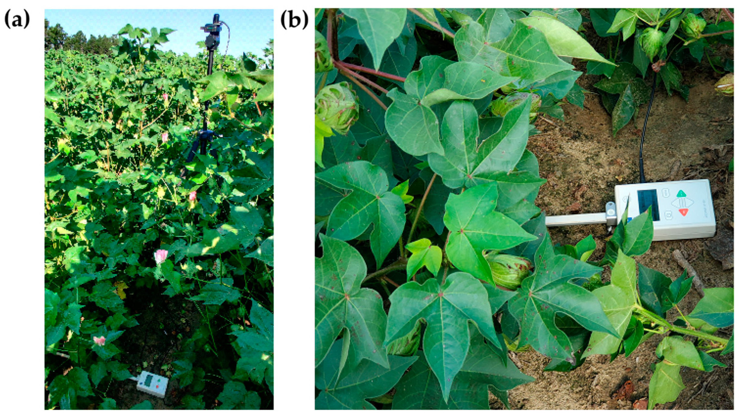
2.2.1. In-Season Measurements
2.2.2. End-of-the-Season Measurements
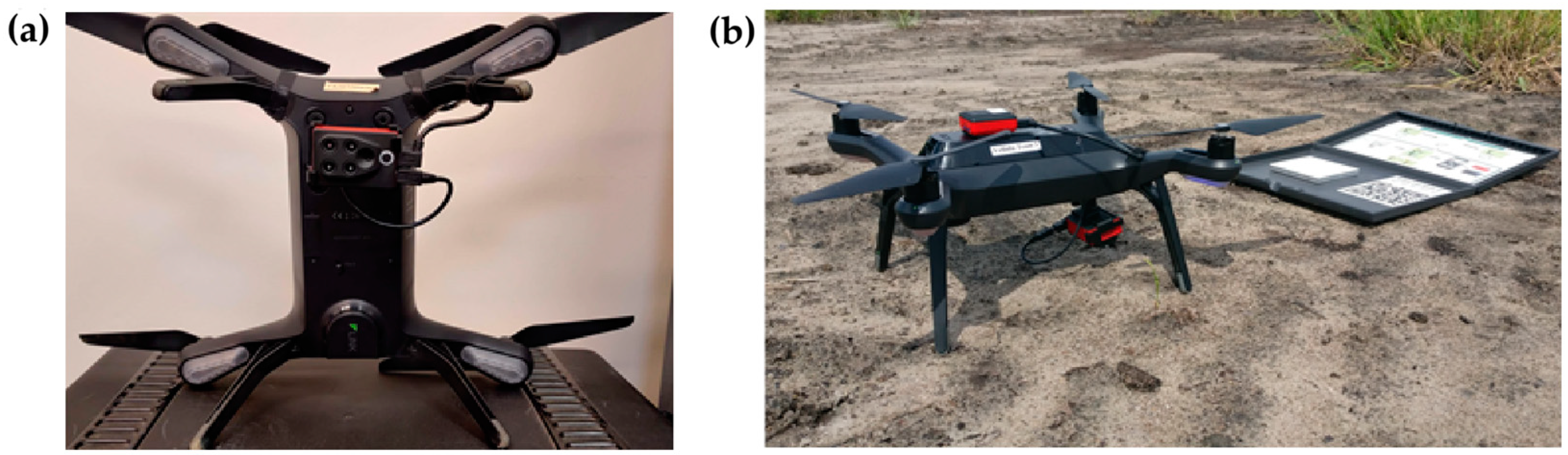
2.3. Aerial Data Collection
UAV Image Processing and Vegetation Indices (VIs) Calculation

| Vegetation Indices | Formula | Reference |
|---|---|---|
| CIRE (Chlorophyll Index Red Edge) | [37] | |
| DVI (Difference Vegetation Index) | [38] | |
| NDRE (Normalized Difference Red Edge Index) | [39] | |
| GNDVI (Green Normalized Difference Vegetation Index) | [40] | |
| RDVI (Renormalized Difference Vegetation Index) | [41] | |
| NGRDI (Normalized Green/Red Difference Index) | [42] | |
| TCARI (Transformed Chlorophyll Absorption Reflectance Index) | [43] | |
| NDVI (Normalized Difference Vegetation Index) | [44] | |
| PSRI (Plant Senescence Reflectance Index) | [45] | |
| TVI (Triangular Vegetation Index) | [46] | |
| MSR (Modified Simple Ratio) | [47] | |
| MTCI (MERIS * Terrestrial Chlorophyll Index) | [48] | |
| MSAVI (Modified Soil Adjusted Vegetation Index) | [49] | |
| SAVI (Soil Adjusted Vegetation Index) | [50] | |
| RVI (Ratio Vegetation Index) | [51] | |
| OSAVI (Optimized Soil Adjusted Vegetation Index) | [52] |
2.4. Model Development
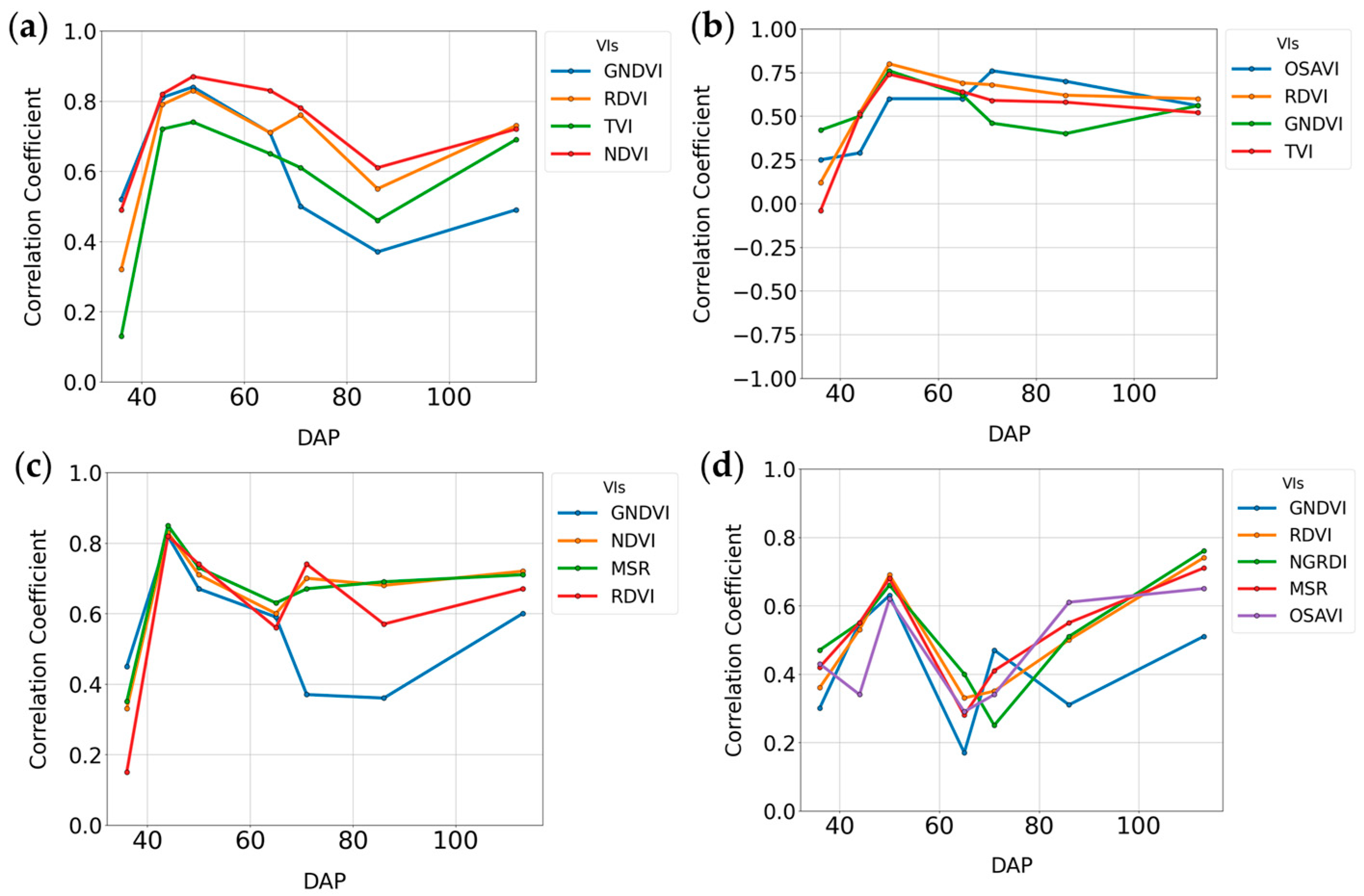
2.4.1. Spearman Correlation Rank
2.4.2. Feature Selection
2.4.3. Regression Models
2.5. Statistical Analysis
3. Results
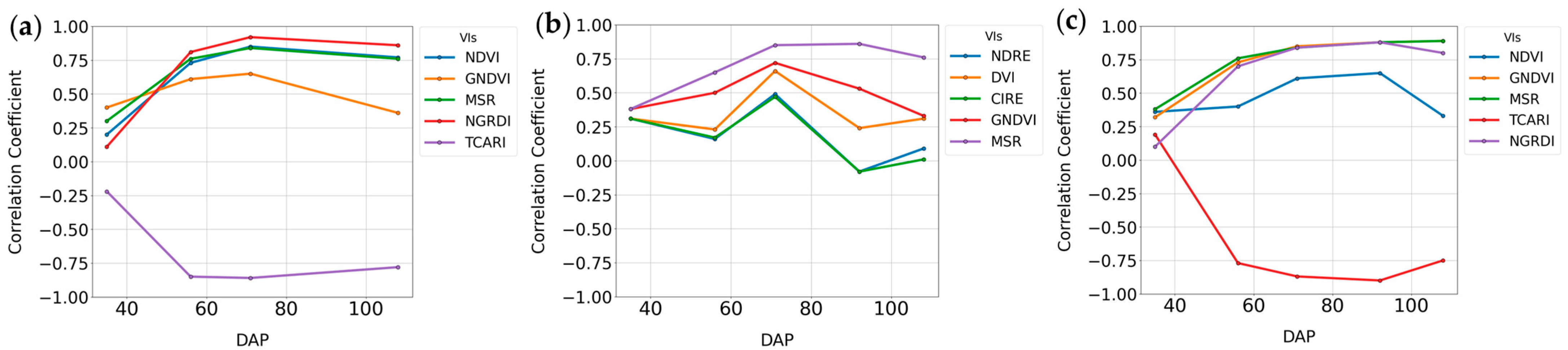
3.1. In-Season Growth Parameters
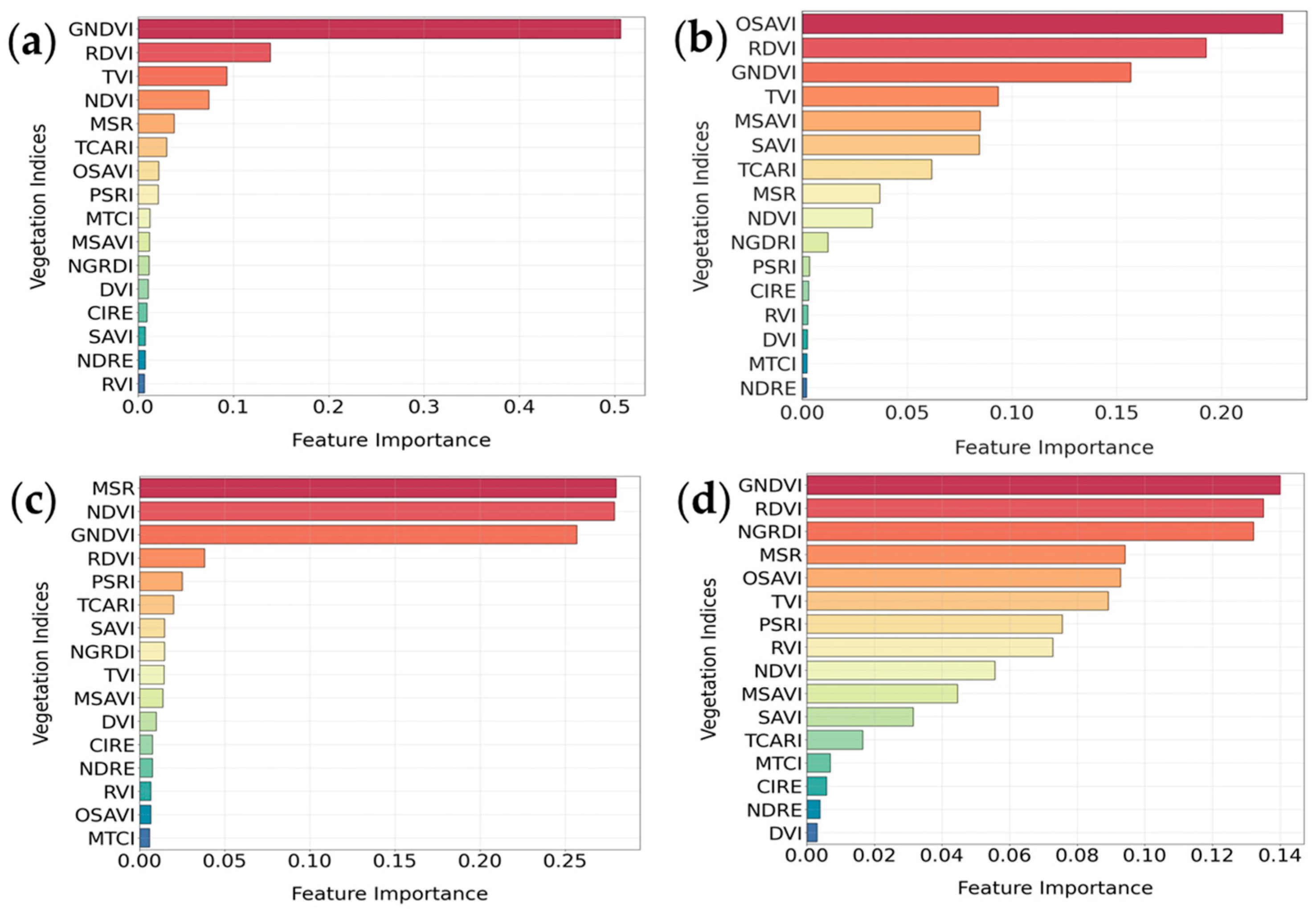
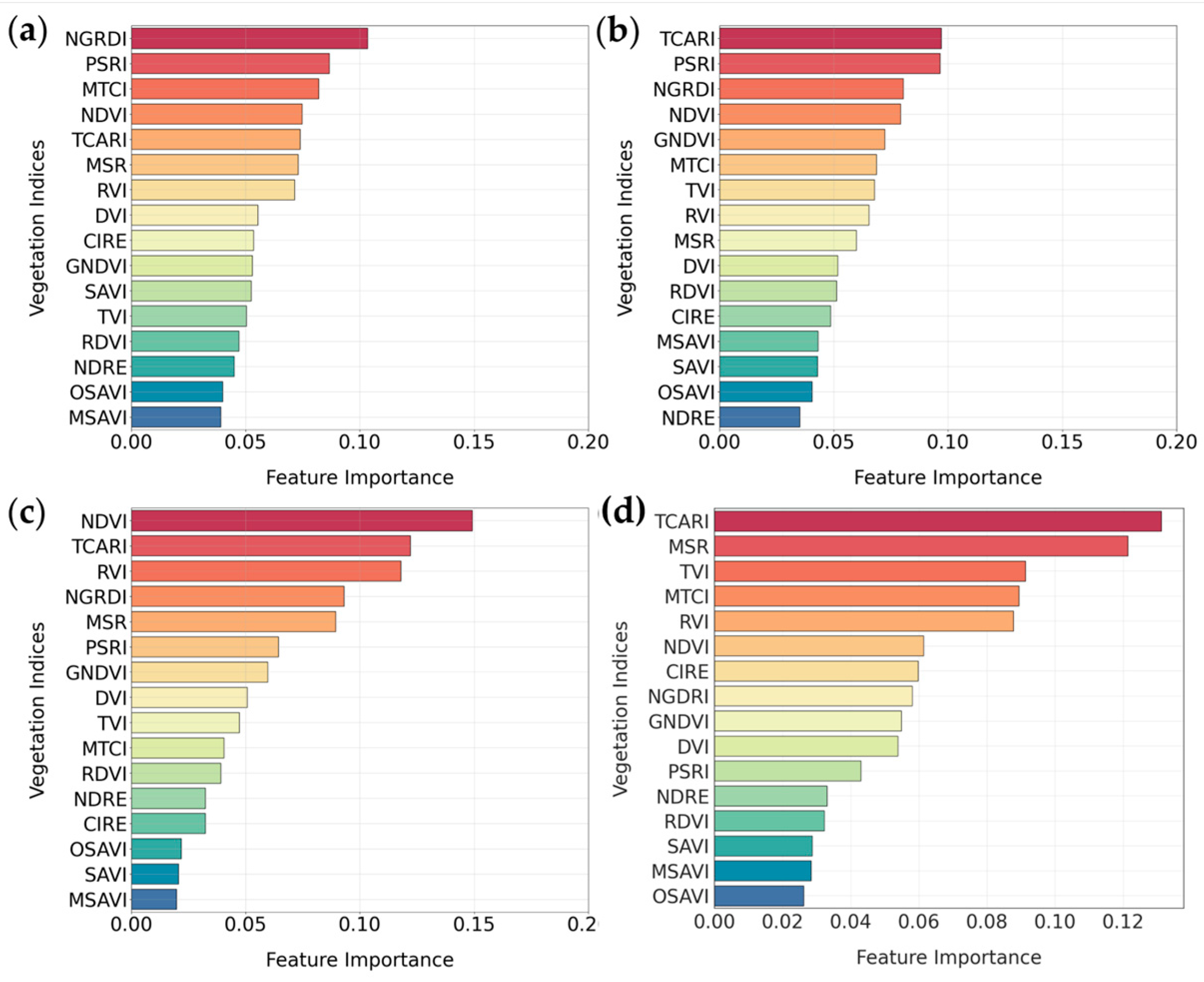
3.1.1. Random Forest Feature Selection Algorithm
3.1.2. Summary Statistics for Height, LAI, IPARf, and Mainstem Nodes
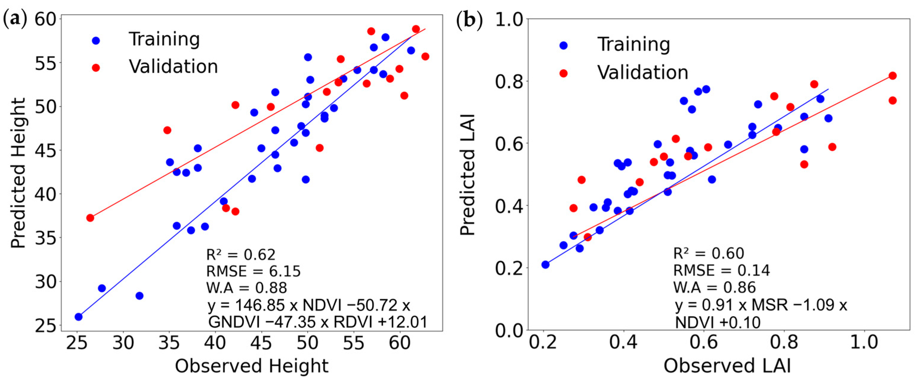
3.1.3. Regression Models for Height, LAI, IPARf, and Mainstem Nodes
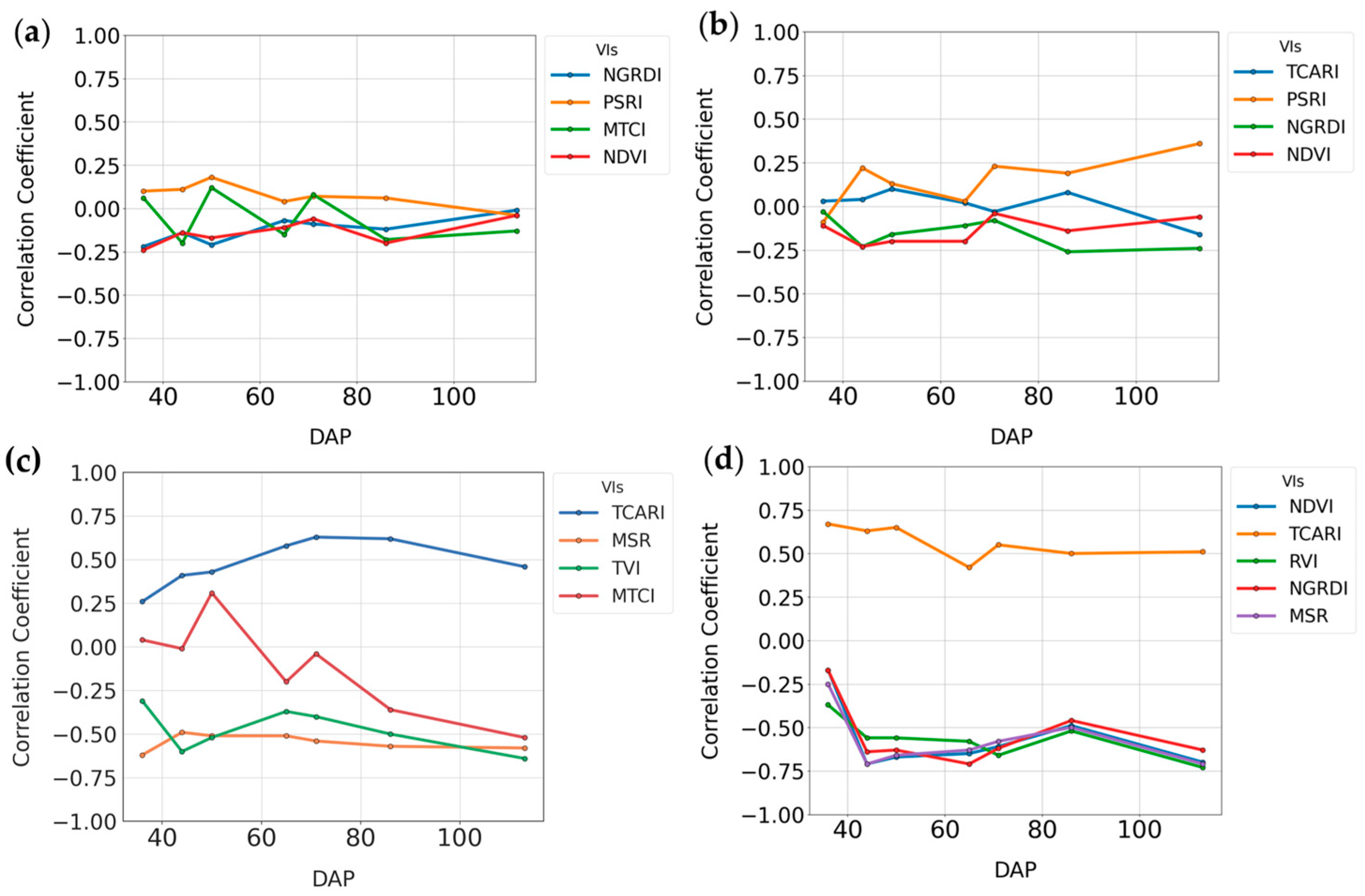
3.2. End-of-the-Season Parameters
3.2.1. Random Forest Feature Selection Algorithm
3.2.2. Summary Statistics for Lint Yield, Seed Yield, and Micronaire
3.2.3. Regression Models for Lint Yield, Seed Yield, and Micronaire
4. Discussion
4.1. In-Season Growth Parameters Estimation
4.2. End-of-the-Season Yield and Quality Parameters Estimation
4.3. Limitations
5. Conclusions
Author Contributions
Funding
Data Availability Statement
Acknowledgments
Conflicts of Interest
Appendix A
| 2018 | 2020 | ||||||
|---|---|---|---|---|---|---|---|
| Vegetation Indices | Height | Mainstem Nodes | LAI | IPARf | Height | LAI | IPARf |
| NDVI | 0.88 * | 0.82 * | 0.90 * | 0.95 * | 0.93 * | 0.88 * | 0.93 * |
| TVI | 0.87 * | 0.86 * | 0.85 * | 0.94 * | 0.84 * | 0.80 * | 0.81 * |
| NGRDI | 0.77 * | 0.69 * | 0.85 * | 0.92 * | 0.87 * | 0.87 * | 0.84 * |
| PSRI | −0.43 * | −0.38 * | −0.55 * | −0.62 * | −0.62 * | −0.60 * | −0.53 * |
| GNDVI | 0.93 * | 0.90 * | 0.88 * | 0.96 * | 0.88 * | 0.79 * | 0.89 * |
| NDRE | 0.67 * | 0.69 * | 0.73 * | 0.77 * | 0.73 * | 0.63 * | 0.75 * |
| CIRE | 0.67 * | 0.69 * | 0.73 * | 0.76 * | 0.74 * | 0.64 * | 0.76 * |
| DVI | 0.78 * | 0.80 * | 0.79 * | 0.84 * | 0.77 * | 0.71 * | 0.80 * |
| RDVI | 0.89 * | 0.87 * | 0.87 * | 0.96 * | 0.87 * | 0.84 * | 0.87 * |
| MSR | 0.88 * | 0.82 * | 0.91 * | 0.97 * | 0.92 * | 0.89 * | 0.93 * |
| MTCI | 0.50 * | 0.55 * | 0.58 * | 0.47 * | 0.67 * | 0.58 * | 0.70 * |
| SAVI | 0.87 * | 0.88 * | 0.83 * | 0.92 * | −0.25 * | −0.12 NS | −0.09 NS |
| RVI | 0.88 * | 0.84 * | 0.89 * | 0.96 * | 0.11 NS | 0.28 * | 0.34 * |
| MSAVI | 0.88 * | 0.89 * | 0.84 * | 0.93 * | −0.21 * | −0.09 NS | −0.06 NS |
| TCARI | −0.77 * | −0.77 * | −0.77 * | −0.94 * | −0.29 * | −0.43 * | −0.43 * |
| OSAVI | 0.89 * | 0.89 * | 0.85 * | 0.93 * | −0.18 NS | −0.07 NS | −0.03 NS |
| Variables | Year | Selected VIs |
|---|---|---|
| Height | 2018 | GNDVI, RDVI, TVI, NDVI |
| IPARf | OSAVI, RDVI, GNDVI, TVI | |
| LAI | MSR, NDVI, GNDVI, RDVI | |
| Nodes | GNDVI, RDVI, NGRDI, MSR, OSAVI | |
| Height | 2020 | NDVI, MSR, NGRDI, GNDVI, TCARI |
| IPARf | CIRE, DVI, MSR, GNDVI, NDRE | |
| LAI | NDVI, MSR, TCARI, GNDVI, NGRDI |
| 2018 | 2020 | |||||||
|---|---|---|---|---|---|---|---|---|
| Parameter | DAP | Range | Mean | SD | DAP | Range | Mean | SD |
| Height (cm) | 36 | 26.8–43.4 | 36.9 | 3.55 | 35 | 22.8–36.0 | 28.0 | 3.32 |
| 44 | 35.2–64.4 | 51.2 | 6.74 | 56 | 44.0–95.4 | 69.5 | 14.80 | |
| 50 | 25.1–62.7 | 47.3 | 9.51 | 71 | 56.2–128.2 | 90.6 | 20.13 | |
| 65 | 49.3–99.6 | 80.8 | 12.2 | 92 | 62.0–182.2 | 107.8 | 32.15 | |
| 71 | 67.1–125 | 101.2 | 12.3 | 108 | - | - | - | |
| 86 | 70.6–149.9 | 118.1 | 17.2 | |||||
| 113 | 78.2–175.3 | 129.4 | 24.5 | |||||
| LAI | 36 | 0.22–0.90 | 0.51 | 0.15 | 35 | 0.08–0.67 | 0.36 | 0.19 |
| 44 | 0.21–1.07 | 0.57 | 0.22 | 56 | 1.1–4.32 | 2.93 | 0.85 | |
| 50 | 0.43–2.6 | 1.03 | 0.40 | 71 | 1.77–7.03 | 4.49 | 1.33 | |
| 65 | 1.16–6.22 | 3.46 | 1.48 | 92 | 2.67–8.17 | 5.05 | 1.55 | |
| 71 | 2.00–7.62 | 5.38 | 1.44 | 108 | 2.17–6.74 | 4.24 | 1.42 | |
| 86 | 1.73–8.7 | 5.04 | 1.57 | |||||
| 113 | 1.87–5.67 | 4.09 | 0.78 | |||||
| IPARf | 36 | 0.08–0.25 | 0.18 | 0.03 | 35 | 0.01–0.23 | 0.12 | 0.06 |
| 44 | 0.13–0.50 | 0.27 | 0.10 | 56 | 0.37–0.94 | 0.79 | 0.13 | |
| 50 | 0.14–0.58 | 0.28 | 0.08 | 71 | 0.77–0.99 | 0.93 | 0.06 | |
| 65 | 0.37–0.91 | 0.76 | 0.13 | 92 | 0.87–1.00 | 0.96 | 0.04 | |
| 71 | 0.51–0.98 | 0.87 | 0.11 | 108 | 0.87–1.00 | 0.96 | 0.04 | |
| 86 | 0.61–0.99 | 0.93 | 0.08 | |||||
| 113 | 0.64–0.97 | 0.90 | 0.06 | |||||
| Nodes | 36 | 6.00–8.40 | 7.14 | 0.45 | ||||
| 44 | 8.40–11.00 | 9.79 | 0.60 | |||||
| 50 | 8.40–12.00 | 10.6 | 0.77 | |||||
| 65 | 11.6–16.20 | 14.1 | 0.94 | |||||
| 71 | 12.4–15.80 | 14.6 | 0.63 | |||||
| 86 | 14.60–19.80 | 17.4 | 1.14 | |||||
| 113 | 17.00–21.40 | 18.6 | 1.18 | |||||
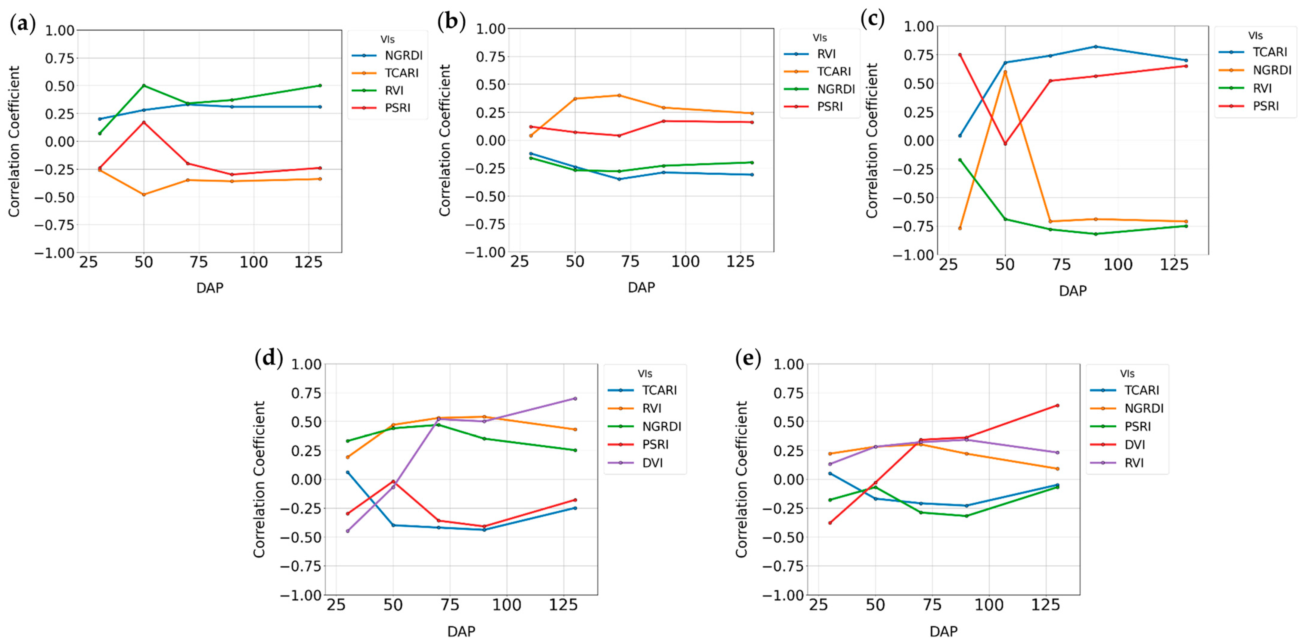
| 2018 | 2020 | ||||||||
|---|---|---|---|---|---|---|---|---|---|
| VIs | Lint Yield | Micronaire | Fiber Length | Fiber Strength | Lint Yield | Seed Yield | Micronaire | Fiber Length | Fiber Strength |
| NDVI | −0.29 * | −0.26 * | −0.06 NS | −0.07 NS | 0.15 NS | 0.25 * | −0.38 * | 0.20 * | −0.15 NS |
| TVI | −0.14 * | −0.17 * | −0.04 NS | −0.04 NS | 0.14 NS | 0.24 * | −0.37 * | 0.17 NS | −0.13 NS |
| NGRDI | −0.25 * | −0.20 * | −0.05 NS | −0.07 NS | 0.15 NS | 0.26 * | −0.47 * | 0.21 * | −0.18 * |
| PSRI | 0.11 * | 0.08 | 0.04 NS | 0.06 NS | −0.11 NS | −0.17 NS | 0.31 * | −0.12 | 0.10 NS |
| GNDVI | −0.19 * | −0.23 * | −0.03 NS | −0.04 NS | 0.13 NS | 0.20 * | −0.24 * | 0.15 NS | −0.11 NS |
| NDRE | −0.11 * | −0.07 | −0.03 NS | −0.04 NS | 0.13 NS | 0.15 NS | −0.07 NS | 0.08 NS | −0.01 NS |
| CIRE | −0.11 * | −0.07 | −0.03 NS | −0.04 NS | 0.12 NS | 0.14 NS | −0.06 NS | 0.08 NS | −0.01 NS |
| DVI | −0.13 * | −0.11 * | −0.04 NS | −0.03 NS | 0.14 NS | 0.18 * | −0.17 NS | 0.11 NS | −0.02 NS |
| RDVI | −0.18 * | −0.19 * | −0.04 NS | −0.05 NS | 0.15 NS | 0.24 * | −0.37 * | 0.19 * | −0.12 NS |
| MSR | −0.30 * | −0.27 * | −0.06 NS | −0.07 NS | 0.15 NS | 0.25 * | −0.39 * | 0.21 * | −0.15 NS |
| MTCI | −0.06 NS | −0.03 | −0.03 NS | −0.03 NS | 0.12 NS | 0.12 NS | −0.02 NS | 0.06 NS | 0.02 NS |
| SAVI | −0.15 * | −0.15 * | −0.04 NS | −0.02 NS | 0.15 NS | 0.24 * | −0.35 * | 0.20 * | −0.11 NS |
| RVI | −0.28 * | −0.24 * | −0.06 NS | −0.05 NS | 0.21 * | 0.34 * | −0.49 * | 0.27 * | −0.19 * |
| MSAVI | −0.16 * | −0.16 * | −0.05 NS | −0.03 NS | 0.15 NS | 0.25 * | −0.36 * | 0.20 * | −0.11 NS |
| TCARI | 0.21 * | 0.20 * | 0.01 NS | 0.00 NS | −0.14 NS | −0.29 * | 0.55 * | −0.30 * | 0.23 * |
| OSAVI | −0.19 * | −0.17 * | −0.05 NS | −0.03 NS | 0.17 * | 0.27 * | −0.38 * | 0.22 * | −0.11 NS |
| Variables | Year | Selected VIs |
|---|---|---|
| Fiber Length | 2018 | NGRDI, PSRI, MTCI, NDVI |
| Fiber Strength | TCARI, PSRI, NGRDI, NDVI | |
| Lint Yield | NDVI, TCARI, RVI, NGRDI, MSR | |
| Micronaire | NDVI, PSRI, DVI, NGRDI, MTCI | |
| Fiber Length | 2020 | NGRDI, TCARI, RVI, PSRI |
| Fiber Strength | RVI, TCARI, NGRDI, PSRI | |
| Lint Yield | TCARI, NGRDI, PSRI, DVI, RVI | |
| Seed Yield | TCARI, RVI, NGRDI, PSRI, DVI | |
| Micronaire | TCARI, NGRDI, RVI, PSRI |
| 2018 | 2020 | |||||
|---|---|---|---|---|---|---|
| Parameter | Range | Mean | SD | Range | Mean | SD |
| Fiber Length (cm) | 1.05–1.16 | 1.12 | 0.02 | 1.17–1.33 | 1.25 | 0.04 |
| Fiber Strength (g tex−1) | 25.1–34.5 | 30.8 | 2.03 | 28.7–32.5 | 30.3 | 0.90 |
| Micronaire | 3.2–5.1 | 4.09 | 0.45 | 3.5–4.9 | 4.31 | 0.35 |
| Lint Yield (kg.ha−1) | 314.29–2091.21 | 997.30 | 349.82 | 987.71–1742.95 | 1382.38 | 233.01 |
| Seed Yield (kg.ha−1) | - | - | - | 2562.22–4209.37 | 3492.37 | 502.48 |
References
- Khan, M.A.; Wahid, A.; Ahmad, M.; Tahir, M.T.; Ahmed, M.; Ahmad, S.; Hasanuzzaman, M. World cotton production and consumption: An overview. In Cotton Production and Uses: Agronomy, Crop Protection, and Postharvest Technologies; Springer: Singapore, 2020; pp. 321–340. [Google Scholar]
- MacDonald, S.; Lanclos, K.; Meyer, L.; Soley, G. Cotton Outlook. Agricultural Outlook Forum. 2024. Available online: https://www.usda.gov/about-usda/general-information/staff-offices/office-chief-economist/agricultural-outlook-forum/aof-commodity-outlooks (accessed on 6 May 2024).
- USDA-National Agricultural Statistics Service. Available online: https://www.nass.usda.gov/Quick_Stats/Ag_Overview/ (accessed on 5 May 2024).
- Hand, C.; Culpepper, S.; Vance, J.; Harris, G.; Kemerait, B.; Perry, C.; Hall, D.; Mallard, J.; Porter, W.; Roberts, P.; et al. 2023 Georgia Cotton Production Guide. Available online: https://extension.uga.edu/publications/detail.html?number=AP124-3&title=2023-georgia-cotton-production-guide (accessed on 6 May 2024).
- Chen, H.; Zhao, X.; Han, Y.; Xing, F.; Feng, L.; Wang, Z.; Wang, G.; Yang, B.; Lei, Y.; Xiong, S.; et al. Competition for Light Interception in Cotton Populations of Different Densities. Agronomy 2021, 11, 176. [Google Scholar] [CrossRef]
- Conaty, W.C.; Mahan, J.R.; Neilsen, J.E.; Tan, D.K.Y.; Yeates, S.Y.; Sutton, B.G. The relationship between cotton canopy temperature and yield, fibre quality and water-use efficiency. Field Crops Res. 2015, 183, 329–341. [Google Scholar] [CrossRef]
- Gao, M.; Snider, J.L.; Bai, H.; Hu, W.; Wang, R.; Meng, Y.; Wang, Y.; Chen, B.; Zhou, Z. Drought effects on cotton (Gossypium hirsutum L.) fibre quality and fibre sucrose metabolism during the flowering and boll-formation period. J. Agron. Crop Sci. 2020, 206, 309–321. [Google Scholar] [CrossRef]
- Chastain, D.R.; Snider, J.L.; Collins, G.D.; Perry, C.D.; Whitaker, J.; Byrd, S.A.; Oosterhuis, D.M.; Porter, W.M. Irrigation schedul-ing using predawn leaf water potential improves water productivity in drip-irrigated cotton. Crop Sci. 2016, 56, 3185–3195. [Google Scholar] [CrossRef]
- Monteith, J. LSolar radiation and productivity in tropical ecosystems. J. Appl. Ecol. 1972, 9, 747–766. [Google Scholar] [CrossRef]
- Shibles, R.M. Leaf area, solar radiation interception and dry matter production by soybeans. Crop Sci. 1965, 5, 575–577. [Google Scholar] [CrossRef]
- Ermanis, A.; Gobbo, S.; Snider, J.L.; Cohen, Y.; Liakos, V.; Lacerda, L.; Perry, C.D.; Bruce, M.A.; Virk, G.; Vellidis, G. Defining physiological contributions to yield loss in response to irrigation in cotton. J. Agron. Crop Sci. 2021, 207, 186–196. [Google Scholar] [CrossRef]
- Guo, S.; Han, Y.; Wang, G.; Wu, F.; Jia, Y.; Chen, J.; Li, X.; Du, W.; Li, Y.; Feng, L. Quantifying physiological contributions to yield loss in response to planting date in short-season cotton under a cotton-wheat double-cropping system. Eur. J. Agron. 2024, 154, 127089. [Google Scholar] [CrossRef]
- Feng, A.; Sudduth, K.; Vories, E.; Zhang, M.; Zhou, J. Cotton yield estimation based on plant height from UAV-based imagery data. Trans. ASABE 2018, 62, 393–403. [Google Scholar] [CrossRef]
- Lacerda, L.N.; Snider, J.; Cohen, Y.; Liakos, V.; Levi, M.R.; Vellidis, G. Correlation of UAV and satellite-derived vegetation indices with cotton physiological parameters and their use as a tool for scheduling variable rate irrigation in cotton. Precis. Agric. 2022, 23, 2089–2114. [Google Scholar] [CrossRef]
- Bradow, J.M.; Davidonis, G.H. Quantitation of fiber quality and the cotton production-processing interface: A physiologist’s perspective. J. Cotton Sci. 2000, 4, 34–64. [Google Scholar]
- Delhom, C.D.; Kelly, B.; Martin, V. Physical Properties of Cotton Fiber and Their Measurement. In Cotton Fiber: Physics, Chemistry and Biology; Fang, D., Ed.; Springer: Cham, Switzerland, 2018. [Google Scholar]
- Hinchliffe, D.J.; Meredith, W.R.; Delhom, C.D.; Thibodeaux, D.P.; Fang, D.D. Elevated growing degree days influence transition stage timing during cotton fiber development resulting in increased fiber-bundle strength. Crop Sci. 2011, 51, 1683–1692. [Google Scholar] [CrossRef]
- Fang, D.D. General Description of Cotton. In Cotton Fiber: Physics, Chemistry and Biology; Fang, D., Ed.; Springer: Cham, Switzerland, 2018. [Google Scholar]
- Kothari, N.; Hague, S.; Hinze, L.; Dever, J. Boll sampling protocols and their impact on measurements of cotton fiber quality. Ind. Crops Prod. 2017, 109, 248–254. [Google Scholar] [CrossRef]
- Siddiqui, M.Q.; Wang, H.; Memon, H. Cotton Fiber Testing. In Cotton Science and Processing Technology. Textile Science and Clothing Technology; Wang, H., Memon, H., Eds.; Springer: Singapore, 2020. [Google Scholar]
- Xu, W.; Yang, W.; Chen, P.; Zhan, Y.; Zhang, L.; Lan, Y. Cotton Fiber Quality Estimation Based on Machine Learning Using Time Series UAV Remote Sensing Data. Remote Sens. 2023, 15, 586. [Google Scholar] [CrossRef]
- Yeom, J.; Jung, J.; Chang, A.; Maeda, M.; Landivar, J. Automated Open Cotton Boll Detection for Yield Estimation Using Unmanned Aircraft Vehicle (UAV) Data. Remote Sens. 2018, 10, 1895. [Google Scholar] [CrossRef]
- Wu, J.; Wen, S.; Lan, Y.; Zhang, J.; Ge, Y. Estimation of cotton canopy parameters based on unmanned aerial vehicle (UAV) oblique photography. Plant Methods 2022, 18, 129. [Google Scholar] [CrossRef]
- Xu, W.; Yang, W.; Chen, S.; Wu, C.; Chen, P.; Lan, Y. Establihsing a model to predict the single boll weight of cotton in northern Xinjiang by using high resolution UAV remote sensing data. Comput. Electron. Agric. 2020, 179, 105762. [Google Scholar] [CrossRef]
- Feng, A.; Zhou, J.; Vories, E.D.; Sudduth, K.A.; Zhang, M. Yield estimation in cotton using UAV-based multi-sensor imagery. Biosyst. Eng. 2020, 193, 101–114. [Google Scholar] [CrossRef]
- Pokhrel, A.; Virk, S.; Snider, J.L.; Vellidis, G.; Hand, L.C.; Sintim, H.Y.; Parkash, V.; Chalise, D.P.; Lee, J.M.; Byers, C. Estimating yield-contributing physiological parameters of cotton using UAV-based imagery. Front. Plant Sci. 2023, 14, 1248152. [Google Scholar] [CrossRef]
- Chalise, D.P.; Snider, J.L.; Hand, L.C.; Roberts, P.; Vellidis, G.; Ermanis, A.; Collins, G.D.; Lacerda, L.N.; Cohen, Y.; Pokhrel, A.; et al. Cultivar, irrigation management, and mepiquat chloride strategy: Effects on cotton growth, maturity, yield, and fiber quality. Field Crops Res. 2022, 286, 108633. [Google Scholar] [CrossRef]
- Vellidis, G.; Liakos, V.; Andreis, J.H.; Perry, C.D.; Porter, W.M.; Barnes, E.M.; Morgan, K.T.; Fraisse, C.; Migliaccio, K.W. Development and assessment of a smartphone application for irrigation scheduling in cotton. Comput. Electron. Agric. 2016, 127, 249–259. [Google Scholar] [CrossRef]
- Lacerda, L.N.; Snider, J.L.; Cohen, Y.; Liakos, V.; Gobbo, S.; Vellidis, G. Using UAV-based thermal imagery to detect crop water status variability in cotton. Smart Agric. Technol. 2022, 2, 100029. [Google Scholar] [CrossRef]
- Ritchie, G.L.; Bednarz, C.W.; Jost, P.H.; Brown, S.M. Cotton Growth and Development. 2007 Jun 1; Cooperative Extension Work of University of Georgia Bulletin 1252. Available online: https://hdl.handle.net/10724/12192 (accessed on 6 May 2024).
- Matias, F.I.; Caraza-Harter, M.V.; Endelman, J.B. FIELDimageR: An R package to analyze orthomosaic images from agricultural field trials. Plant Phenome J. 2020, 3, e20005. [Google Scholar] [CrossRef]
- Jones, H.G.; Vaughan, R.A. Remote Sensing of Vegetation: Principles, Techniques, and Applications; Oxford University Press: New York, NY, USA, 2010; p. 353. [Google Scholar]
- Pawar, P.S.; Matias, F.I. FIELDimageR.Extra: Advancing user experience and computational efficiency for analysis of orthomosaic from agricultural field trials. Plant Phenome J. 2023, 6, e20083. [Google Scholar] [CrossRef]
- Barboza, T.O.C.; Ardigueri, M.; Souza, G.F.C.; Ferraz, M.A.J.; Gaudencio, J.R.F.; Santos, A.F.D. Performance of Vegetation Indices to Estimate Green Biomass Accumulation in Common Bean. AgriEngineering 2023, 5, 840–854. [Google Scholar] [CrossRef]
- Hott, M.C.; Andrade, R.G.; de Magalhaes, W.C.P., Jr.; Benites, F.R.G. Uso de veículo aéreo não tripulado (VANT) para estimativa de vigor e de correlações agronômicas em genótipos de capim cynodon. In Engenharia Sanitária e Ambiental; Atena Editora: Ponta Grossa, Brazil, 2018; Chapter 22; pp. 235–244. [Google Scholar]
- Sims, D.A.; Gamon, J.A. Relationships between leaf pigment content and spectral reflectance across a wide range of species, leaf structures and developmental stages. Remote Sens. Environ. 2002, 81, 337–354. [Google Scholar] [CrossRef]
- Kogan, F.; Gitelson, A.; Zakarin, E.; Spivak, L.; Lebed, L. AVHRR-based spectral vegetation index for quantitative assessment of vegetation state and productivity: Calibration and validation. Photogramm. Eng. Remote Sens. 2003, 69, 899–906. [Google Scholar] [CrossRef]
- Jordan, C.F. Derivation of Leaf-Area Index from Quality of Light on the Forest Floor. Ecology 1969, 50, 663–666. [Google Scholar] [CrossRef]
- Gitelson, A.; Merzlyak, M.N. Spectral Reflectance Changes Associated with Autumn Senescence of Aesculus hippocastanum L. and Acer platanoides L. Leaves. Spectral Features and Relation to Chlorophyll Estimation. J. Plant Physiol. 1994, 143, 286–292. [Google Scholar] [CrossRef]
- Gitelson, A.A.; Kaufman, Y.J.; Merzlyak, M.N. Use of a green channel in remote sensing of global vegetation from EOS-MODIS. Remote Sens. Environ. 1996, 58, 289–298. [Google Scholar] [CrossRef]
- Roujean, J.L.; Boreon, F.M. Estimating PAR absorbed by vegetation from bidirectional reflectance measurements. Remote Sens. Environ. 1995, 51, 375–384. [Google Scholar] [CrossRef]
- Tucker, C.J. Red and photographic infrared linear combinations for monitoring vegetation. Remote Sens. Environ. 1979, 8, 127–150. [Google Scholar] [CrossRef]
- Haboudane, D.; Miller, J.R.; Tremblay, N.; Zarco-Tejada, P.J.; Dextraze, L. Integrated narrow-band vegetation indices for prediction of crop chlorophyll content for application to precision agriculture. Remote Sens. Environ. 2002, 81, 416–426. [Google Scholar] [CrossRef]
- Rouse, J.W. Monitoring the Vernal Advancement and Retrogradation of Natural Vegetation (Green Wave Effect) of Natural Vegetation; Texas A&M University: College Station, TX, USA; National Aeronautics and Space Administration: Washington, DC, USA, 1974; p. 371.
- Merzlyak, M.N.; Gitelson, A.A.; Chivkunova, O.B.; Rakitin, V.Y.U. Non-destructive optical detection of pigment changes during leaf senescence and fruit ripening. Physiol. Plant. 1999, 106, 135–141. [Google Scholar] [CrossRef]
- Broge, N.H.; Leblanc, E. Comparing prediction power and stability of broadband and hyperspectral vegetation indices for estimation of green leaf area index and canopy chlorophyll density. Remote Sens. Environ. 2001, 76, 156–172. [Google Scholar] [CrossRef]
- Chen, J. Evaluation of vegetation indices and modified simple ratio for boreal applications. Can. J. Remote Sens. 1996, 22, 229–242. [Google Scholar] [CrossRef]
- Dash, J.; Curran, P. The MERIS terrestrial chlorophyll index. Int. J. Remote Sens. 2004, 25, 5403–5413. [Google Scholar] [CrossRef]
- Qi, J.; Chehbouni, A.; Huete, A.R.; Kerr, Y.H.; Sorooshian, S. A modified soil adjusted vegetation index. Remote Sens. Environ. 1994, 48, 119–126. [Google Scholar] [CrossRef]
- Huete, A.R. A soil-adjusted vegetation index (SAVI). Remote Sens. Environ. 1998, 25, 295–309. [Google Scholar] [CrossRef]
- Pearson, R.L.; Miller, L.D. Remote mapping of standing crop biomass for estimation of the productivity of the short-grass Prairie, Pawnee National Grassland, Colorado. In Proceedings of the 8th International Symposium on Remote Sensing of Environment, Ann Arbor, MI, USA, 2–6 October 1972; pp. 1357–1381. [Google Scholar]
- Rondeaux, G.; Steven, M.; Baret, F. Optimization of soil-adjusted vegetation indices. Remote Sens. Environ. 1996, 55, 95–107. [Google Scholar] [CrossRef]
- Spearman, C. The Proof and Measurement of Association Between Two Things. In Studies in Individual Differences: The Search for Intelligence; Jenkins, J.J., Paterson, D.G., Eds.; Appleton-Century-Crofts: New York, NY, USA, 1961; pp. 45–58. [Google Scholar]
- de Winter, J.C.F.; Gosling, S.D.; Potter, J. Comparing the Pearson and Spearman correlation coefficients across distributions and sample sizes: A tutorial using simulations and empirical data. Psychol. Methods 2016, 21, 273–290. [Google Scholar] [CrossRef]
- Breiman, L. Random Forests. Mach. Learn. 2001, 45, 5–32. [Google Scholar] [CrossRef]
- Díaz-Uriarte, R.; Andrés, S.A. Gene selection and classification of microarray data using random forest. BMC Bioinform. 2006, 7, 3. [Google Scholar] [CrossRef]
- Degenhardt, F.; Seifert, S.; Szymczak, S. Evaluation of variable selection methods for random forests and omics data sets. Brief. Bioinform. 2019, 20, 492–503. [Google Scholar] [CrossRef] [PubMed]
- Pedregosa, F.; Varoquaux, G.; Gramfort, A.; Michel, V.; Thirion, B.; Grisel, O.; Blondel, M.; Prettenhofer, P.; Weiss, R.; Dubourg, V.; et al. Scikit-learn: Machine learning in python. J. Mach. Learn. Res. 2011, 12, 2825–2830. [Google Scholar]
- Waskom, M.L. seaborn: Statistical data visualization. J. Open Source Softw. 2021, 6, 3021. [Google Scholar] [CrossRef]
- Hunter, J.D. Matplotlib: A 2D Graphics Environment. Comput. Sci. Eng. 2007, 9, 90–95. [Google Scholar] [CrossRef]
- Willmott, C.J.; Ackleson, S.G.; Davis, R.E.; Feddema, J.J.; Klink, K.M.; Legates, D.R.; O’Donnell, J.; Rowe, C.M. Statistics for the evaluation and comparison of models. J. Geophys. Res. 1985, 90, 8995–9005. [Google Scholar] [CrossRef]
- Snider, J.; Harris, G.; Roberts, P.; Meeks, C.; Chastain, D.; Bange, M.; Virk, G. Cotton physiological and agronomic response to nitrogen application rate. Field Crops Res. 2021, 270, 108194. [Google Scholar] [CrossRef]
- Pádua, L.; Antão-Geraldes, A.M.; Sousa, J.J.; Rodrigues, M.Â.; Oliveira, V.; Santos, D.; Miguens, M.F.P.; Castro, J.P. Water Hyacinth (Eichhornia crassipes) Detection Using Coarse and High-Resolution Multispectral Data. Drones 2022, 6, 47. [Google Scholar] [CrossRef]
- Ma, Y.; Zhang, Q.; Yi, Q.; Ma, L.; Zhang, L.; Huang, C.; Zhang, Z.; Lv, X. Estimation of cotton leaf area index (LAI) based on spectral transformation and vegetation index. Remote Sens. 2022, 14, 136. [Google Scholar] [CrossRef]
- Qi, Y.; Chen, X.; Chen, Z.; Zhang, X.; Shen, C.; Chen, Y.; Peng, Y.; Chen, B.; Wang, Q.; Liu, T.; et al. Estimation Model for Cotton Canopy Structure Parameters Based on Spectral Vegetation Index. Life 2025, 15, 62. [Google Scholar] [CrossRef]
- Bronson, K.F.; Conley, M.M.; French, A.N.; Hunsaker, D.J.; Thorp, K.R.; Barness, E.M. Which active optical sensor vegetation index is best for nitrogen assessment in irrigated cotton? Agron. J. 2020, 112, 2205–2218. [Google Scholar] [CrossRef]
- Pazhanivelan, S.; Kumaraperumal, R.; Shanmugapriya, P.; Sudarmanian, N.S.; Sivamurugan, A.P.; Satheesh, S. Quantification of biophysical parameters and economic yield in cotton and rice using drone technology. Agriculture 2023, 13, 1668. [Google Scholar] [CrossRef]
- Sims, D.A.; Gamon, J.A. Estimation of vegetation water content and photosynthetic tissue area from spectral reflectance: A comparison of indices based on liquid water and chlorophyll absorption features. Remote Sens. Environ. 2003, 84, 526–537. [Google Scholar] [CrossRef]
- Wanjura, D.F.; Hatfield, J.L. Sensitivity of spectral vegetation indices to crop biomass. ASABE 1986, 30, 810–816. [Google Scholar]
- Raper, T.B.; Varco, J.J. Canopy-scale wavelength and vegetative index sensitivities to cotton growth parameters and nitrogen status. Precis. Agric. 2015, 16, 62–76. [Google Scholar] [CrossRef]
- Reddy, K.R.; Zhao, D.; Kakani, V.G.; Read, J.J.; Sailaja, K. Estimating cotton growth and developmental parameters through remote sensing. In Ecosystems’ Dynamics, Agricultural Remote Sensing and Modeling, and Site-Specific Agriculture; SPIE: Bellingham, WA, USA, 2003; Volume 5153. [Google Scholar]
- Pettigrew, W.T. Low light conditions compromise the quality of fiber produced. In Proceedings of the 1996 Beltwide Cotton Conferences, Nashville, TN, USA, 9–12 January 1996; National Cotton Council of America: Memphis, TN, USA, 1996. [Google Scholar]
- Percy, R.G.; Cantrell, R.G.; Zhang, J. Genetic variation for agronomic and fiber properties in an introgressed recombinant inbred population of cotton. Crop Sci. 2006, 46, 1311–1317. [Google Scholar] [CrossRef]
- Yeates, S.J.; Constable, G.A.; McCumstie, T. Irrigated cotton in the tropical dry season. I: Yield, its components and crop development. Field Crops Res. 2010, 116, 278–289. [Google Scholar] [CrossRef]
- Jia, Y.; Yang, B.; Han, Y.; Wang, G.; Su, T.; Li, X.; Lei, Y.; Zhi, X.; Xiong, S.; Xin, M.; et al. Enhanced Cotton Yield and Fiber Quality by Optimizing Irrigation Amount and Frequency in Arid Areas of Northwest China. Agronomy 2024, 14, 266. [Google Scholar] [CrossRef]
- Bai, Z.; Bai, W.; Xie, C.; Yu, J.; Dai, Y.; Pei, S.; Zhang, F.; Li, Y.; Fan, J.; Yin, F. Irrigation depth and nitrogen rate effects on seed cotton yield, fiber quality and water-nitrogen utilization efficiency in southern Xinjiang, China. Agric. Water Manag. 2023, 290, 108583. [Google Scholar] [CrossRef]
- Bange, M.P.; Long, R.L.; Caton, S.J.; Finger, N. Prediction of upland cotton micronaire accounting for the effects of environment and crop demand from fruit growth. Crop Sci. 2022, 62, 397–409. [Google Scholar] [CrossRef]
- Haghverdi, A.; Washington-Allen, R.A.; Leib, B.G. Prediction of cotton lint yield from phenology of crop indices using artificial neural networks. Comput. Electron. Agric. 2018, 152, 186–197. [Google Scholar] [CrossRef]
- Shi, G.; Du, X.; Du, M.; Li, Q.; Tian, X.; Ren, Y.; Zhang, Y.; Wang, H. Cotton Yield Estimation Using the Remotely Sensed Cotton Boll Index from UAV Images. Drones 2022, 6, 254. [Google Scholar] [CrossRef]


| Growth Stage | Days After Planting (DAP) |
|---|---|
| Emergence | 5 |
| First Square | 38 |
| First Flower | 59 |
| Open Boll | 116 |
| Harvest | 140 |
| Growth Parameter | Model Input Variables | Model | R2 | RMSE | Willmott Agreement | R2 | RMSE | Willmott Agreement |
|---|---|---|---|---|---|---|---|---|
| 2018 | ||||||||
| Training | Validation | |||||||
| Height (50 DAP) | NDVI | Linear | 0.80 | 3.90 | 0.94 | 0.62 | 6.17 | 0.88 |
| NDVI, GNDVI, RDVI * | Multiple * | 0.81 | 3.79 | 0.94 | 0.62 | 6.15 | 0.88 | |
| Polynomial | 0.83 | 3.90 | 0.95 | 0.60 | 5.99 | 0.81 | ||
| IPARf (50 DAP) | RDVI * | Linear * | 0.65 | 0.04 | 0.89 | 0.30 | 0.08 | 0.60 |
| RDVI, GNDVI, TVI, OSAVI | Multiple | 0.78 | 0.03 | 0.93 | 0.21 | 0.08 | 0.63 | |
| Polynomial | 0.62 | 0.05 | 0.86 | 0.28 | 0.04 | 0.71 | ||
| LAI (44 DAP) | MSR | Linear | 0.65 | 0.10 | 0.89 | 0.52 | 0.17 | 0.83 |
| MSR, NDVI * | Multiple * | 0.65 | 0.11 | 0.88 | 0.60 | 0.14 | 0.86 | |
| Polynomial | 0.67 | 0.11 | 0.89 | 0.61 | 0.18 | 0.77 | ||
| Mainstem Nodes (50 DAP) | RDVI | Linear | 0.38 | 0.49 | 0.74 | 0.19 | 0.45 | 0.69 |
| RDVI, MSR, NGRDI, GNDVI, OSAVI * | Multiple * | 0.54 | 0.47 | 0.82 | 0.44 | 0.71 | 0.67 | |
| Polynomial | 0.67 | 0.4 | 0.89 | 0.19 | 0.84 | 0.41 | ||
| 2020 | ||||||||
| Height (71 DAP) | NGRDI | Linear | 0.83 | 8.12 | 0.77 | - | - | - |
| NGRDI, NDVI, MSR, GNDVI, TCARI * | Multiple | 0.88 | 6.7 | 0.96 | - | - | - | |
| Polynomial * | 0.96 | 3.9 | 0.98 | - | - | - | ||
| LAI (71 DAP) | MSR | Linear | 0.78 | 0.61 | 0.77 | - | - | - |
| MSR, TCARI, NDVI, NGRDI, GNDVI * | Multiple | 0.81 | 0.57 | 0.77 | - | - | - | |
| Polynomial * | 0.87 | 0.47 | 0.83 | - | - | - | ||
| IPARf (71 DAP) | MSR | Linear | 0.63 | 0.04 | 0.59 | - | - | - |
| MSR, GNDVI, DVI, NDRE, CIRE * | Multiple | 0.77 | 0.83 | 0.77 | - | - | - | |
| Polynomial * | 0.91 | 0.02 | 0.86 | - | - | - | ||
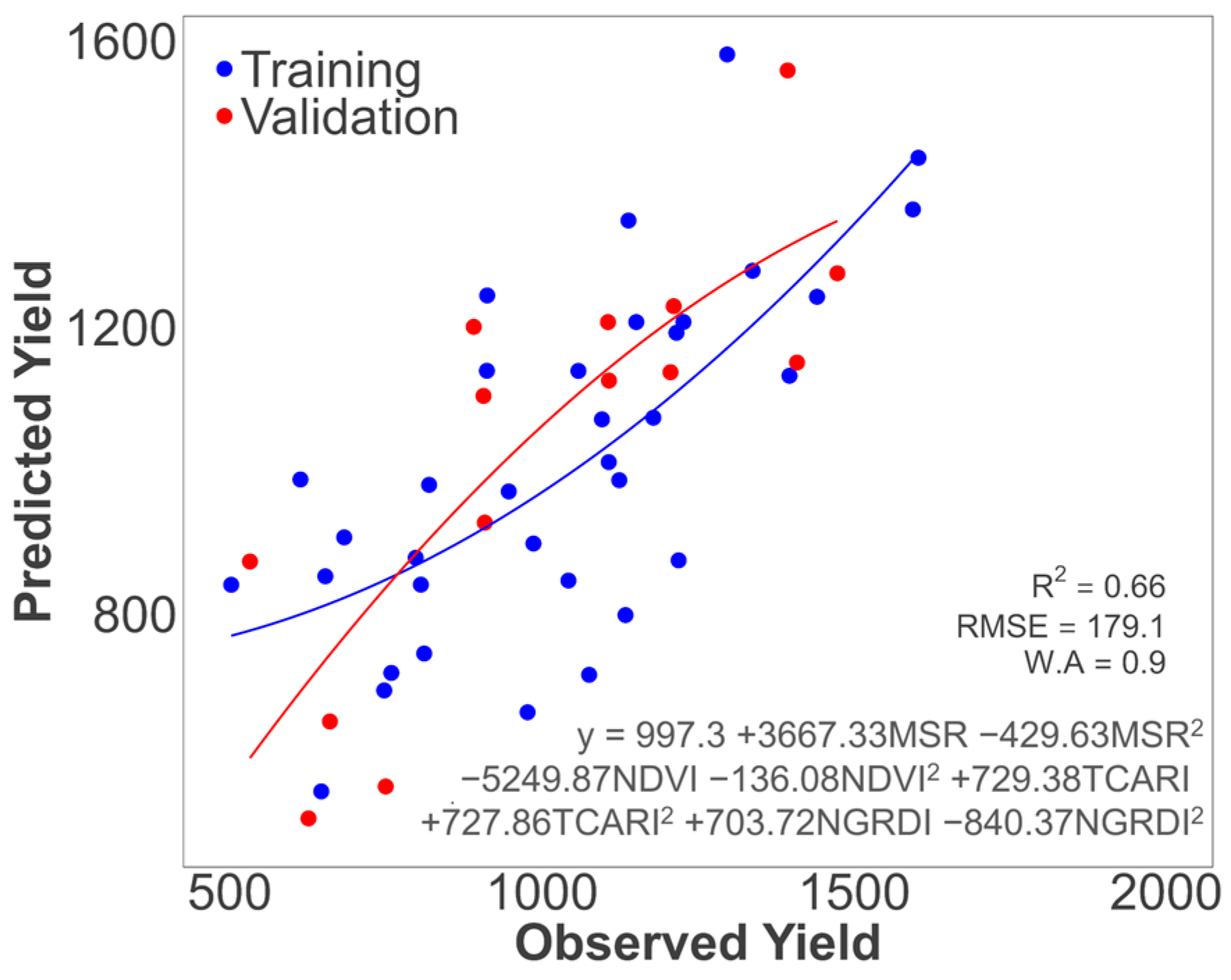
| Parameter | Model Input Variables | Model | R2 | RMSE | Willmott Agreement | R2 | RMSE | Willmott Agreement |
|---|---|---|---|---|---|---|---|---|
| 2018 | ||||||||
| Training | Validation | |||||||
| Lint Yield (44 DAP) | MSR | Linear | 0.41 | 271.23 | 0.76 | 0.22 | 244.29 | 0.73 |
| MSR, NDVI, TCARI, NGRDI, RVI | Multiple | 0.50 | 250.16 | 0.81 | 0.19 | 248.18 | 0.76 | |
| Polynomial | 0.58 | 236.48 | 0.84 | 0.67 | 174.68 | 0.90 | ||
| MSR, NDVI, TCARI, NGRDI * | Multiple | 0.49 | 250.84 | 0.81 | 0.17 | 251.70 | 0.76 | |
| Polynomial * | 0.58 | 235.77 | 0.84 | 0.66 | 179.10 | 0.89 | ||
| Micronaire (86 DAP) | TCARI | Linear | 0.38 | 0.35 | 0.7 | 0.2 | 0.37 | 0.68 |
| TCARI, MSR | Multiple | 0.45 | 0.32 | 0.7 | 0.33 | 0.41 | 0.73 | |
| Polynomial * | 0.50 | 0.31 | 0.81 | 0.30 | 0.41 | 0.66 | ||
| 2020 | ||||||||
| Lint Yield (108 DAP) | DVI | Linear | 0.43 | 171.24 | 0.54 | - | - | - |
| DVI, RVI, NGRDI, PSRI, TCARI * | Multiple | 0.51 | 159.91 | 0.57 | - | - | - | |
| Polynomial * | 0.76 | 111.32 | 0.92 | - | - | - | ||
| Seed Yield (108 DAP) | DVI | Linear | 0.55 | 327.33 | 0.60 | - | - | - |
| DVI, RVI, NGRDI, TCARI, PSRI * | Multiple | 0.63 | 295.87 | 0.67 | - | - | - | |
| Polynomial * | 0.73 | 253.6 | 0.91 | - | - | - | ||
| Micronaire (71 DAP) | RVI | Linear | 0.56 | 0.22 | 0.65 | - | - | - |
| RVI, NGRDI, TCARI, PSRI * | Multiple | 0.60 | 0.21 | 0.66 | - | - | - | |
| Polynomial * | 0.68 | 0.19 | 0.89 | - | - | - | ||
Disclaimer/Publisher’s Note: The statements, opinions and data contained in all publications are solely those of the individual author(s) and contributor(s) and not of MDPI and/or the editor(s). MDPI and/or the editor(s) disclaim responsibility for any injury to people or property resulting from any ideas, methods, instructions or products referred to in the content. |
© 2025 by the authors. Licensee MDPI, Basel, Switzerland. This article is an open access article distributed under the terms and conditions of the Creative Commons Attribution (CC BY) license (https://creativecommons.org/licenses/by/4.0/).
Share and Cite
Lacerda, L.N.; Ardigueri, M.; C. Barboza, T.O.; Snider, J.; Chalise, D.P.; Gobbo, S.; Vellidis, G. Using High-Resolution Multispectral Data to Evaluate In-Season Cotton Growth Parameters and End-of-the-Season Cotton Fiber Yield and Quality. Agronomy 2025, 15, 692. https://doi.org/10.3390/agronomy15030692
Lacerda LN, Ardigueri M, C. Barboza TO, Snider J, Chalise DP, Gobbo S, Vellidis G. Using High-Resolution Multispectral Data to Evaluate In-Season Cotton Growth Parameters and End-of-the-Season Cotton Fiber Yield and Quality. Agronomy. 2025; 15(3):692. https://doi.org/10.3390/agronomy15030692
Chicago/Turabian StyleLacerda, Lorena N., Matheus Ardigueri, Thiago O. C. Barboza, John Snider, Devendra P. Chalise, Stefano Gobbo, and George Vellidis. 2025. "Using High-Resolution Multispectral Data to Evaluate In-Season Cotton Growth Parameters and End-of-the-Season Cotton Fiber Yield and Quality" Agronomy 15, no. 3: 692. https://doi.org/10.3390/agronomy15030692
APA StyleLacerda, L. N., Ardigueri, M., C. Barboza, T. O., Snider, J., Chalise, D. P., Gobbo, S., & Vellidis, G. (2025). Using High-Resolution Multispectral Data to Evaluate In-Season Cotton Growth Parameters and End-of-the-Season Cotton Fiber Yield and Quality. Agronomy, 15(3), 692. https://doi.org/10.3390/agronomy15030692