Abstract
Autonomous navigation is key to improving efficiency and addressing labor shortages in the fruit industry. Semi-structured orchards, with straight tree rows, dense weeds, thick canopies, and varying light conditions, pose challenges for tree identification and navigation line extraction. Traditional 3D lidars suffer from a narrow vertical FoV, sparse point clouds, and high costs. Furthermore, most lidar-based tree-row-detection algorithms struggle to extract high-quality navigation lines in scenarios with thin trunks and dense foliage occlusion. To address these challenges, we developed a 3D perception system using a servo motor to control the rolling motion of a 2D lidar, constructing 3D point clouds with a wide vertical FoV and high resolution. In addition, a method for trunk feature point extraction and tree row line detection for autonomous navigation has been proposed, based on trunk geometric features and RANSAC. Outdoor tests demonstrate the system’s effectiveness. At speeds of 0.2 m/s and 0.5 m/s, the average distance errors are 0.023 m and 0.016 m, respectively, while the average angular errors are 0.272° and 0.146°. This low-cost solution overcomes traditional lidar-based navigation method limitations, making it promising for autonomous navigation in semi-structured orchards.
1. Introduction
The fruit industry is significant to the rural economic development and food security in China, yielding 327.4428 million tons in 2023 (https://www.chinairn.com/hyzx/20240912/110302208.shtml, accessed on 21 September 2024). However, increasing labor costs and the aging population in China have caused a severe labor shortage in orchards [1]. Fortunately, artificial intelligence (AI) and embodied AI make agricultural robots a promising solution to harvesting, pruning, and spraying in orchards, which can not only solve the problem of labor shortage but also increase working efficiency [2]. In particular, autonomous navigation as a crucial technique could guide robots to move automatically and safely within the work area, making it fundamental to autonomous operation in orchards.
Nowadays, modern orchards have become the mainstream mode of fruit cultivation and production, where trees are planted in straight and parallel rows, forming a semi-structured workspace [3]. Considering this semi-structured tree cultivation, autonomous navigation in orchards can be simply described as the robot traveling from the beginning to the end of the tree row and performing a U-turn to the next tree row, repeating this process until it covers the entire workspace [4]. This working mode requires sensors to perceive and extract the tree row information for accurate positioning and stable guidance in orchards with thick canopies, dense weeds, and varying illuminations. The Global Navigation Satellite System (GNSS) combined with Real-Time Kinematic (RTK) technology achieves good performance in autonomous navigation in farms and fields [5]. Nevertheless, the interference of fruit tree branches and dense canopies in orchards can lead to unstable or even lost satellite signals, thereby affecting the reliability and safety of autonomous navigation [6]. In contrast, lidar is not affected by signal interference because it does not require external signals to obtain positioning information [7]. Furthermore, lidar is insensitive to changing illumination, which most optical sensors suffer from [8,9,10,11].
Additionally, lidar is typically classified into 2D and 3D types, based on its data measurement dimension. The 2D lidar has been proven effective in autonomous navigation in orchards by scanning trunks to determine the lidar’s relative position within the tree row [12,13,14,15,16]. However, 2D lidar makes it difficult to extract the tree row information due to the occlusion of tree trunks by weeds and foliage in orchards [17]. In comparison, 3D lidar can additionally obtain objects’ height to capture precise 3D contour information of the environment, which is more conducive to detecting environmental obstacles and achieving more reliable navigation [18,19,20].
Unfortunately, the high cost of 3D lidar has hindered its widespread application in agriculture, particularly regarding its inherent limitations in terms of field of view (FoV) and resolution. For instance, the commonly used Velodyne 16-layer lidar boasts a horizontal FoV of 360° but has a relatively narrow vertical FoV of 30°, along with a horizontal resolution of 0.18° and a vertical resolution of 2° [21]. This configuration leads to the acquisition of limited and sparse point cloud data, posing challenges in capturing sufficient detail for the detection of inter-row objects.
In terms of autonomous navigation based on 3D point clouds, Liu et al. [20] employed pass-through filtering to segment the point clouds of tree rows on the left and right and utilized Euclidean clustering to obtain point cloud clusters of individual fruit trees. They represented the location of the fruit trees using their geometric centers and employed Random Sample Consensus (RANSAC) for fitting navigation lines. However, when the robot is not aligned with the tree row after a sudden rotation, it becomes difficult to effectively extract point clouds through pass-through filtering. Additionally, when fruit tree canopies are dense and interconnected, Euclidean clustering struggles to effectively segment the point clouds of individual trees. Furthermore, using the geometric center of clustered point clouds fails to accurately represent the actual location of the fruit tree, as the distribution of fruit tree point clouds is not uniform or symmetrical, which can lead to significant deviations between the extracted navigation line and reality. Other researchers [12,22,23] have based their methods on the assumption of higher point cloud density near the tree trunks. They leverage the density distribution information of point clouds along tree rows by calculating histograms of point cloud distribution in the direction perpendicular to the tree rows and then extract point cloud data from the histogram interval with the highest point cloud count for tree row line detection. This method achieves good results in orchards with thick tree trunks or evenly distributed foliage, but in environments with thin tree trunks and dense, obstructive side branches and leaves, most point clouds become concentrated in the canopy or side branches, thereby affecting the fitting accuracy of the navigation line.
Therefore, this study constructed a 2D lidar-based 3D perception system and developed a 3D-point-cloud-based navigation-line-detection strategy for autonomous navigation in semi-structured orchards. The specific work is as follows: (1) The structure parameters of modern orchards were investigated and analyzed for the construction of the 3D perception system. (2) Two-dimensional point clouds were registered into three-dimensional point clouds with internal parameters calibrated for eliminating static three-dimensional point cloud distortion. (3) The motion distortion was compensated by the motion state estimation of the system. (4) The point clouds of left and right tree row lines were identified and extracted. (5) The trunk feature points were extracted for navigation line fitting. (6) The system’s performance was evaluated in a modern orchard.
2. Materials and Methods
As illustrated in Figure 1, there are six main parts of the research: (1) System hardware design. (2) Selection of roll motion parameters of the 2D lidar. (3) Registration of 2D point clouds to 3D point clouds. (4) Motion distortion compensation of the 3D point cloud. (5) Navigation line detection based on 3D point clouds. (6) System performance evaluation.
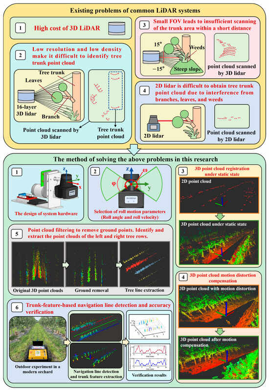
Figure 1.
Flowchart of the construction and evaluation of the 2D lidar-based perception system.
2.1. System Hardware Design
A customized orchard inspection robot, illustrated in Figure 2a, was employed as the mobile experimental platform. The robot boasts dimensions of 974.16 mm (length) × 782.02 mm (width) × 364 mm (height), featuring four 200 W servo motors for independent four-wheel drive capabilities with a maximum traveling speed of 0.5 m/s. These motors communicate with the lower computer via the RS485 protocol in a bus mode. The lower computer receives velocity commands sent by the industrial personal computer (IPC) and converts them into control signals to regulate the motor speed. Meanwhile, the lower computer can receive real-time encoder feedback from the motors, converting it into wheel speed, and transmits this information to the IPC through UART at a frequency of 50 Hz.
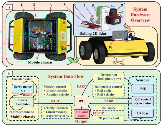
Figure 2.
System overview. (a) System hardware overview. 1. Servo motors (for driving wheels). 2. Lower computer. 3. Battery (48 V). 4. Voltage conversion modules. 5. DC motor driver. 6. Inertial Measurement Unit (IMU). 7. DC motor. 8. Servo controller (built-in magnetic encoder). 9. Two-dimensional lidar. 10. Industrial Personal Computer (IPC). All sensors and mechanical structures in this study follow a right-handed Cartesian coordinate system. Or-xyz represents the robot reference coordinate system, where the x-axis points in the direction of the robot’s forward motion, the y-axis points to the left of the robot’s forward direction, the z-axis points directly upwards from the robot, and the origin of this coordinate system is the projection point of the robot’s geometric center within the x-Or-y plane onto the ground. Ol-xyz is the reference coordinate system of 2D point clouds, whose origin is the center of the laser emitter, whose x-axis aligns with the optical axis of the 2D lidar. O3d-xyz denotes the reference coordinate system of constructed 3D point clouds, whose origin coincides with the origin of Ol-xyz, whose axes align with axes of Or-xyz and Oi-xyz (IMU coordinate system) (b) System data flow.
The robot is equipped with the designed rolling 2D lidar system, which mainly consists of a 6-axis IMU, a servo motor, and a 2D lidar, whose specific technical parameters are outlined in Table 1. The IPC commands the servo motor to roll the 2D lidar, registering each frame of 2D point clouds into the 3D space by utilizing the angle feedback of the servo motor. Moreover, the IMU and the wheel odometry are fused to estimate the system motion state for motion distortion compensation of the constructed 3D point cloud, which is then utilized for autonomous navigation tasks.

Table 1.
The main technical parameters of sensors utilized for rolling 2D lidar system.
2.2. Selection of the Roll Motion Parameters of 2D Lidar
In this study, the internal motion parameters of the rolling 2D lidar system primarily encompass the roll speed (ω) and angular range (φ). These two parameters directly determine the three core technical specifications of the system, namely the vertical field of view (V), the vertical resolution (R), and the roll scanning period (T). The equations for calculating these specifications are as follows:
where f is the scanning frequency of the 2D lidar, which is 30 Hz.
2.2.1. Two-Dimensional Lidar Roll Angle Selection
The selection of roll motion parameters for lidar not only needs to consider their impact on the quality of the 3D point cloud but also needs to be combined with the structural parameters of the orchard to ensure that the system can operate normally in the orchard environment. Therefore, this study surveyed the structural parameters of the Modern Apple Orchard of the National Apple Improvement Center located in Yangling District, Shaanxi Province, China. Figure 3a illustrates the inter-row structure of the orchard. The average row spacing between trees is approximately 4 m, and the plant spacing is about 1 m. The entire area between rows can be divided into three zones: A, B, and C. Zones A and C are the mulching areas at the base of the trees, which are inaccessible to robots, while zone B serves as the operational area for robots, allowing safe passage. Lines a and b are schematic navigation lines to guide the robot to travel along the centerline of the tree row and near one side of the tree row. Due to the constraints imposed by the mulching areas, the minimum distance that can be maintained between the center of the lidar and the single-sided tree row is approximately 0.95 m.
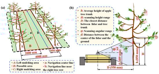
Figure 3.
Schematic diagram of roll motion parameters and modern orchard structural parameters (a) Modern orchard inter-row structural parameters. (b) Geometric relationship between roll angular range and fruit tree size parameters.
In semi-structured orchards, the tree trunk point cloud, being stable throughout seasons, pruning, and wind conditions, is typically extracted as the representation of the tree row, thereby acquiring the robot’s relative position within the inter-row space. Thus, the rolling lidar system must acquire sufficient 3D point clouds of trunks for robot inter-row positioning. As shown in Figure 3b, the installation height of the lidar’s optical axis center from the ground, denoted as d, is 489 mm, and the minimum distance to a single-sided tree row, denoted as D, is 950 mm. The average height of the fruit tree trunk region, denoted as h, is approximately 850 mm. Given the characteristic of the system’s vertical FoV, which exhibits a smaller vertical height at closer distances, it is necessary to select an appropriate roll angle range, denoted as φ, to ensure that when the robot travels along the navigation line b in Figure 3a, so the vertical FoV height H of the rolling lidar at a distance D from the tree row can adequately cover the trunk region. The calculation equation for H is
According to Equation (4), the final selected roll motion angle is 60°, and the vertical FoV height at a distance D is 1037.48 mm, which is sufficient to cover the entire trunk area of the fruit tree.
2.2.2. 2D Lidar Roll Velocity Selection
Given a fixed roll angle, the vertical resolution (R) and the scanning period (T) are uniquely determined by the roll velocity, and show a negative correlation, as can be inferred from Equations (2) and (3). Hence, it is significant to identify an appropriate rolling velocity that strikes a balance between resolution and scanning period. This velocity should ensure a dense point cloud, which is essential for accurate trunk detection while maintaining a reasonable scanning period crucial for real-time and stable navigation.
In terms of the scanning period, due to the continuous motion of the robot during a rolling cycle, by the time a frame of rolling scan is completed and the 3D point cloud is published, the lidar has already traveled a certain distance forward. This results in a spatial lag associated with the publication of each frame of the 3D point cloud. Therefore, to ensure the continuity and safety of autonomous navigation, the valid range of tree row point clouds in front of the lidar coordinate system origin, which is published at the end of the previous roll scanning cycle, must be no less than the distance traveled by the robot along the positive x-axis direction within one roll-scanning cycle.
Firstly, we embarked on an investigation into the maximum valid inter-row range that can be covered by each frame of the 3D point cloud under both static and continuous motion conditions of the system. To simplify the problem, we approximate the movement of the robot between fruit tree rows as a uniform linear motion along the positive direction of the x-axis. Furthermore, the valid region within the scanning range that can be used to fully describe the information of the fruit tree trunks between rows is approximated as an inscribed cuboid within the maximum area that can be covered by the 3D point cloud. To ensure comprehensive coverage of the orchard row width, the width of the cuboid is set to twice the orchard spacing. In the point cloud reference coordinate system, the y-coordinate range of the cuboid spans from −4 to 4 m, aligning with the orchard row width. Additionally, to ensure full coverage of the fruit tree trunk height along the z-axis, the height of the cuboid is designated as 1.2 m, with a z-coordinate range extending from −0.6 to 0.6 m.
Based on these assumptions, the task of determining the maximum length range of a tree row that can be covered by a single frame of 3D point cloud data can be simplified to calculating the maximum length (l) of the inscribed cuboid, along with its x-coordinate range (x1, x2), given the 3D point cloud acquired within a single rolling cycle, and the predefined width (w) and height (h) of the inscribed cuboid. In the static state of the system, the maximum coverage area of the point cloud within a single rolling cycle is represented by a part of a spherical cap, as illustrated by the orange area in Figure 4a. In this case, the maximum length of the inscribed cuboid and its x-coordinate range can be calculated as follows:
where represents the detection range of the 2D lidar, specifically 25 m, while denotes the horizontal FoV of the 2D lidar, which measures 270°. The result is shown as the blue cuboid in Figure 4a.
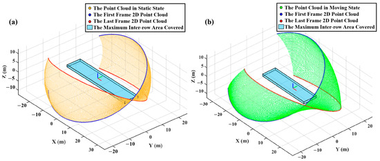
Figure 4.
Schematic diagram of the maximum coverage range of the 3D point cloud and the maximum area that the tree row can be covered under static and moving states. (a) The maximum area covered by the point cloud generated by the system in a stationary state during one roll cycle, as well as the maximum area within the point cloud that can include the trunk area of fruit trees in the current tree row. (b) The maximum area covered by the point cloud generated by the system in a moving state during one roll cycle, as well as the maximum area within the point cloud that can include the trunk area of fruit trees in the current tree row.
As for the system in the motion state, the maximum coverage range of a 3D point cloud is an irregular surface, as shown in the green area in Figure 4b, making it difficult to obtain its maximum inscribed cuboid. Therefore, this study adopts a conservative and simplified approach to calculate the length () and the x-coordinate range () of the inscribed cuboid. Specifically, the and can be calculated based on the intersection of the two spherical caps where the curves of the maximum scanning range of the 2D point cloud in the first and last frames of a rolling cycle are located.
where v represents the robot movement speed and T is the roll period.
Secondly, according to Equations (3) and (9), it can be seen that when the roll angle is determined, the effective forward distance of the 3D point cloud obtained in the moving state is determined by both the roll velocity (ω) and the robot movement velocity (v). The smaller the ω and the larger the v, the shorter the will be, making it more difficult to meet the system requirements. However, a too-large value of ω will reduce the vertical resolution of the 3D point cloud, thereby affecting the tree trunk detection based on the point cloud. In addition, a too-small value of v will result in autonomous navigation not meeting the speed requirements of orchard operations. To settle this problem, we have firstly limited the range of robot movement speed. At present, most autonomous robot systems used in orchards for precision agricultural tasks (phenotype analysis, picking, pruning, etc.) typically move at a speed of no more than 1 m/s [24,25,26,27]. Considering that the maximum traveling speed of the mobile chassis used in this article is 0.5 m/s, and to ensure the safety redundancy of the system, this study uses 1 m/s as the limiting condition to select the roll velocity that meets the system requirements, which is shown as follows:
where vmax denotes the maximum moving speed of the robot, specifically 1 m/s.
Ultimately, the minimum roll speed calculated to meet the system requirements is 4.863°/s. In this state, the maximum coverage area of the intra-row fruit tree trunks by the continuously generated 3D point clouds during the uniform linear motion of the robot is shown in Figure 5. The lidar coordinate system is utilized as a reference, with the lidar starting from point O and traveling along the positive direction of the x-axis at a speed of 1 m/s. When the lidar reaches point O1, it completes the first roll cycle scan and publishes orange 3D point cloud data, fully covering the trunks of fruit trees within the blue cuboid region. As the lidar moves to the end of the blue cuboid at O2, the system completes the second roll scan cycle and publishes green point cloud data, supporting autonomous navigation for the subsequent scan cycle.
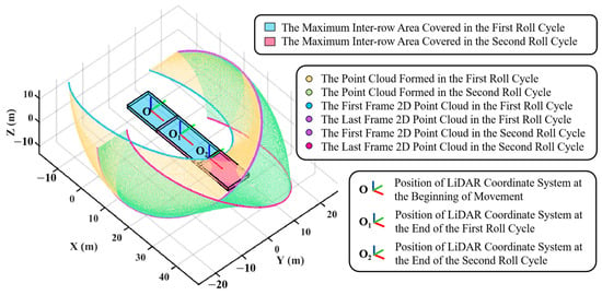
Figure 5.
Maximum coverage area of two consecutive 3D point clouds generated during two consecutive roll cycles when the robot moves at a constant speed of 1 m/s in a straight line, and the lidar rolls at a minimum speed of 4.863°/s between −30° and 30°, including the region that fully encompasses the main trunk of the fruit trees within the row.
Moreover, to ensure the spatial distribution uniformity and high resolution of the 3D point cloud, this study uses 0.25°, which is the same as the horizontal resolution, as the vertical resolution of the system. By substituting it into Equation (2), the calculated value is 7.5°/s, which meets the system requirement. The final determined motion parameters of the system are φ = 60° and ω = 7.5°/s.
2.3. Registration of 2D Point Clouds to 3D Point Clouds
Under a static state, the robot does not generate external motion, and the internal motion of the system is only the periodic roll motion of the 2D lidar around the output axis of the servo motor. At this time, the principle of projecting the 2D point cloud into 3D space is shown in Figure 6. First, the initial 2D point cloud obtained by the lidar is converted from the polar coordinate system to the Cartesian coordinate system by Equation (12):
where (, , ) is a point in the Cartesian coordinate system, while and are, respectively, the range measurement of the point by the lidar in the polar coordinate system and the current angle of the lidar rotating mirror.
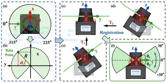
Figure 6.
Schematic diagram of converting the 2D point cloud to the 3D point cloud. (a) The 2D lidar coordinate system and the 2D scanning range. (b) Schematic diagram of converting the 2D point cloud from a polar to Cartesian coordinate system. (c) Initial lidar coordinate system before rotation, aligning with the 3D point cloud reference coordinate system (O3d-xyz). (d) The 2D point cloud data in O2-xyz after clockwise rotation of O-xyz around the x-axis by θ2. (e) The 2D point cloud data in O1-xyz after anticlockwise rotation of O-xyz around the x-axis by θ1. (f) Registration of the 2D point clouds from O1-xyz and O2-xyz with T1 and T2 coordinate transformations to generate 3D point cloud data in O3d-xyz.
Subsequently, as shown in Figure 6c–f, the 2D point cloud in the lidar coordinate system Ol-xyz is registered to the 3D point cloud reference coordinate system O3d-xyz. In the ideal state where the motor output axis coincides with the lidar optical axis, the angle (θi) fed back by the motor encoder is the rolling angle of Ol-xyz around the x-axis of O3d-xyz. Therefore, the coordinates of 3D point clouds () can be obtained through Equation (13):
However, since the lidar and encoder employ distinct clock control sources, and their data transmission frequencies are different at 30 Hz and 180 Hz, respectively, a software-level time synchronization is conducted to ensure that the lidar data syncs with the roll angle fed back by the encoder when projecting it into the 3D space. The specific implementation process is illustrated in Figure 7. Finally, the system is calibrated using the method proposed by Hatem Alismail and Brett Browning [28] to eliminate the point cloud distortion caused by assembly errors.
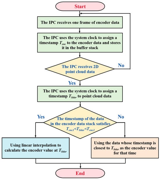
Figure 7.
Flowchart of time synchronization between lidar and encoder.
The linear interpolation (LERP) equation is
where represents the angle of encoder feedback after time synchronization with lidar data. Tlidar is the timestamp of the 2D lidar data, while and denote the timestamps of data in the encoder data stack that are closest to Tlidar and are, respectively, less than and greater than Tlidar. and represent the roll angle values measured by the encoder at and , respectively.
2.4. Motion Distortion Compensation of the 3D Point Cloud
When the system is in a motion state, the 3D point cloud calculated directly by Equation (13) will show severe distortion in a relatively long rolling cycle without knowing the system motion state. Therefore, real-time accurate system motion state estimation is of great significance for compensating for the motion distortion of the 3D point cloud and ensuring the safety and stability of autonomous navigation. A combination of wheel odometry and IMU was employed to achieve 6 Degree of Freedom (6-DOF) motion state estimation for the rolling lidar system to eliminate the point cloud motion distortion. In this study, the reference coordinate system for 3D point clouds is set as O3d-xyz, and all processing related to 3D point clouds is completed within this reference coordinate system. Therefore, the core steps for estimating the system’s motion state include, firstly, establishing the initial state coordinate system O3d-xyz at time zero as the global coordinate system, and secondly, obtaining the real-time coordinate transformation of O3d-xyz relative to this global coordinate system after time zero. The pipeline of 3D point cloud motion distortion compensation is shown in Figure 8.
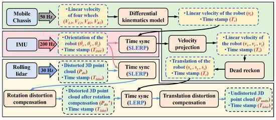
Figure 8.
Pipeline of motion distortion compensation of the 3D point cloud using wheel odometry and IMU.
The system can continuously obtain the speed of the four wheels from the chassis at a frequency of 50 Hz. In addition, due to the slow movement speed of the robot (maximum speed of 0.5 m/s) and the fact that the error of the odometry only accumulates in one rolling cycle (8 s) and is updated in the next cycle, the slip and speed jump of the wheel odometry in one rolling cycle can be ignored in this study. Therefore, the kinematics of the robot can be simplified as a differential model, as shown in Figure 9a. Specifically, the linear velocity vr and angular velocity ωr of the robot can be calculated as follows:

Figure 9.
Schematic diagram of 6-DOF pose estimation based on IMU and wheel odometry. (a) Principle of wheel odometry based on differential model and schematic of the additional translation [∆x, ∆y, 0]T between O3d′-x′y′z′ and O3d″-x″y″z″ caused by spatial offset x3d2r between Or-xyz and O3d-xyz in the x-O-y plane. (b) Schematic of the displacement along the z-axis calculated by combining wheel odometry and IMU.
Nevertheless, the velocity vector [vr, ωr]T can only calculate the 2D motion state in the x-O-y plane, but in the actual orchard environment, there are significant ground undulations, as shown in Figure 9b. Therefore, this study uses the orientation information obtained from IMU to project the linear velocity of the robot into 3D space and integrates the velocities in the three-axis directions to calculate the 3D translation of the robot’s coordinate system Or-xyz relative to its initial motion state:
where represents the rotation matrix of the robot at and [, , ]T represents the linear velocity components of the robot along the x, y, and z axes at ti. [sx(ti), sy(ti), sz(ti)]T is the translation vector of the robot at ti. To ensure the synchronization of sensor data during velocity projection, the timestamp of the wheel odometry ti is used as the reference time, and spherical linear interpolation (SLERP) is utilized to obtain the synchronized orientation value of the IMU at ti.
Subsequently, the translation vector of O3d-xyz is required to compensate for the 3D point cloud distortion caused by translation. However, due to the spatial offset between the Or-xyz coordinate system and the O3d-xyz coordinate system, additional displacement is added to the O3d-xyz coordinate system when the robot undergoes rotation. For instance, as illustrated by the light blue sector in Figure 9a, the rotation of Or’-x’y’z’ around its own z-axis results in the translation [∆x, ∆y, 0]T between O3d’-x’y’z’ and O3d”-x”y”z”. Therefore, it is necessary to convert the translation of the robot coordinate system Or-xyz relative to its initial state into the translation of the O3d-xyz coordinate system relative to its initial state using the following equations:
where [x3d2r, y3d2r, z3d2r]T denotes the offset between Or-xyz and O3d-xyz, [∆x, ∆y, ∆z]T represents the additional translation of O3d-xyz caused by the rotation of the robot, and T(ti) is the translation vector of O3d-xyz at ti.
Due to the rigid connection between the rolling lidar system including IMU and the mobile chassis, the rotation state of the coordinate system O3d-xyz is the same as the orientation output of IMU. Therefore, the IMU data synchronized with the lidar data by using SLERP are directly employed to compensate for the 3D point cloud distortion caused by rotation. Similarly, the 3D point cloud distortion caused by translation is also corrected by the synchronized translation vector T(ti):
where [, , ]T represents the distorted 3D point cloud at , while [, , ]T represents the undistorted 3D point cloud after correction at , and and represent the rotation matrix and the translation matrix, respectively, of the O3d-xyz coordinate system at .
2.5. Navigation Line Extraction Based on 3D Point Clouds
In Section 2.4, the 3D point cloud data obtained not only include information about the tree row but also contain data from adjacent tree rows, branches, weeds, and a significant amount of ground points. This not only greatly increases the data volume, reducing computational efficiency, but also introduces noise that severely affects the extraction of tree row point clouds and the fitting of navigation lines. To address these issues, this study developed a navigation-line-detection strategy by fusing geometric features of trunks and RANSAC, as shown in Figure 10.
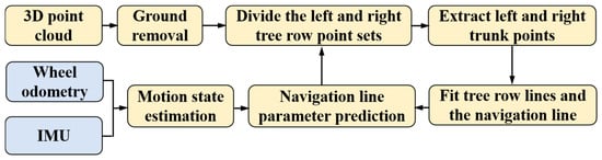
Figure 10.
Navigation line extraction pipeline.
2.5.1. Tree Row Point Cloud Segmentation
For removing ground point clouds, the uneven terrain and slope of the orchard floor make it difficult to effectively distinguish between ground and tree row point clouds using a simple passthrough filter based on the z-axis coordinates. Additionally, the RANSAC plane fitting method struggles to handle non-planar areas with significant height variations and is computationally inefficient. To ensure effective ground point segmentation and real-time algorithm performance, this study adopts the Patchwork algorithm proposed by Hyungtae Lim et al. [29]. The algorithm consists of three main components: Concentric Zone Model (CZM), Region-wise Ground Plane Fitting (R-GPF), and Ground Likelihood Estimation (GLE). The CZM first spatially divides the point cloud into concentric annular sectors centered at the origin of O3d-xyz. This allows for plane fitting of the ground points within each subset, addressing the issues of terrain undulation and uneven point cloud distribution. Next, the R-GPF utilizes Principal Component Analysis (PCA) to perform ground plane fitting within each grid interval, selecting potential ground point candidates. Finally, the GLE applies a region-based binary classification probability test to enhance the accuracy of ground point identification and extract the final ground point cloud.
Subsequently, a point cloud filtering method is proposed, as illustrated in Figure 11, to ensure that the filtered 3D point cloud can fully cover the information of the current row, and filter out point cloud data from the vehicle body and adjacent tree rows, effectively distinguishing between the left and right tree row point clouds. Firstly, taking O3d-xyz as the reference coordinate system, based on the geometric dimensions of the robot, a pass-through filter is employed to remove the point cloud of the vehicle body. Secondly, addressing the issue where the rapid rotation of the robot within a short period leads to misalignment between the tree row distribution and the robot travel direction, making it difficult to filter out adjacent tree row point clouds via pass-through filtering and distinguish between left and right point clouds, this study utilizes the tree row centerline lo detected from the previous frame point clouds, combined with robot motion state, to predict parameters of centerline lp for the current frame’s point cloud. Assuming that the position and direction of a straight line can be expressed using the coordinates of two points p1(0, b) and p2(1, k + b) on the line, lo can be represented by (0, bo) and (1, ko + bo), where ko and bo are the slope and intercept of lo, respectively. The line parameters of lp can be obtained using Equation (23):
where (, , ) represents the change of the robot motion state in the xy plane from the previous point cloud observation moment to the current moment. The and are the slope and intercept of lp, respectively. Finally, the point cloud data on both sides of lp, which are within a distance of less than Wtr from the line, are extracted separately as the left and right tree row point cloud sets.
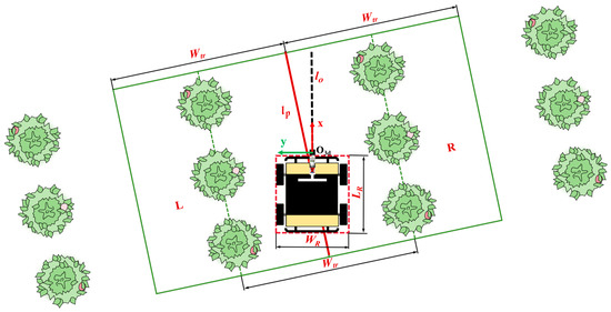
Figure 11.
Schematic diagram of point cloud filtering and point set division. The red dashed rectangle is the passthrough filter area for vehicle points removal, where WR and LR are the width and length of the vehicle, respectively. The green rectangles L and R are the regions for left and right tree row extraction, where Wtr is the width of the tree row. The black dashed line lo is the mid-line detected in the previous frame of point cloud. The red line lp is the mid-line predicted by lo and the robot motion state.
2.5.2. Navigation Line Extraction Based on Geometric Features of Trunks and RANSAC
In Section 2.5.1, the point clouds obtained from the left and right tree rows still contain residual ground points, as well as a significant amount of lateral branches and foliage clusters. Therefore, it is necessary to further extract the trunk point clouds that can stably represent the tree rows. The trunk structure in modern orchards is shown in Figure 12a, where, compared to foliage and ground points, the trunk exhibits distinct geometric characteristics that can be approximated as a cylinder approximately parallel to the z-axis of the reference coordinate system O3d-xyz. Based on these features, this study employs PCA to extract the local geometric features of the point clouds. Taking a local point cloud set as an example, each data point pi is a three-dimensional vector containing the (x, y, z) coordinates of the point cloud. Firstly, the mean vector of the samples is calculated, as shown in Equation (26):
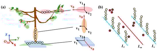
Figure 12.
Trunk point extraction and navigation line detection. (a) Point cloud local geometric feature extraction, where (v0, v1, v2) are the first three eigenvectors of the local point cluster. (b) Navigation line fitting based on RANSAC. Red points represent the outliers, while yellow points are the inliers. Ll, Lm, and Lr represent the left tree row line, the tree row midline, and the right tree row line, respectively.
Subsequently, the dataset is centered using the mean vector:
Then, the covariance matrix Cov is calculated for the centered dataset:
By performing eigenvalue decomposition on the covariance matrix, the top three eigenvalues (λ0, λ1, λ2) and their corresponding eigenvectors (v0, v1, v2) are obtained. The eigenvector v0 corresponding to the largest eigenvalue λ0 represents the direction of maximum variance distribution in the point cloud dataset. As shown in Figure 12a, compared to the ground and foliage, the principal eigenvector of the tree trunk is approximately parallel to the z-axis of the O3d-xyz coordinate system. Based on this geometric constraint, this study first employs the K-D tree to perform nearest neighbor search for each data point. Subsequently, the principal eigenvector for each point is computed based on its neighboring points. Points whose principal eigenvectors form an angle with the z-axis of the O3d-xyz coordinate system that is bigger than a specified angular threshold are filtered out, thereby extracting point cloud data that are more highly correlated with the tree trunk.
After the above operations, most of the point cloud that does not belong to the tree trunk has been filtered out, but there are still a small number of side branches and weeds whose main directions are approximately perpendicular to the ground, which can act as noise information during the detection of tree rows, as shown by the red points in Figure 12b. Therefore, the RANSAC algorithm is utilized for line fitting. Through iterative cycles of sampling, modeling, and evaluation, it selects inliers that best represent the tree row information. Since fruit trees in modern orchards are planted in straight rows, this geometric constraint helps further extract the tree trunk point cloud during the inlier selection process within RANSAC. Taking the point cloud Ql on the left side as an example, since the fitting of the navigation line is a 2D problem in the xy plane, only the x and y coordinates of the point cloud data in Ql are extracted to construct a new point set Ql’. From this, two points p1(x1, y1) and p2(x2, y2) are randomly selected to calculate the line parameters:
For the remaining points (xi, yi) in Ql′, the distance di of each point to the current line is calculated:
Compare di with the distance threshold dthreshold, and define all points with distances less than dthreshold as inliers and store them in the inlier set Qin. Then, continue to repeat the above steps. When the number of inliers corresponding to a line model exceeds the number of inliers obtained from the previous calculation, update the model parameters and the inlier set. After meeting the condition for the number of iterations, select the line parameters corresponding to the largest number of inliers as the output. Apply the above method for line fitting to the left and right point clouds separately, and extract the parametric representations (kl, bl) and (kr, br) for the left and right tree rows, respectively. The red navigation line in Figure 12b can be obtained by averaging the parameters of the left and right tree rows:
3. Results
3.1. Assessment of Rolling 2D Lidar System Performance
3.1.1. Results of Point Cloud Registration
In this study, we conducted both an indoor experiment and an outdoor experiment to test the effectiveness of the 3D point cloud construction. The indoor experiment was primarily used for calibrating the internal parameters of the system to eliminate point cloud distortion caused by assembly errors. Since the calibration algorithm constructs the loss function based on the distance from a point to a plane, an indoor environment with abundant planar features was selected as the test site. Initially, the servo motor was controlled to rotate a full revolution at a speed of 27.5°/s, ensuring that the angle feedback values were synchronized with the lidar data using the method outlined in Section 2.3. Subsequently, the data collected in the full revolution were utilized for calibration. The 2D lidar in a full revolution can scan the same environment two times: the first half (0–180°) and the second half (180–360°). However, as shown in Figure 13b, the assembly errors prevent the two point sets from overlapping. This misalignment is particularly evident in enlarged views 1 and 2, where significant deviations can be clearly seen between the screens, tables, and corners of the walls within the two point sets. The result shows that after 13 iterations, the rotational and translational deviations between the two point clouds converged from the initial values of 1.293° and 13.1 mm to 6.749 × 10⁻⁵° and 3.816 × 10⁻⁴ mm, respectively. The final calibration result is illustrated in Figure 13b. As evident from enlarged views 1 and 2, the calibrated point sets overlap well, displaying clear environmental structural information and contour details.
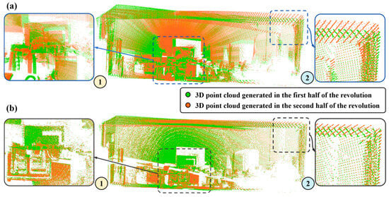
Figure 13.
Comparison results before and after internal parameter calibration. (a) The 3D point cloud of the laboratory generated in the first and the second half of the revolution before calibration. 1. The enlarged view of the uncalibrated 3D point cloud of the screen and the desk. 2. The enlarged view of the uncalibrated 3D point cloud of the corner of the walls. (b) The 3D point cloud of the laboratory generated in the first and the second half of the revolution after calibration. 1. The enlarged view of the calibrated 3D point cloud of the screen and the desk. 2. The enlarged view of the calibrated 3D point cloud of the corner of walls.
The outdoor test was conducted at a modern apple orchard in Yangling District, Shaanxi Province, China. As shown in Figure 14a,b, the robot was, respectively, placed at point a on the centerline of the tree row and point a’ on the guidance line indicating the closest distance (0.95 m) in which the robot can maintain with a single row of trees, as measured in Section 2.2.1, to acquire static 3D point clouds of fruit trees.
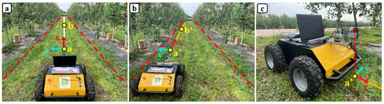
Figure 14.
Outdoor test scenario. (a) Experimental scenario where the robot is located at the centerline of a tree row, where points a, b are nearly at the head and end of the tree row. (b) Experimental scenario where the robot is close to the left tree row, where points a’, b’ are at the head and end of the tree row. (c) Point a’ is the projection of the rolling lidar coordinate system origin on the ground plane (x-O-y-plane).
The 3D point cloud obtained by the rolling 2D lidar system under a static state is shown in Figure 15. Figure 15a is a top view of the orchard 3D point cloud obtained when the robot is placed at point a. The left tree row point cloud detail in the blue dashed box is shown in Figure 15b, while its right counterpart in the yellow dashed box is shown in Figure 15c. Owing to the similar distance between the lidar and two tree rows, point clouds acquired from both sides have almost the same density. Furthermore, it can be demonstrated that the point cloud has sufficient vertical FoV to fully cover the trunk areas and can also clearly display the geometric details of fruit tree trunks. Additionally, Figure 15d–f depict the top view and enlarged view of the left and right tree row 3D point cloud data collected by the robot at point a’. Due to the proximity of the lidar system to the left tree row and its inherent characteristics of generating dense point clouds with narrow vertical coverage in close proximity and sparse point clouds with wide vertical coverage at greater distances, it is evident that the vertical coverage of the fruit tree trunk in Figure 15e is narrower than that in Figure 15f. Furthermore, the point cloud density in Figure 15f is notably lower. Despite these differences, both Figure 15e,f demonstrate an adequate quantity, completeness, and clarity of the fruit tree trunk point clouds for autonomous navigation, thereby reinforcing the validity of the system parameter design outlined in Section 2.2.
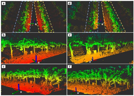
Figure 15.
The 3D point cloud of the orchard, indicating varying heights through color, collected at observation points a and a’ under the static state. (a) The top view of both the left and right tree row point cloud at a. (b) The enlarged view of the left tree row point cloud at a. (c) The enlarged view of the right tree row point cloud at a. (d) The top view of both the left and right tree row point cloud at a’. (e) The enlarged view of the left tree row point cloud at a’. (f) The enlarged view of the right tree row point cloud at a’.
Additionally, a comparison between the rolling 2D lidar and three different common commercially available 3D lidars is shown in Table 2, so as to demonstrate the quality of the 3D point cloud obtained by the rolling 2D lidar, as well as its cost-effectiveness. It can be seen that compared to the three types of lidars—C16, C32, and OS1-128—the system proposed in this paper exhibits higher vertical resolution and a larger vertical FoV. Moreover, its price is far lower than those of several other commercial lidar options. (Note: The Rolling 2D lidar system proposed in this research offers these advantages primarily in low-speed orchard operation scenarios. However, in high-speed and complex operational scenarios such as urban autonomous driving, its ranging capability and update frequency are insufficient to support normal operation.)
Table 2.
The main technical parameters and prices of common commercially available 3D lidar and the rolling 2D lidar system.
3.1.2. Results of the Point Cloud Motion Distortion Compensation
To verify the compensation effect of point cloud motion distortion, the robot was controlled to travel at the highest speed (0.5 m/s) from point a to point b along the white navigation line in Figure 14a. At point b, the robot saved the 3D point cloud data published at this time and stopped moving. The results of point cloud motion distortion compensation are shown in Figure 16, where Figure 16a is the 3D point cloud data of the left tree row obtained by the robot at a speed of 0.5 m/s from point a to point b without motion distortion compensation. It can be observed that the point cloud has extremely severe distortion, making it difficult to identify the point cloud of trunks. On the other hand, Figure 16b illustrates the 3D point cloud of the same tree row in Figure 16a after motion distortion compensation. It is evident that the motion distortion on the point cloud is remarkably eliminated, and the surface contours of the tree trunks are dramatically clear, which is convenient for the recognition and positioning of tree trunks, thus ensuring the reliability of autonomous navigation. This demonstrates that the point cloud motion distortion compensation method proposed in this study can achieve good correction effects for linear motion distortions within 0.5 m/s.
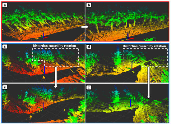
Figure 16.
Results of the 3D point cloud motion distortion compensation, where colors represent variations in height. (a) The 3D point cloud of the left tree row with distortion caused by a motion speed of 0.5 m/s. (b) The 3D point cloud of the left tree row after motion distortion compensation at 0.5 m/s. (c) The 3D point cloud at the end of the tree row with distortion caused by a U-turn operation. (d) The next frame of the point cloud in Figure (c) shows distortion caused by a U-turn operation. (e) The 3D point cloud at the end of tree rows after motion distortion compensation during the U-turn operation. (f) The next frame of the point cloud in Figure (e) after motion compensation.
Additionally, to validate the system’s capability in correcting point cloud distortion caused by large-scale rotation, we remotely controlled the robot to execute a U-turn operation at the end of the tree row, simulating the actual conditions during autonomous navigation. Figure 16c,d show the two consecutive frames of 3D point cloud data captured during the turning process. It is evident that significant rotational motion introduces more severe distortion to the point cloud of objects located further away from the rotation center of the vehicle, as exemplified by the point clouds enclosed within the white dashed boxes in Figure 16c,d. Moreover, in Figure 16e,f, the severe distortions present in these two frames of point clouds have been significantly corrected, allowing the fruit tree trunks to be clearly discerned.
Overall, the 3D point cloud motion compensation method proposed in this study has successfully achieved compensation for point cloud motion distortion during the intra-row travel and the U-turn operation, ensuring the quality and validity of the point cloud acquired by the system throughout the entire navigation process.
3.2. Assessment of Navigation Line Detection
3.2.1. Results of the Tree Row Point Cloud Extraction
To verify the effectiveness of the method described in Section 2.5.1 for filtering and extracting tree row point clouds, this study conducted an outdoor test in the modern orchard. The real-time effects of point cloud processing were continuously observed by remotely controlling the robot to travel from the beginning to the end of a tree row. The results are shown in Figure 17a–c. By comparing (a) and (b), it can be seen that the patchwork algorithm successfully filters out the uneven ground points and extracts all the tree row point clouds. By comparing (b) and (c), it is evident that utilizing the predicted centerline parameters enables the successful extraction of the point cloud of the current tree row where the robot is located and distinguishes between the left and right tree rows. To further validate the filtering performance of the centerline-prediction-based filtering method for the left and right tree row point clouds when the robot undergoes large-scale rotation within the tree row, the robot was controlled to rapidly rotate toward the left tree row from a point on the centerline, and its filtering effect was observed, as shown in Figure 17d–f. It can be seen that even under large-scale rotation, the tree row extraction method proposed in Section 2.5.1 can still successfully extract and distinguish the tree row point clouds on both sides of the robot.
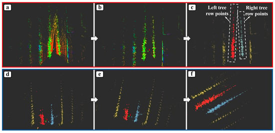
Figure 17.
Filtering results of tree row point clouds. (a) Original 3D point clouds, indicating varying heights through color. (b) Three-dimensional point clouds after ground removal, indicating varying heights through color. (c) Extraction and distinction of point clouds from the left and right adjacent tree rows for the robot. The red point cloud within the left white dashed box represents the left tree row, while the blue point cloud within the right white dashed box represents the right tree row. The yellow point cloud represents point clouds outside the current tree row. (d) Segmentation result of point clouds from the left and right tree rows when the robot is at a certain point on the centerline within the row. (e) Segmentation result of point clouds from the left and right tree rows during the robot rotation. (f) Segmentation result of point clouds from the left and right tree rows when the robot stops alongside the left tree row after completing its rotation.
3.2.2. Results of Navigation Line Detection
In this study, the same outdoor test as described in Section 3.1.1 was employed to control the robot to travel along the centerline from the beginning to the end of the row, with an analysis of the effectiveness of point cloud trunk extraction and navigation line fitting during the movement. Taking Figure 18 as an example, (a) depicts the point clouds of the left and right tree rows extracted by the point cloud filtering module. It can be observed that the point clouds still contain a significant amount of noise points beyond the tree trunks, such as residual ground points, orchard display boards, and numerous branches and leaves. By comparing (a) and (b), it can be seen that after segmenting the point clouds using their local geometric features, the remaining ground points display board point clouds, and some of the disorderly lateral branches of the fruit trees are removed, making the point clouds of the trunk area clearer and more prominent. However, there are still many noise point clouds from the canopy and lateral branch areas. By comparing (b) and (c), it can be observed that when using RANSAC for tree row line fitting, the geometric constraints based on the linear distribution of the tree rows enable RANSAC to further extract the point clouds of the trunk area during the process of selecting inliers.
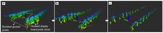
Figure 18.
Results of point cloud segmentation for fruit tree trunks, where colors represent variations in height. (a) Unprocessed point clouds of the left and right tree rows, where the point clouds in the white dashed region are residual ground points, and the rectangular-shaped point clouds in the right tree row represent display boards in the orchard. (b) Tree row point clouds after segmenting the point clouds in (a) using local geometric features. (c) Inliers extracted by RANSAC from the point clouds in (b).
The results of tree row detection are shown in Figure 19. From (a), it can be observed that directly applying RANSAC line fitting to the left and right tree row point clouds results in significant influence from noise data within the tree row point clouds, leading to extracted tree row lines that do not align with the actual tree row distribution, and the left and right lines are severely non-parallel. However, if the point clouds are initially constrained using local geometric features to remove most of the excess noise data, followed by RANSAC for line fitting, better tree-row-detection results can be obtained, as shown in (b). The left and right tree rows are not only parallel but also highly consistent with the actual tree row distribution. Further analysis of the inliers extracted by RANSAC in (a) reveals that, as seen in (c), when the side branches and leaves in the tree rows are very dense and the point cloud number and density exceed that of the trunk, RANSAC tends to extract these parts of the point cloud as inliers, making it difficult to extract feature points that truly represent the tree row position and direction. In contrast, (d) first constrains the point cloud data in the z-axis direction using local geometric features, screening out candidates that are more likely to be from the tree trunk. Subsequently, RANSAC is used to constrain the point cloud along the tree row direction, further extracting potential trunk point clouds of the fruit trees, which can more stably represent the tree rows.
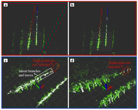
Figure 19.
Tree-row-detection results: (a) Results of directly applying RANSAC for tree row detection to the left and right tree row point clouds. (b) Results of tree row detection using a combination of local geometric feature constraints and RANSAC. (c) Inliers extracted directly from the tree row point clouds using RANSAC, where the white point cloud represents inliers, the green point cloud represents outliers, and the point clouds within the white boxes are those that are actually side branches and leaf points but have been incorrectly detected as inliers; the point clouds within the red boxes are those that are actually trunk points but have not been recognized as inliers. (d) Inliers extracted using a combination of local geometric feature constraints and RANSAC, where the white point cloud represents inliers, the green point cloud represents outliers, and the point clouds within the red boxes are trunk points that were not detected in (c) but are now correctly identified as inliers.
To verify the accuracy of the extracted navigation line, this experiment collected real-time 3D point cloud data constructed as the robot traveled between rows in the orchard. The point cloud of the tree trunk area was manually labeled and extracted using the Point Cloud Toolbox in Matlab. Subsequently, a navigation line was fitted based on the extracted trunk points as the ground truth. This was compared with the navigation line obtained using the method proposed in Section 2.5. The accuracy of the navigation line was evaluated using the angle and distance errors between the output and the ground truth. The angle error was directly calculated using the slopes. The distance error was determined by uniformly discretizing the line into 1000 points within a line segment from 0 to 10 m on the x-coordinate and calculating the average distance of these points to the ground truth. Furthermore, to verify the robustness of the navigation-line-detection module proposed in this study under different moving speeds, the robot was controlled to move between the rows in an orchard at speeds of 0.2 m/s and 0.5 m/s (the maximum moving speed of the robot), respectively. The evaluation method mentioned above was then employed to validate the accuracy of the navigation line at these different moving speeds.
As shown in Figure 20a,b, when the robot operates at a speed of 0.2 m/s, the maximum angular error between the navigation line extracted by the algorithm and the ground truth does not exceed 0.6°, with an average angular error of 0.272°. The maximum distance error does not exceed 0.05 m, and the average distance error is 0.023 m. When the robot moves at a speed of 0.5 m/s, it reaches the end of the row by the 16th frame. Therefore, Figure 20c,d illustrate the accuracy of the navigation line for the first 16 frames at a moving speed of 0.5 m/s. The maximum angular error of the navigation line does not exceed 0.6°, with an average angular error of 0.146°. Additionally, the maximum distance error does not exceed 0.055 m, and the average distance error is 0.016 m, demonstrating the same level of navigation line accuracy as when moving at 0.2 m/s.
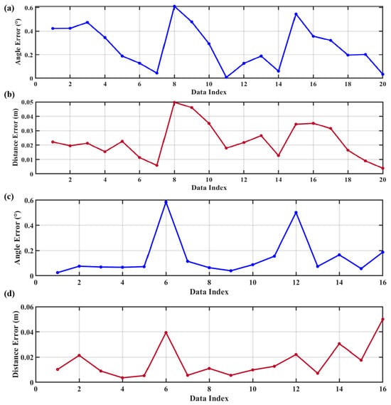
Figure 20.
Results of detected navigation line accuracy verification. (a) Navigation line angle error at a moving speed of 0.2 m/s. (b) Navigation line distance error at a moving speed of 0.2 m/s. (c) Navigation line angle error at a moving speed of 0.5 m/s. (d) Navigation line distance error at a moving speed of 0.5 m/s.
The above results demonstrate that the navigation-line-detection algorithm based on 3D point clouds proposed in this research can achieve high-accuracy perception to guide the robot to move safely within the rows. Moreover, the system exhibits good performance at different moving speeds, further indicating that the system possesses high robustness under various speed conditions.
3.2.3. Verification of the Impact of Different Rolling Motion Parameters on Navigation-Line-Detection Performance
To further verify the rationality of the rolling motion parameters identified in Section 2.2 and their impact on the effectiveness of navigation line detection, with reference to the vertical FoV of 30° and vertical resolution of 2.0° for the LeiShen C16 lidar (which, in the context of this study, corresponds to a rolling angle of 30° and a rolling velocity of 60°/s for the rolling 2D lidar), the study combines different rolling angle ranges (30°, 60°) with rolling velocities (7.5°/s, 60°/s) into four scenarios. The robot with the four different parameter combinations is controlled to navigate within the same orchard row, and the navigation line fitting results are output in real time using the method described in Section 2.5. The same method for navigation line accuracy verification outlined in Section 3.2.2 is adopted, comparing against the manually labeled ground truth to investigate the influence of different rolling motion parameters on navigation-line-detection accuracy. Table 3 presents the average distance error and average angular error of the system’s navigation line detection under the four different combinations. Among them, when the system’s vertical FoV is 30° and the vertical resolution is 2.0°, the average angular error and average distance error of the navigation line are the largest, at 0.814° and 0.065 m, respectively. Additionally, when the system’s vertical FoV is 30° and the vertical resolution is 0.25°, the average angular error and average distance error of the navigation line are the smallest, at 0.198° and 0.018 m, respectively.
Table 3.
The average angular error and average distance error of the extracted navigation lines under four different combinations of vertical FoV and vertical resolution.
Under the condition of a fixed vertical resolution in the system, the impact of vertical FoV on the accuracy of navigation line detection is compared. When the vertical resolution is 2.0°, the accuracy of navigation lines is relatively low for both 30° and 60° vertical FoVs. Furthermore, as the vertical FoVs increase from 30° to 60°, there is a slight improvement in the accuracy of navigation line detection. Additionally, when the vertical resolution is 0.25°, the accuracy of navigation lines is relatively high for both 30° and 60° vertical FoVs. In this case, there is a slight decrease in navigation line accuracy when the vertical FoVs increase from 30° to 60°. Based on this analysis, when the system’s vertical FoV is no less than 30°, the accuracy of the navigation line is not sensitive to changes in the vertical FoV.
Similarly, when the system’s vertical FoV is fixed, the impact of vertical resolution on the accuracy of navigation line is compared. When the vertical FoV is set at 30° and the vertical resolution is increased from 2.0° to 0.25°, there is a significant improvement in the accuracy of navigation line detection. Specifically, the average angular error and average distance error decrease from 0.814° and 0.065 m to 0.198° and 0.018 m, respectively. Likewise, when the system’s vertical FoV is 60° and the vertical resolution is increased from 2.0° to 0.25°, the average angular error and average distance error of the navigation-line-detection results rapidly decrease from 0.681° and 0.059 m to 0.272° and 0.023 m, respectively. These results demonstrate that within the range of 0.25° to 2.0°, the vertical resolution has a substantial impact on the accuracy of navigation line detection in the system, indicating that a higher vertical resolution leads to higher accuracy in navigation line detection.
Figure 21 demonstrates the impact of different combinations of vertical FoV and vertical resolution on the accuracy of navigation line detection during the entire movement of the robot. In Figure 21a,b, it is evident that when the system’s vertical FoV is 30° and the vertical resolution is 2.0°, there is a significant error in the navigation-line-detection result of the third frame (with an angular error of 5.815° and a distance error of 0.404 m). Figure 21c displays the navigation-line-detection results of the third frame and the extraction of tree trunk feature points under four combinations of system parameters. The figure in the upper left orange box shows the navigation-line-detection result when the system’s vertical FoV is 30° and the vertical resolution is 2.0°. Due to the low point cloud resolution lacking geometric details, combined with the narrow FoV, it is difficult for the system to extract sufficient tree trunk feature points from the heavily occluded point cloud of the right tree row (as shown by the white point cloud in the right tree row, where only partially misidentified point cloud data from branches and leaves are extracted). This results in a large error in the fitting of the right tree row line. When the vertical FoV is increased to 60°, as shown in the figure in the upper right red box in (c), the increased FoV allows the system to extract tree trunk feature points from more point clouds. However, a vertical resolution of 2.0° fails to provide sufficient environmental detail to extract tree trunk point clouds, leading to significant errors despite an increase in navigation-line-detection accuracy. When the system’s vertical FoV is 30° and the vertical resolution is 0.25°, as shown in the figure within the lower left blue box in (c), despite the narrow FoV, the high-resolution 3D point cloud enables the system to extract more tree trunk feature points, significantly improving the parallelism of the fitted left and right tree row lines and increasing navigation accuracy. When the vertical FoV is further increased to 60°, comparing the tree trunk point clouds extracted in the lower right green box, the expanded FoV allows the system to extract more tree trunk feature points along the distribution direction of the tree rows. As shown in Figure 21a,b, the angular error is similar to that when the vertical FoV is 30°, at 0.474°, and the distance error is minimized to 0.021 m.
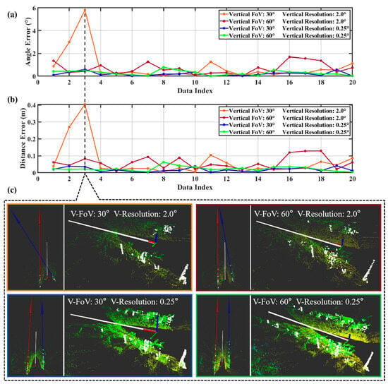
Figure 21.
Navigation-line-detection results under four different combinations of vertical FoV and vertical resolution. (a) Angular errors of the extracted navigation lines under four different combinations. (b) Distance errors of the extracted navigation lines under four different combinations. (c) Extracted navigation lines and tree trunk feature points under four different combinations.
In summary, when the system’s vertical FoV increases, it provides the system with a certain probability of extracting target point clouds from more data for navigation line detection. However, when the vertical FoV varies between 30° and 60°, the accuracy of navigation line detection is not sensitive to changes in vertical FoV. By contrast, the vertical resolution of the point cloud has a significant impact on the performance of navigation line detection, and it positively correlates with the accuracy of navigation line detection. High-resolution point clouds can provide more geometric information about tree rows, which facilitates the system in extracting more tree trunk feature points, thereby improving the accuracy of navigation line detection. Additionally, the experimental results also demonstrate that the rolling motion parameters selected in Section 2.2 of this study can ensure a relatively high perception performance.
3.2.4. Verification of System Generalization Across Various Orchard Structural Parameters
Since the 2D lidar rolling motion parameters (rolling angle, rolling speed) determining system performance in this study were obtained based on orchard scenes with fixed structural parameters, this study discusses the generalization of these parameters to orchards with different structural dimensions. The primary orchard structural parameters considered when selecting the rolling motion parameters were tree trunk height and tree row width. For tree trunk height, based on the results in Section 2.2, the selected parameters in this study ensure that the system can cover tree heights of up to 1 m above the ground, even with the minimum vertical scanning height range between rows. This indicates that in scenarios with different tree heights, when the tree trunk height is greater than that in the scenarios considered in this study, the system can at least obtain point clouds of the tree trunk up to 1 m in height. Conversely, when the tree trunk height is lower, the system’s vertical FoV can cover the entire trunk area of the tree. Additionally, the experimental results in Section 3.2.3 also prove that with a vertical FoV of 60°, variations in the point cloud height obtained by the system in the vertical direction have little impact on the navigation-line-detection results. Therefore, this system can adapt to most scenarios with varying tree trunk heights.
Regarding tree row width, its impact on system performance lies in the fact that when tree rows are too wide, due to the characteristic of 3D point clouds being denser nearby and sparser far away, the point clouds of the tree rows on both sides will become sparse, leading to the loss of geometric detail information in the vertical direction. According to the conclusions in Section 3.2.3, this can make it difficult for the system to extract sufficient tree trunk feature point clouds, ultimately affecting the accuracy of navigation line detection. Therefore, it is necessary to explore whether the system parameters selected in Section 2.2 are still applicable in scenarios with wide tree rows. To this end, this study modifies the Formulas (24) and (25) in Section 2.5.1 as follows:
Tree rows to the left of the current left tree row and the right of the current right tree row were extracted to simulate a working scenario with an average tree row width of 12 m (greater than the row width of most modern orchards). Subsequently, we used the same method described in Section 3.2.2 to extract and verify the accuracy of the navigation line, thereby validating the generalization of the system in orchard scenarios with wide tree rows. Figure 22a,b show the evaluation results of navigation-line-detection accuracy in the scenario with a 12 m row width. The average angular error is 0.205°, the average distance error is 0.026 m, the maximum angular error does not exceed 0.5°, and the maximum distance error does not exceed 0.05 m. These results are comparable to the navigation line accuracy obtained in the scenario with a 4 m row width, ensuring the perception accuracy for guidance between rows. Figure 22c shows the results of navigation line fitting and tree trunk feature point extraction. It can be seen that as the row spacing widens, the rolling 2D lidar is able to obtain more fruit tree point clouds in the vertical direction while also making the point clouds of the left and right tree rows become sparser. Nevertheless, a vertical resolution of 0.25° is sufficient to provide adequate geometric detail information, enabling the system to extract the main trunk point clouds of the fruit trees and use them to fit a high-accuracy navigation line.
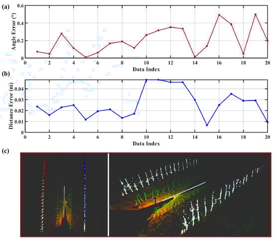
Figure 22.
Results of navigation line detection in a 12 m row width scenario. (a) Angular error of the navigation line. (b) Distance error of the navigation line. (c) Navigation line detection and tree trunk feature point extraction results.
In summary, the system designed in this study and the system parameters selected in Section 2.2 can ensure its generalization in most scenarios with different orchard structural parameters (tree height, row width).
4. Discussion
4.1. Discussion of Rolling 2D Lidar System Performance
The 3D point cloud acquired by the rolling 2D lidar in the modern orchard, as shown in Figure 15, demonstrates that the rolling motion parameters selected based on the structure of the orchard and the characteristics of the lidar effectively expand the system’s FoV and point cloud resolution. This allows for sufficient vertical FoV at any position between tree rows to encompass the 3D point cloud of the trunk area. Furthermore, the high point cloud resolution makes the structural features of the trunk area very distinct and clear. Figure 15 shows that even under the obstruction of dense lateral branches, some trunk point clouds can be visually distinguished, which lays the foundation for extracting trunk point clouds based on the local geometric features in Section 2.5.2.
The results in Figure 16 also demonstrate the effectiveness of the 3D point cloud motion distortion compensation method based on the combination of wheel odometry and IMU within a single scanning cycle. It can effectively restore the state of the 3D point cloud at a maximum moving speed of 0.5 m/s and under large-scale rotational movements. At the same time, this fused odometry information also provides the robot with motion state estimation within a single scanning cycle for robot control at a frequency of 50 Hz. The good results of point cloud motion compensation in Figure 16 also retroactively verify the effectiveness of the robot’s motion state estimation in a short period of time, providing a guarantee for robot motion control.
However, despite the promising performance demonstrated in the experiments, our system still requires further refinement and improvement in some aspects. The current motion state estimation method used in this study ignores the positioning errors caused by wheel slippage and sudden speed changes within a rolling cycle. Although the cumulative error of dead reckoning is generally small and negligible within a roll cycle in most cases, under specific circumstances such as the vehicle encountering a rock that causes a jump or navigating on excessively slippery grass that leads to significant wheel slippage, these aggressive changes in motion state can result in non-negligible positioning errors, thereby affecting the accuracy of the 3D point cloud in motion and causing its distortions. To address this issue, future study plans include incorporating 3D point cloud data into the implementation of lidar odometry and fusing them with wheel odometry and IMU data through the Kalman filter to form a LIWO (Lidar-Inertial-Wheel Odometry) system. This approach aims to eliminate the odometry drift caused by slippage, thereby enhancing the accuracy and robustness of motion state estimation and improving the quality of the 3D point cloud for autonomous navigation.
4.2. Discussion of 3D Point-Cloud-Based Navigation-Line-Detection Pipeline
The results in Figure 17 demonstrate the effectiveness of the point cloud filtering framework proposed in this study, particularly the use of odometry information and historical observations of tree row centerlines to predict the state of future tree row centerlines for the identification and extraction of left and right tree row point clouds. This method has been proven in experiments to successfully extract point cloud data for both left and right tree rows, even when the robot undergoes large-scale rotational movements within the rows. The results in Figure 19 further validate the effectiveness of trunk point cloud extraction based on geometric features and its importance for navigation line detection. Especially in summer, when fruit tree branches and leaves are very lush, accompanied by numerous lateral branches and foliage, as shown in Figure 23, the number and density of point clouds outside the tree trunks are often higher than those of the trunk point clouds. This can lead to the misidentification of canopy foliage point clouds as inliers when fitting tree row lines directly using RANSAC. Similarly, the method proposed by Nehme et al. [12,22,23], which involves calculating the point cloud histogram in the direction perpendicular to the tree rows to identify areas with higher point cloud density as more likely corresponding to the location of tree trunks, is no longer applicable in such environments. Areas with higher point cloud density tend to concentrate more in the lush lateral branch regions, causing the final fitted navigation line to deviate from the actual situation. However, the results in Figure 19 and Figure 20 show that by utilizing local geometric features and constraining the point cloud simultaneously in both the z-axis direction and the tree row distribution direction with RANSAC, the feature points in the trunk area can be better extracted, resulting in navigation lines with high accuracy (average distance errors of 0.023 m and 0.016 m, average angular errors of 0.272° and 0.146° at moving speeds of 0.2 m/s and 0.5 m/s, respectively).
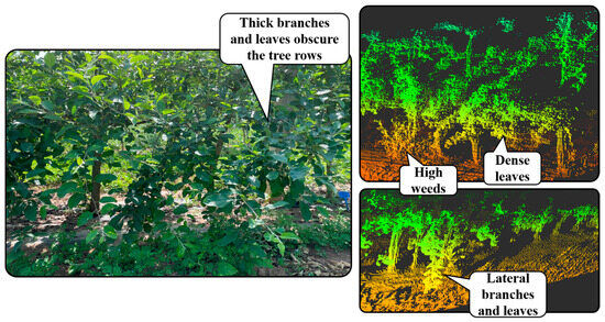
Figure 23.
The scene of dense lateral branches and leaves in summer.
Although current local point cloud features based on PCA are capable of extracting sufficient trunk candidate points to enable good performance in RANSAC tree row line fitting, in extreme scenarios with a small number of fruit tree trunks and severe occlusion, relying solely on PCA-based local point cloud features remains challenging for efficient trunk point cloud extraction. Therefore, future research intends to integrate texture and color information from images with 3D geometric information from point clouds and utilize the deep learning algorithm to achieve a semantic understanding of 3D environments. This will enable more robust obstacle recognition and localization, guiding robots to achieve more stable and fully autonomous operations in modern orchards.
5. Conclusions
In the semi-structured environment of modern orchards, accurately identifying and tracking tree rows has emerged as a crucial challenge for realizing perception-based autonomous navigation technology. Lidar, with its superior ranging accuracy and robust environmental interference resistance, is regarded as a promising sensor for advancing autonomous navigation in orchards. However, the commonly available 3D lidars on the market are limited by their narrow vertical FoV and sparse point cloud density, making it difficult to achieve precise recognition and positioning of fruit trees, in addition to their exorbitant cost. Additionally, autonomous navigation in orchards based on 3D point clouds often employs point cloud clustering or utilizes point cloud density distribution information to extract the tree row centerline for autonomous guidance. However, these methods are prone to deviations from actual conditions due to the influence of dense lateral branches, tree canopies, and weeds in the orchard. In response, this study introduces an innovative system based on rolling 2D lidar to acquire 3D point cloud data with high resolution and a large vertical FoV. Additionally, a pipeline for detecting navigation lines based on 3D point clouds is proposed, which utilizes predicted parameters of tree row centerlines to segment left and right tree rows. By combining PCA-based local geometric feature constraints with RANSAC, tree trunk feature points are extracted and used to fit the navigation centerline. Promising performance was achieved in outdoor experiments, with average distance errors of 0.023 m and 0.016 m, and average angular errors of 0.272° and 0.146° at moving speeds of 0.2 m/s and 0.5 m/s, respectively. This paves the way for an effective, economically efficient path for autonomous operations in modern orchards.
Furthermore, our future work will proceed in terms of two aspects. On the one hand, we aim to enhance the accuracy and robustness of system motion state estimation by integrating lidar-inertial odometry technology, thereby overcoming system localization errors caused by wheel slippage. On the other hand, we plan to leverage deep learning techniques to fuse image and point cloud features for a more enriched and stable understanding of 3D environments, guiding robots to achieve full automation in various orchard settings.
Author Contributions
Conceptualization, Y.Z. (Yibo Zhou); methodology, Y.Z. (Yibo Zhou), Y.Y. and X.W.; software, Y.Z. (Yibo Zhou); validation, Y.Z. (Yibo Zhou), X.W. and Z.W.; formal analysis, Y.Z. (Yibo Zhou); investigation, Y.Z. (Yibo Zhou), X.W. and Z.W.; resources, F.Z.; data curation, Y.Z. (Yibo Zhou); writing—original draft preparation, Y.Z. (Yibo Zhou); writing—review and editing, Y.Z. (Yanru Zhao); visualization, Y.Z. (Yibo Zhou); supervision, Y.Z. (Yanru Zhao) and K.Y.; project administration, Y.Z. (Yanru Zhao); funding acquisition, F.Z. All authors have read and agreed to the published version of the manuscript.
Funding
This research was funded by the Key Research and Development Project of Zhejiang Province, China (Program No.: 2023C02010).
Data Availability Statement
The data presented in this study are available upon request from the corresponding author.
Conflicts of Interest
The authors declare no conflicts of interest.
Abbreviations
The following abbreviations are used in this manuscript:
| AI | Artificial Intelligence |
| CZM | Concentric Zone Model |
| DOF | Degrees of Freedom |
| FoV | Field of View |
| GLE | Ground Likelihood Estimation |
| GNSS | Global Navigation Satellite System |
| IMU | Inertial Measurement Unit |
| IPC | Industrial Personal Computer |
| PCA | Principal Component Analysis |
| RANSAC | Random Sample Consensus |
| R-GPF | Region-wise Ground Plane Fitting |
| RTK | Real-Time Kinematic |
| SLERP | Spherical Linear Interpolation |
References
- Xie, B.; Jin, Y.; Faheem, M.; Gao, W.; Liu, J.; Jiang, H.; Cai, L.; Li, Y. Research progress of autonomous navigation technology for multi-agricultural scenes. Comput. Electron. Agric. 2023, 211, 107963. [Google Scholar] [CrossRef]
- Zhou, H.Y.; Wang, X.; Au, W.; Kang, H.W.; Chen, C. Intelligent robots for fruit harvesting: Recent developments and future challenges. Precis. Agric. 2022, 23, 1856–1907. [Google Scholar] [CrossRef]
- Durand-Petiteville, A.; Le Flécher, E.; Cadenat, V.; Sentenac, T.; Vougioukas, S. Tree detection with low-cost 3D sensors for autonomous navigation in orchards. IEEE Robot. Autom. Lett. 2018, 3, 3876–3883. [Google Scholar] [CrossRef]
- Shi, J.; Bai, Y.; Diao, Z.; Zhou, J.; Yao, X.; Zhang, B. Row Detection BASED Navigation and Guidance for Agricultural Robots and Autonomous Vehicles in Row-Crop Fields: Methods and Applications. Agronomy 2023, 13, 1780. [Google Scholar] [CrossRef]
- Elsheikh, M.; Iqbal, U.; Noureldin, A.; Korenberg, M. The Implementation of Precise Point Positioning (PPP): A Comprehensive Review. Sensors 2023, 23, 8874. [Google Scholar] [CrossRef]
- Jiang, S.; Qi, P.; Han, L.; Liu, L.; Li, Y.; Huang, Z.; Liu, Y.; He, X. Navigation system for orchard spraying robot based on 3D LiDAR SLAM with NDT_ICP point cloud registration. Comput. Electron. Agric. 2024, 220, 108870. [Google Scholar] [CrossRef]
- Wang, T.; Chen, B.; Zhang, Z.; Li, H.; Zhang, M. Applications of machine vision in agricultural robot navigation: A review. Comput. Electron. Agric. 2022, 198, 107085. [Google Scholar] [CrossRef]
- Xu, S.; Rai, R. Vision-based autonomous navigation stack for tractors operating in peach orchards. Comput. Electron. Agric. 2024, 217, 108558. [Google Scholar] [CrossRef]
- Liu, S.; Wang, X.; Li, S.; Chen, X.; Zhang, X. Obstacle avoidance for orchard vehicle trinocular vision system based on coupling of geometric constraint and virtual force field method. Expert Syst. Appl. 2022, 190, 116216. [Google Scholar] [CrossRef]
- Fei, Z.; Vougioukas, S. Row-sensing templates: A generic 3D sensor-based approach to robot localization with respect to orchard row centerlines. J. Field Robot. 2022, 39, 712–738. [Google Scholar] [CrossRef]
- Zhou, J.; Geng, S.; Qiu, Q.; Shao, Y.; Zhang, M. A Deep-Learning Extraction Method for Orchard Visual Navigation Lines. Agriculture 2022, 12, 1650. [Google Scholar] [CrossRef]
- Higuti, V.A.H.; Velasquez, A.E.B.; Magalhaes, D.V.; Becker, M.; Chowdhary, G. Under canopy light detection and ranging-based autonomous navigation. J. Field Robot. 2019, 36, 547–567. [Google Scholar] [CrossRef]
- Malavazi, F.B.P.; Guyonneau, R.; Fasquel, J.-B.; Lagrange, S.; Mercier, F. LiDAR-only based navigation algorithm for an autonomous agricultural robot. Comput. Electron. Agric. 2018, 154, 71–79. [Google Scholar] [CrossRef]
- Blok, P.M.; van Boheemen, K.; van Evert, F.K.; Ijsselmuiden, J.; Kim, G.-H. Robot navigation in orchards with localization based on Particle filter and Kalman filter. Comput. Electron. Agric. 2019, 157, 261–269. [Google Scholar] [CrossRef]
- Iberraken, D.; Gaurier, F.; Roux, J.-C.; Chaballier, C.; Lenain, R. Autonomous Vineyard Tracking Using a Four-Wheel-Steering Mobile Robot and a 2D LiDAR. AgriEngineering 2022, 4, 826–846. [Google Scholar] [CrossRef]
- Jiang, A.; Ahamed, T. Navigation of an Autonomous Spraying Robot for Orchard Operations Using LiDAR for Tree Trunk Detection. Sensors 2023, 23, 4808. [Google Scholar] [CrossRef]
- Xia, Y.; Lei, X.; Pan, J.; Chen, L.; Zhang, Z.; Lyu, X. Research on orchard navigation method based on fusion of 3D SLAM and point cloud positioning. Front. Plant Sci. 2023, 14, 1207742. [Google Scholar] [CrossRef]
- Wang, S.; Song, J.; Qi, P.; Yuan, C.; Wu, H.; Zhang, L.; Liu, W.; Liu, Y.; He, X. Design and development of orchard autonomous navigation spray system. Front. Plant Sci. 2022, 13, 960686. [Google Scholar] [CrossRef]
- Liu, W.; Li, W.; Feng, H.; Xu, J.; Yang, S.; Zheng, Y.; Liu, X.; Wang, Z.; Yi, X.; He, Y.; et al. Overall integrated navigation based on satellite and lidar in the standardized tall spindle apple orchards. Comput. Electron. Agric. 2024, 216, 108489. [Google Scholar] [CrossRef]
- Liu, L.; Liu, Y.; He, X.; Liu, W. Precision Variable-Rate Spraying Robot by Using Single 3D LIDAR in Orchards. Agronomy 2022, 12, 2509. [Google Scholar] [CrossRef]
- Velodyne. VLP-16 in VLP-16 Manual: User’s Manual and Programming Guide; Velodyne LiDAR: San Jose, CA, USA, 2016. [Google Scholar]
- Nehme, H.; Aubry, C.; Solatges, T.; Savatier, X.; Rossi, R.; Boutteau, R. LiDAR-based Structure Tracking for Agricultural Robots: Application to Autonomous Navigation in Vineyards. J. Intell. Robot. Syst. 2021, 103, 16. [Google Scholar] [CrossRef]
- Zhang, J.; Chambers, A.; Maeta, S.; Bergerman, M.; Singh, S. 3D perception for accurate row following: Methodology and results. In Proceedings of the IEEE/RSJ International Conference on Intelligent Robots & Systems, Tokyo, Japan, 3–7 November 2013. [Google Scholar]
- Crocetti, F.; Bellocchio, E.; Dionigi, A.; Felicioni, S.; Costante, G.; Fravolini, M.L.; Valigi, P. ARD-VO: Agricultural robot data set of vineyards and olive groves. J. Field Robot. 2023, 40, 1678–1696. [Google Scholar] [CrossRef]
- Huang, C.; Cai, D.; Wang, W.; Li, J.; Duan, J.; Yang, Z. Development of an automatic control system for a hydraulic pruning robot. Comput. Electron. Agric. 2023, 214, 108329. [Google Scholar] [CrossRef]
- Xu, R.; Li, C. A modular agricultural robotic system (MARS) for precision farming: Concept and implementation. J. Field Robot. 2022, 39, 387–409. [Google Scholar] [CrossRef]
- Gai, J.; Xiang, L.; Tang, L. Using a depth camera for crop row detection and mapping for under-canopy navigation of agricultural robotic vehicle. Comput. Electron. Agric. 2021, 188, 106301. [Google Scholar] [CrossRef]
- Alismail, H.; Browning, B. Automatic Calibration of Spinning Actuated Lidar Internal Parameters. J. Field Robot. 2015, 32, 723–747. [Google Scholar] [CrossRef]
- Lim, H.; Oh, M.; Myung, H. Patchwork: Concentric Zone-Based Region-Wise Ground Segmentation with Ground Likelihood Estimation Using a 3D LiDAR Sensor. IEEE Robot. Autom. Lett. 2021, 6, 6458–6465. [Google Scholar] [CrossRef]
- LSLiDAR. C16 User’s Manual; LSLiDAR: Shenzhen, China, 2024. [Google Scholar]
- LSLiDAR. C32 User’s Manual; LSLiDAR: Shenzhen, China, 2024. [Google Scholar]
- Ouster. Mid-Range High-Resolution Imaging Lidar OS1; Ouster: San Francisco, CA, USA, 2025. [Google Scholar]
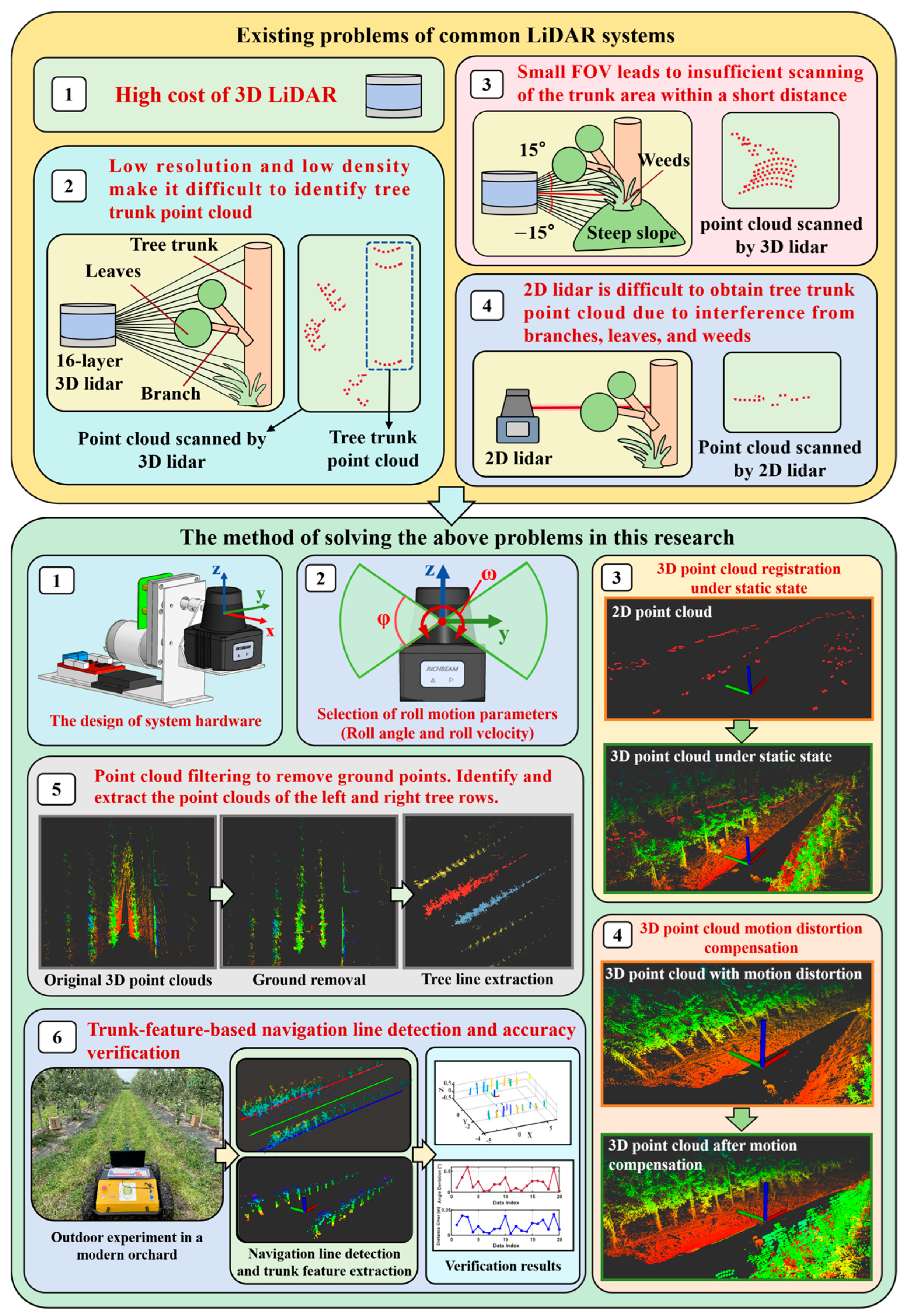
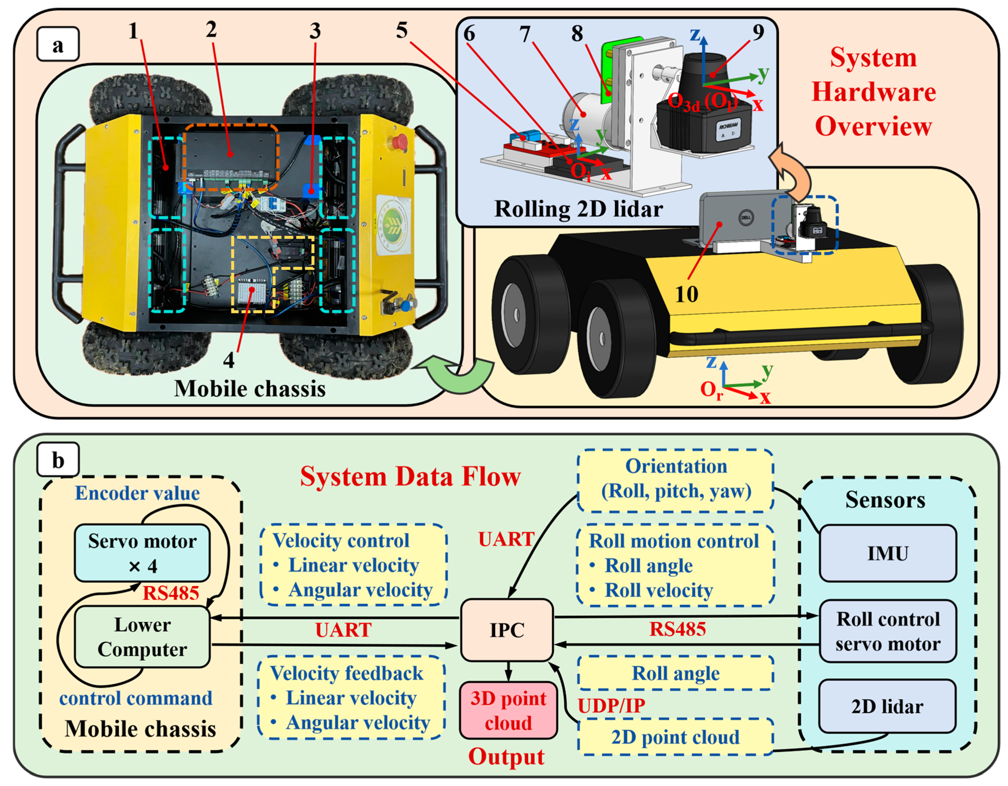
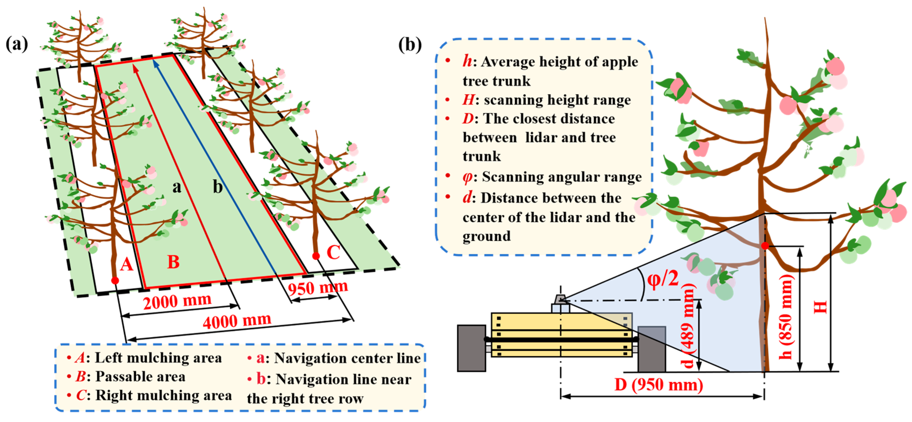
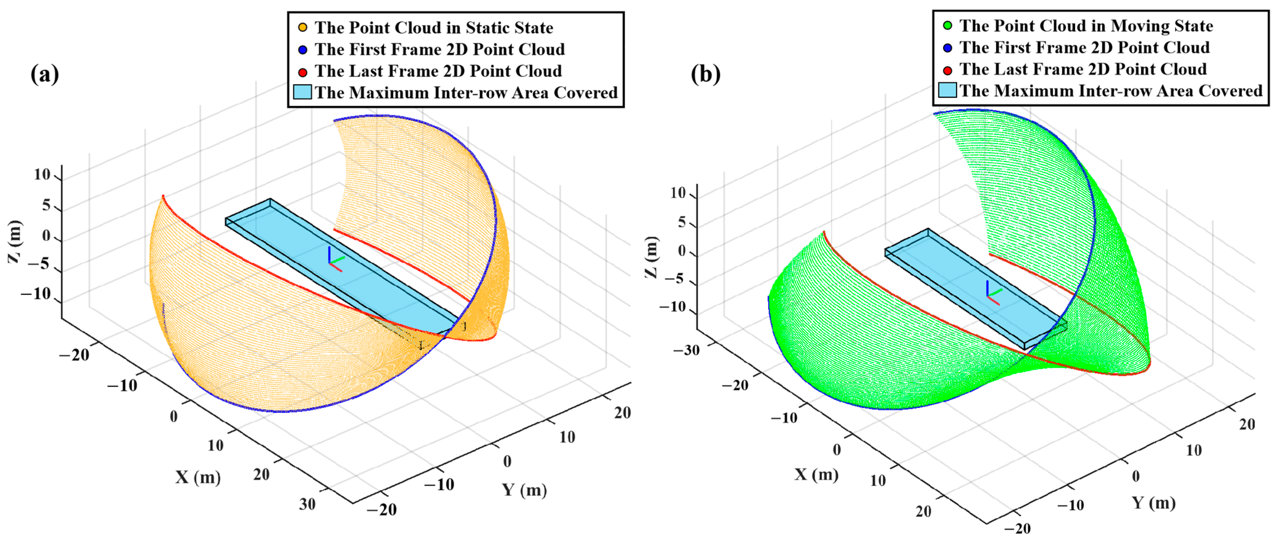
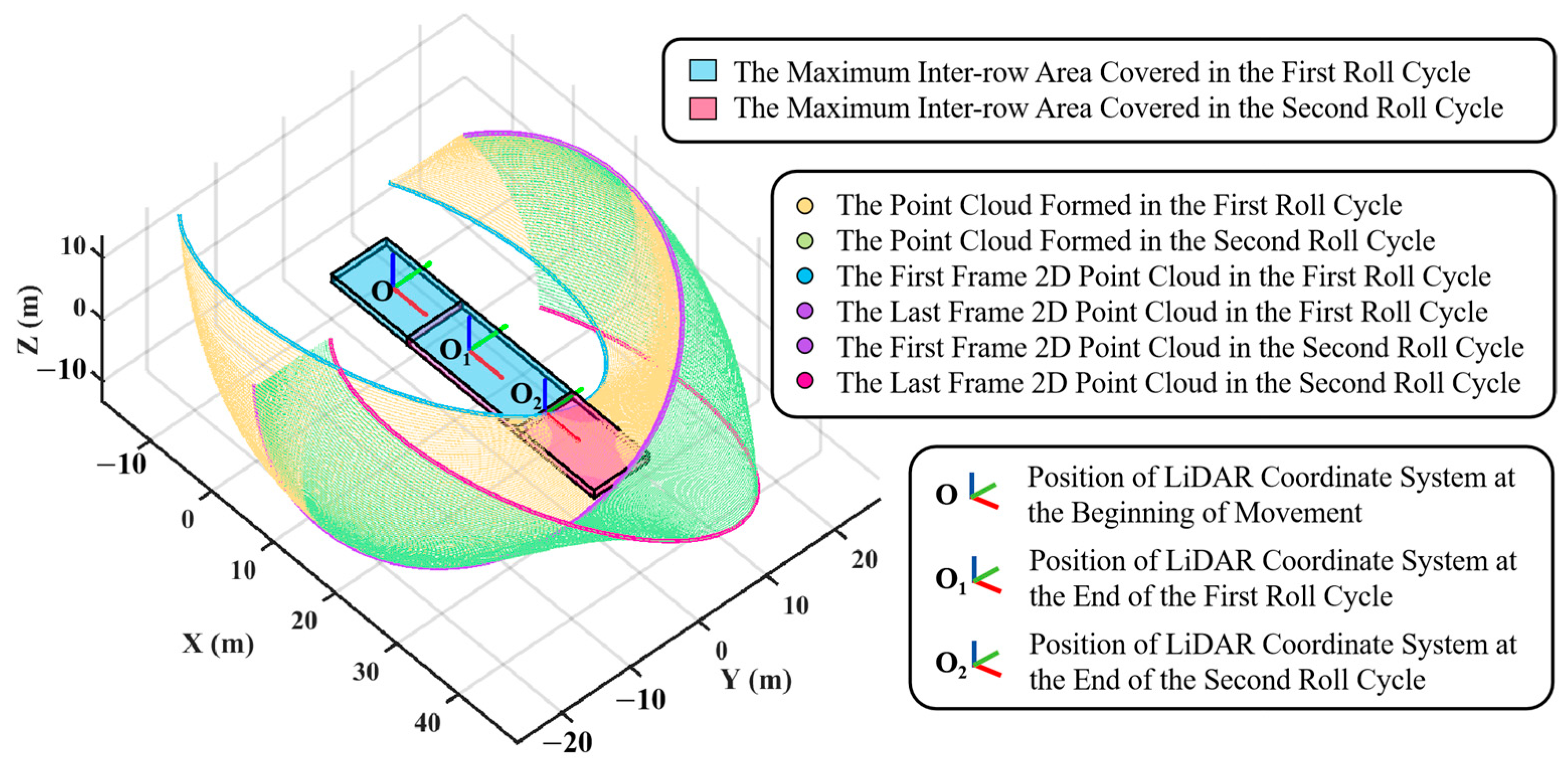
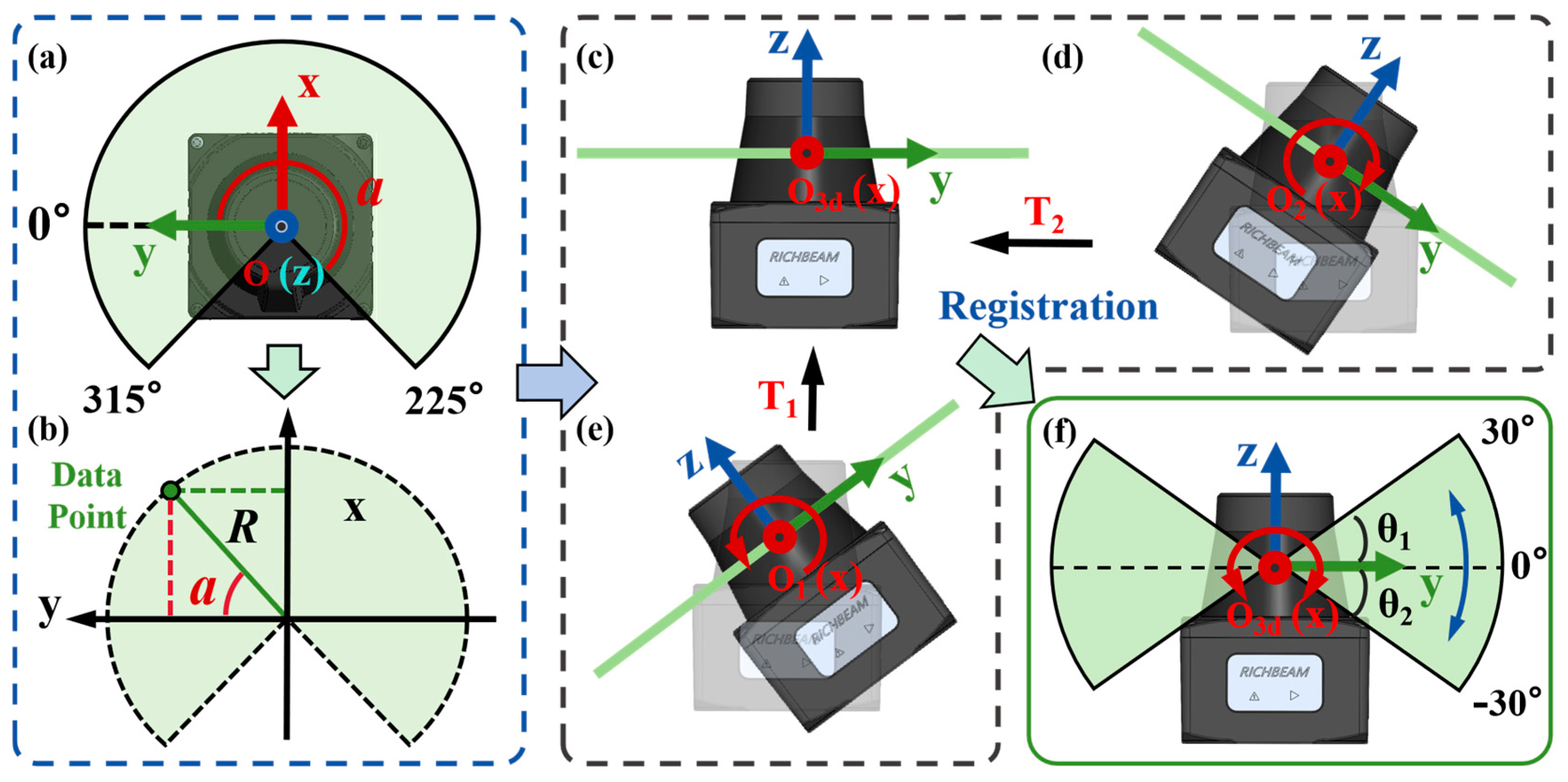
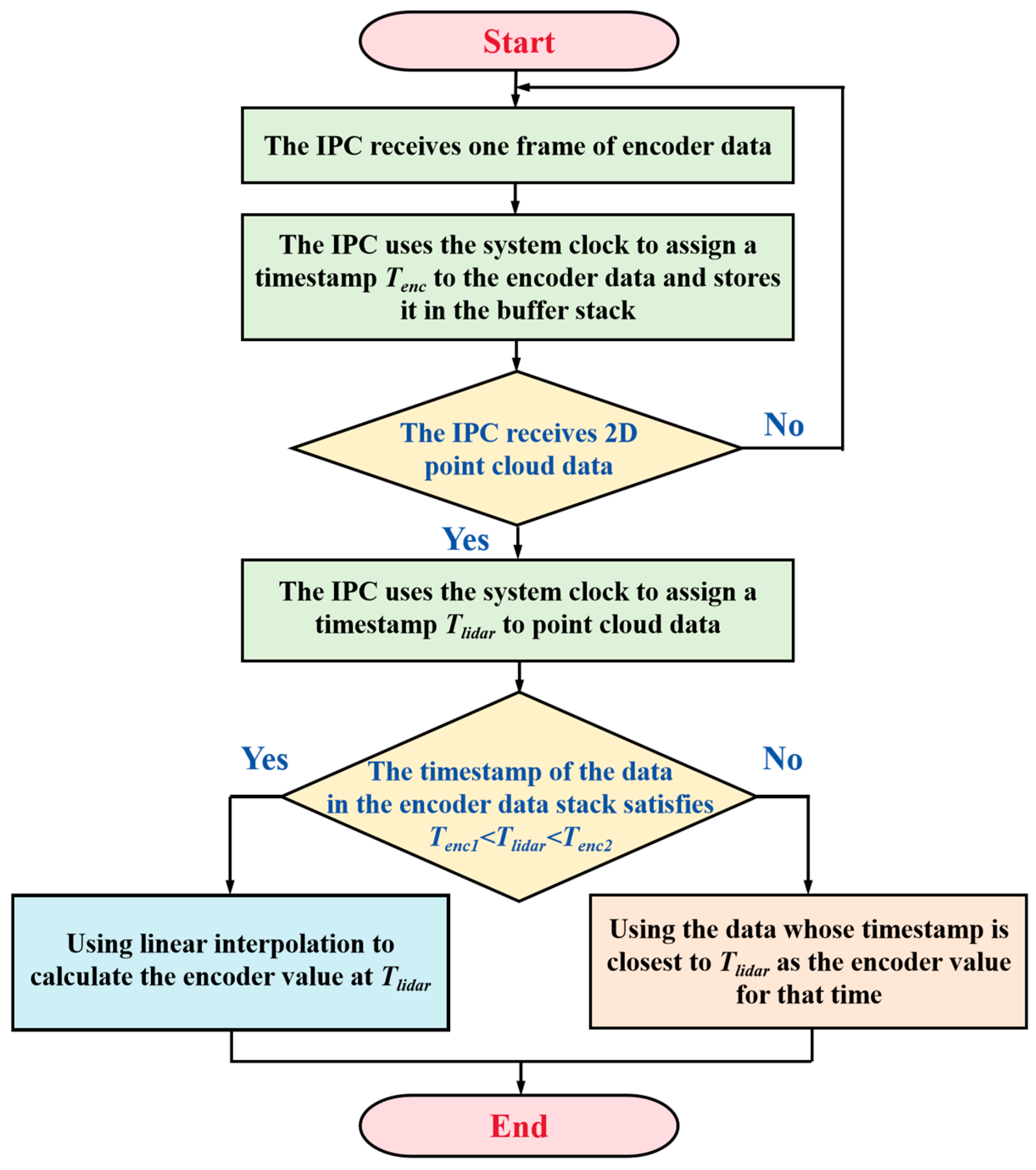
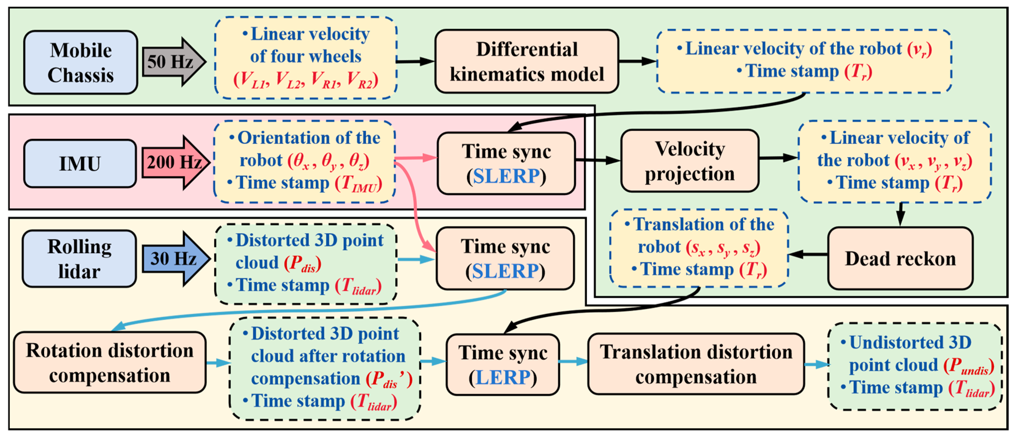
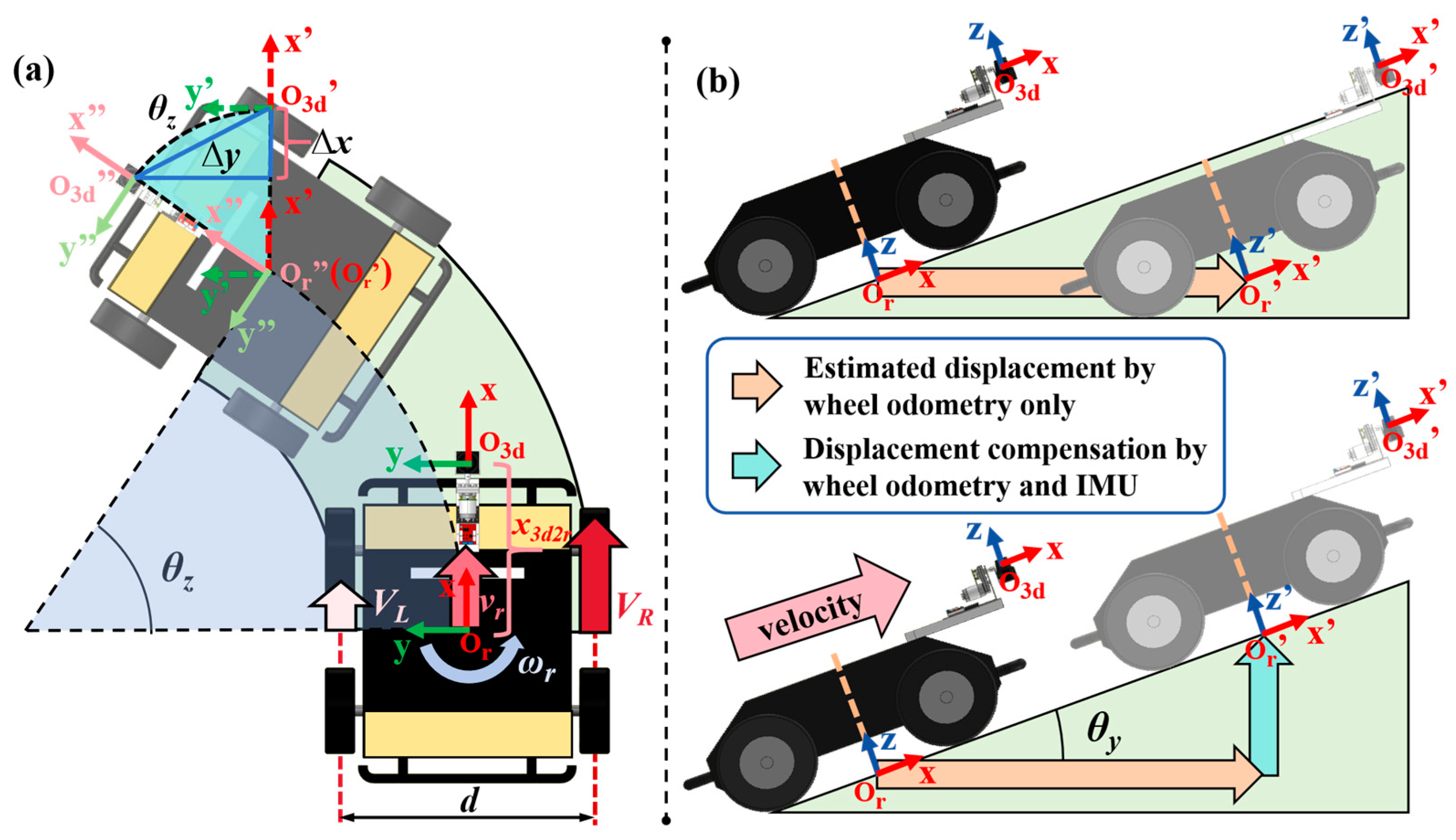
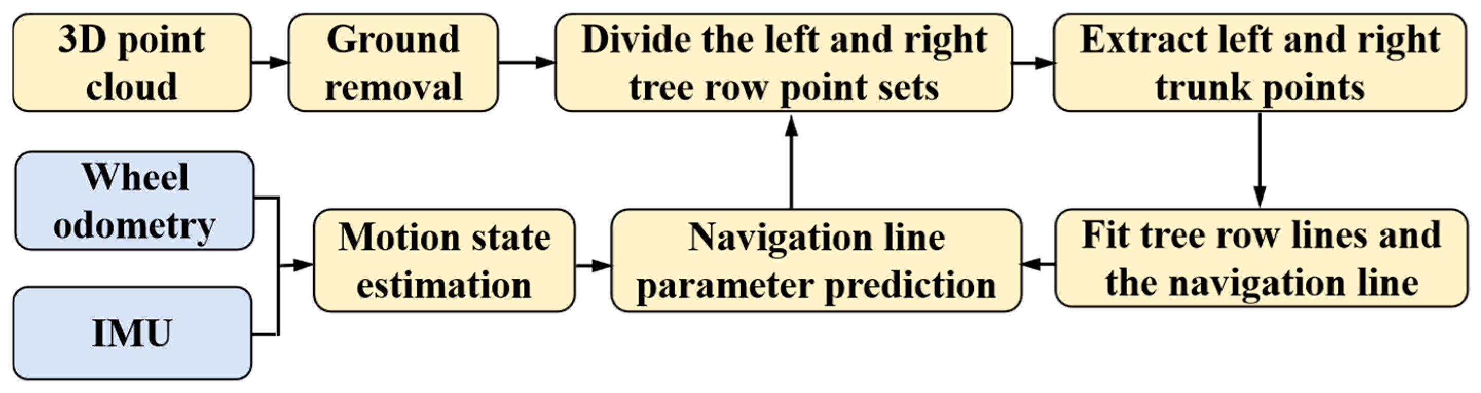


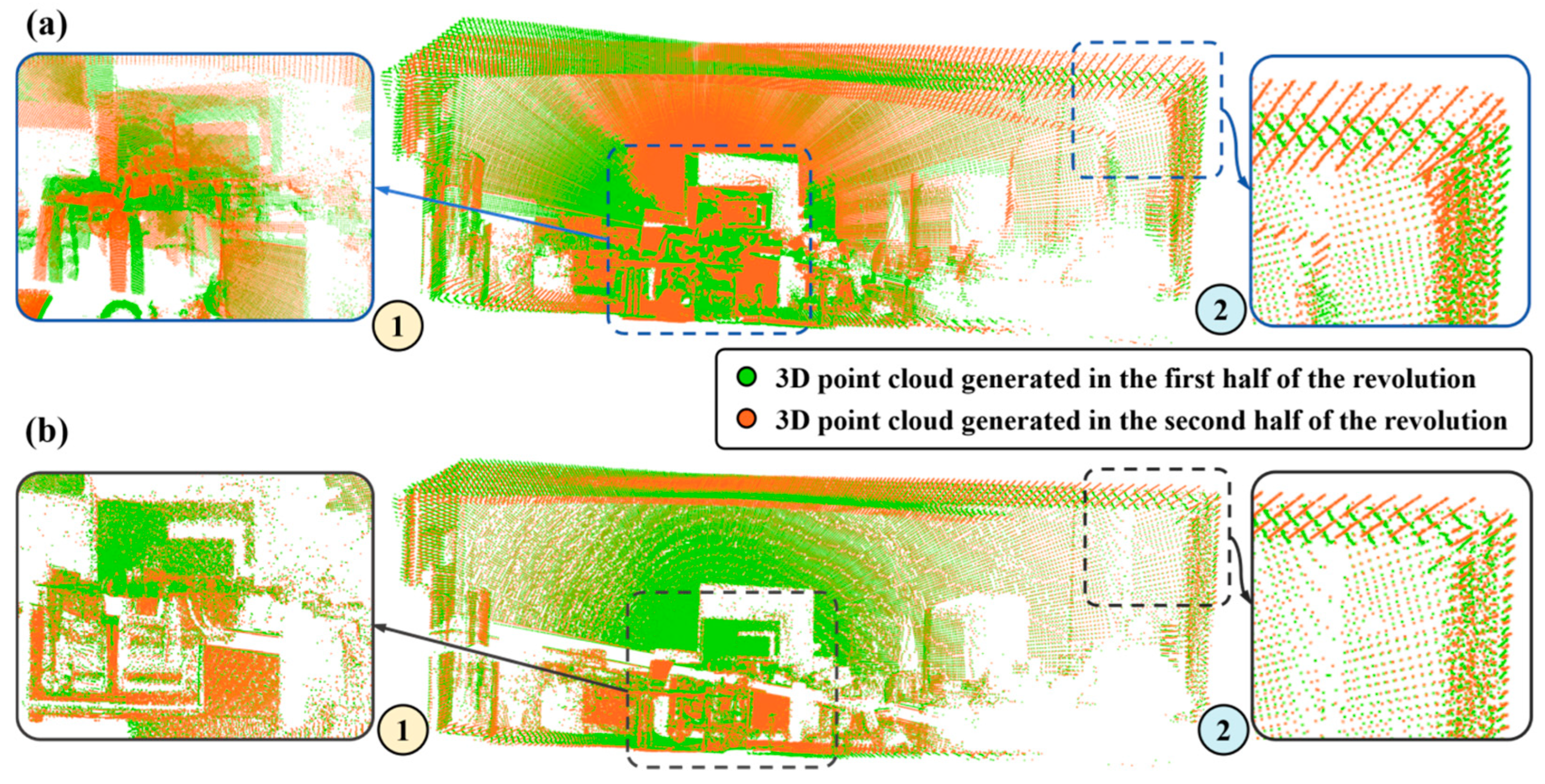
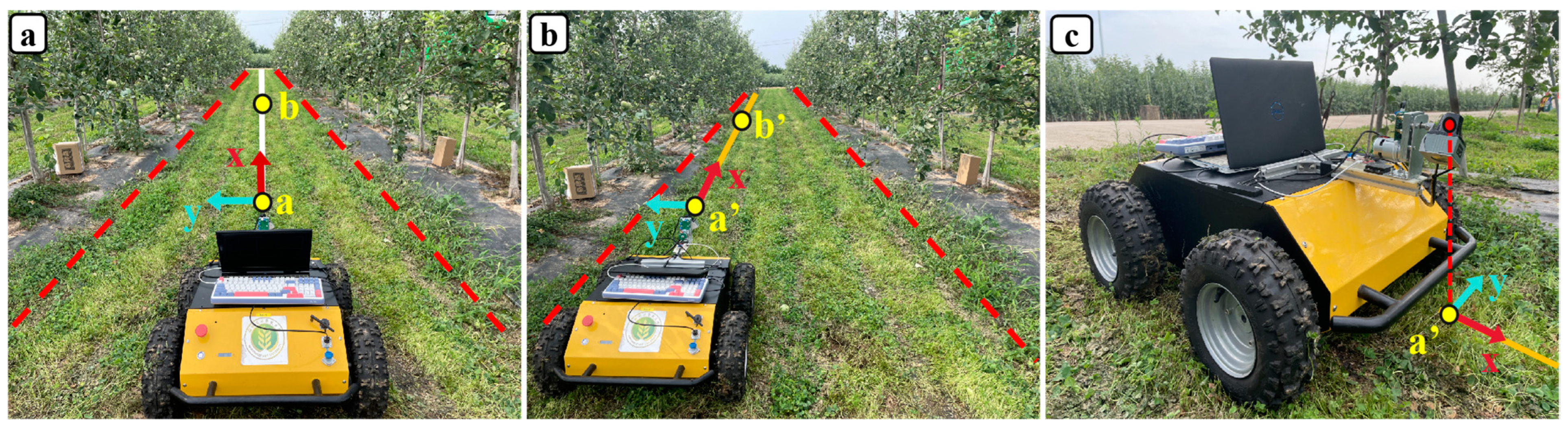
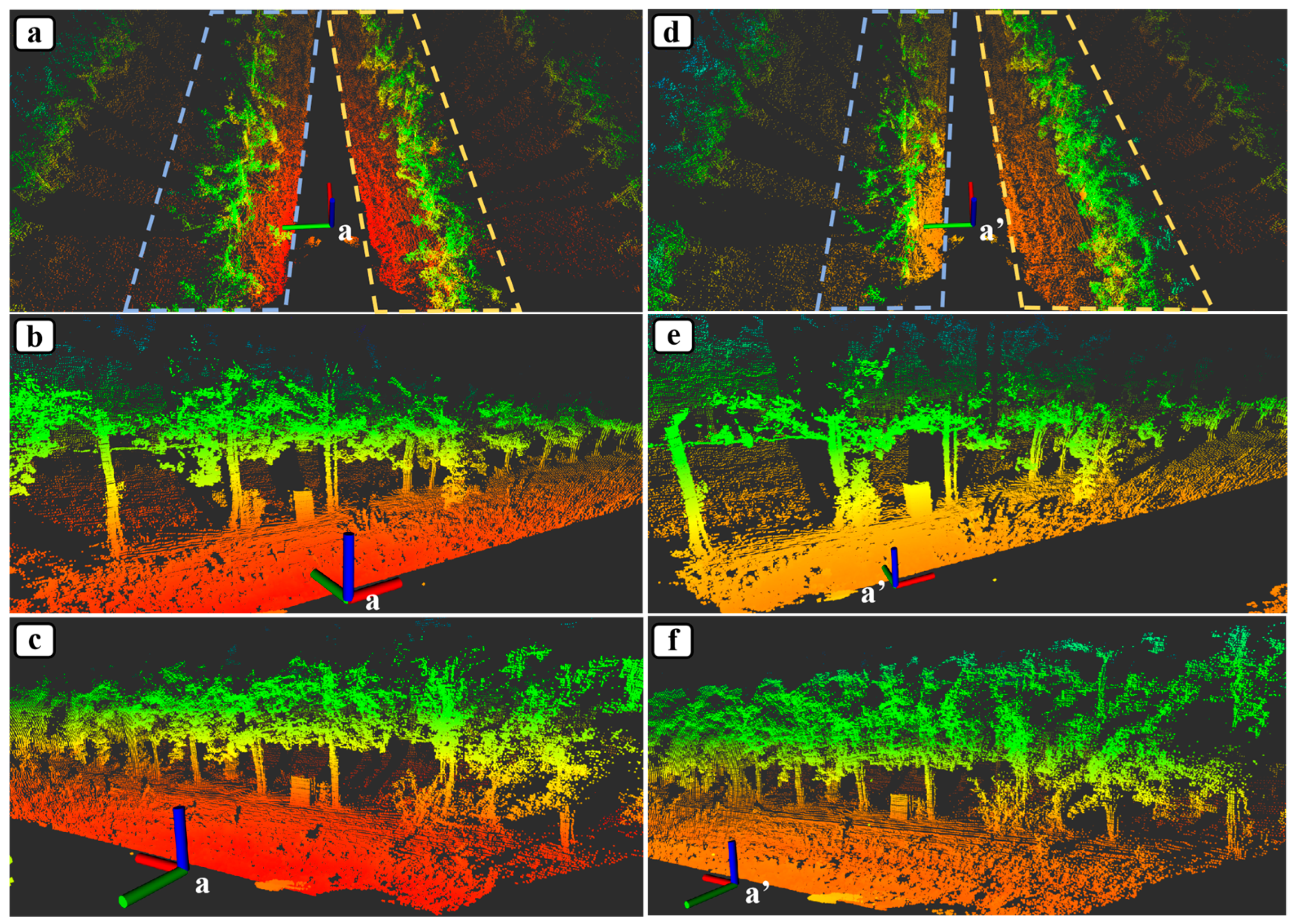
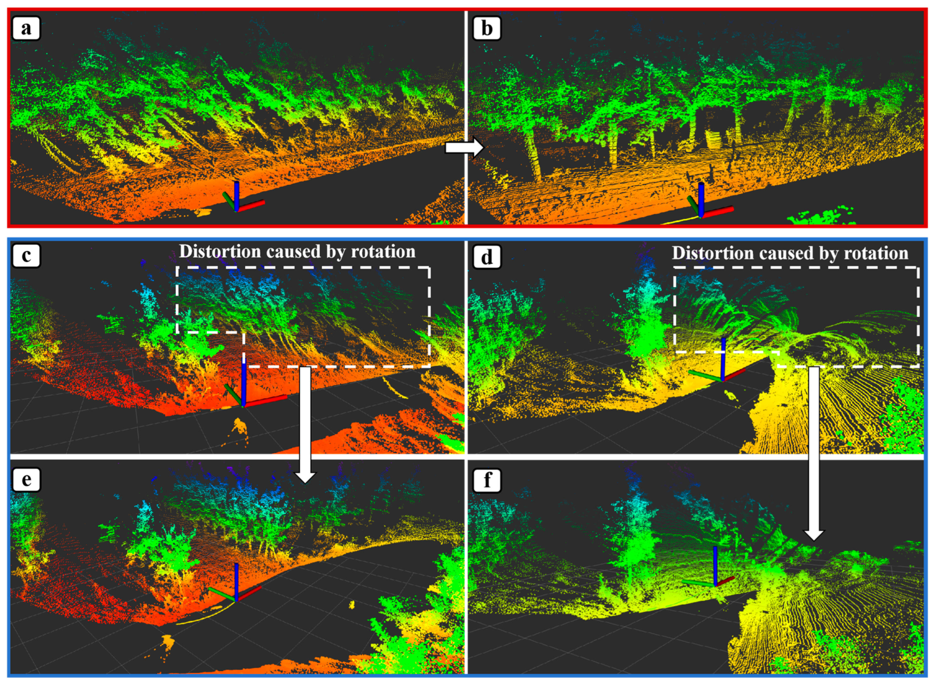

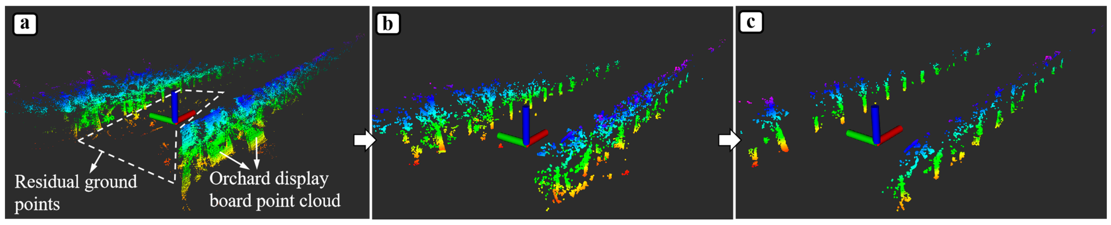

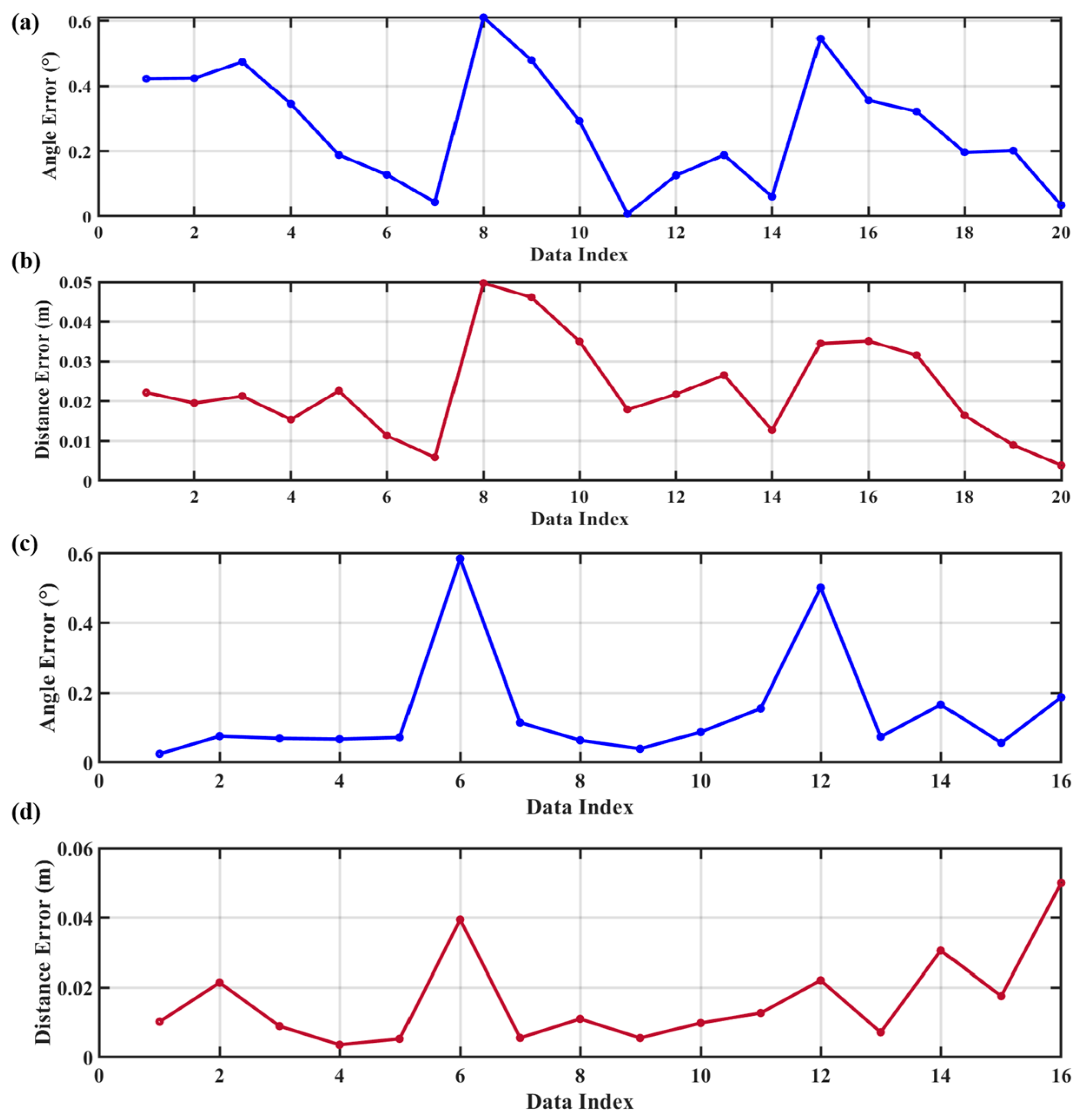
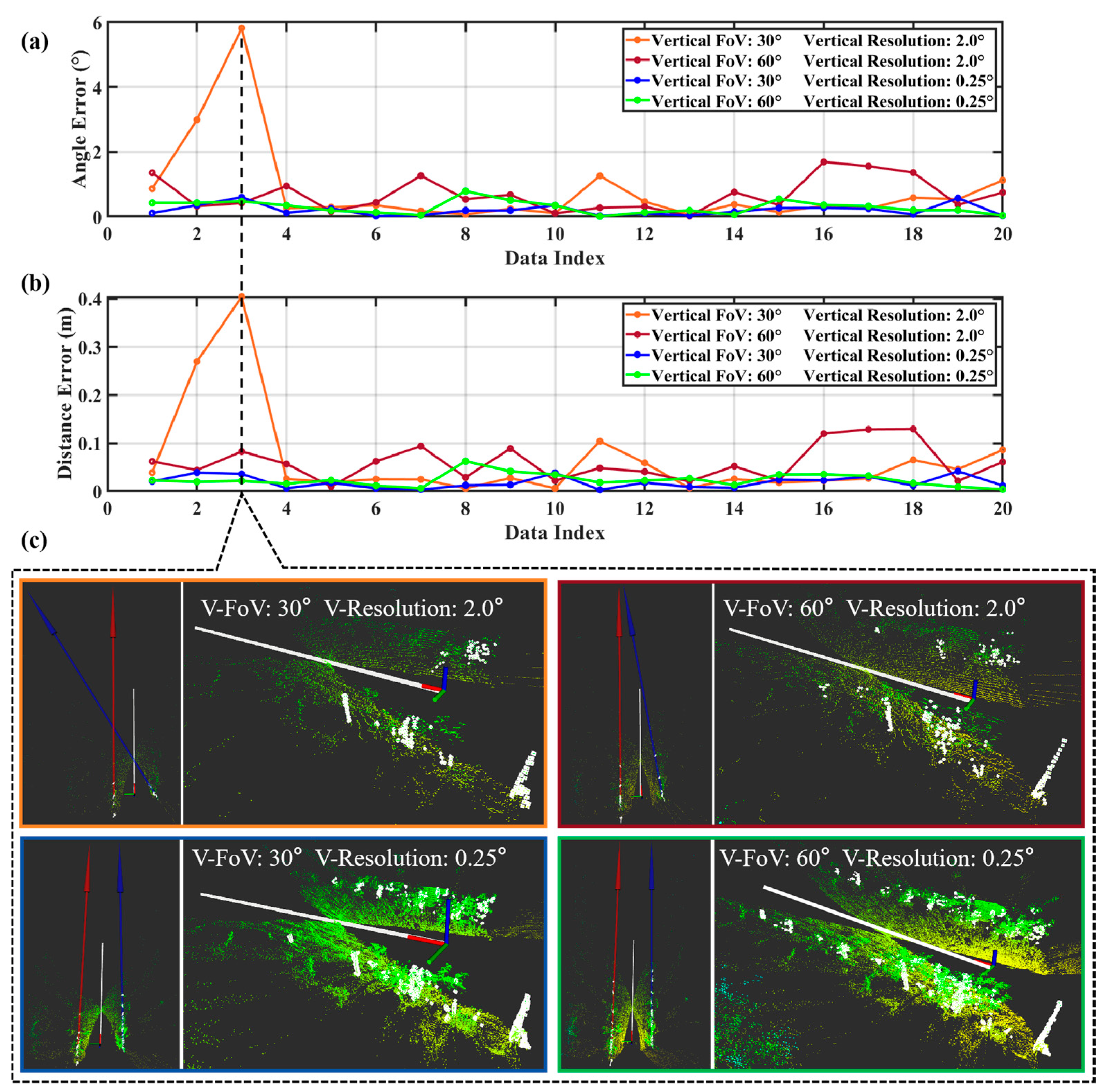
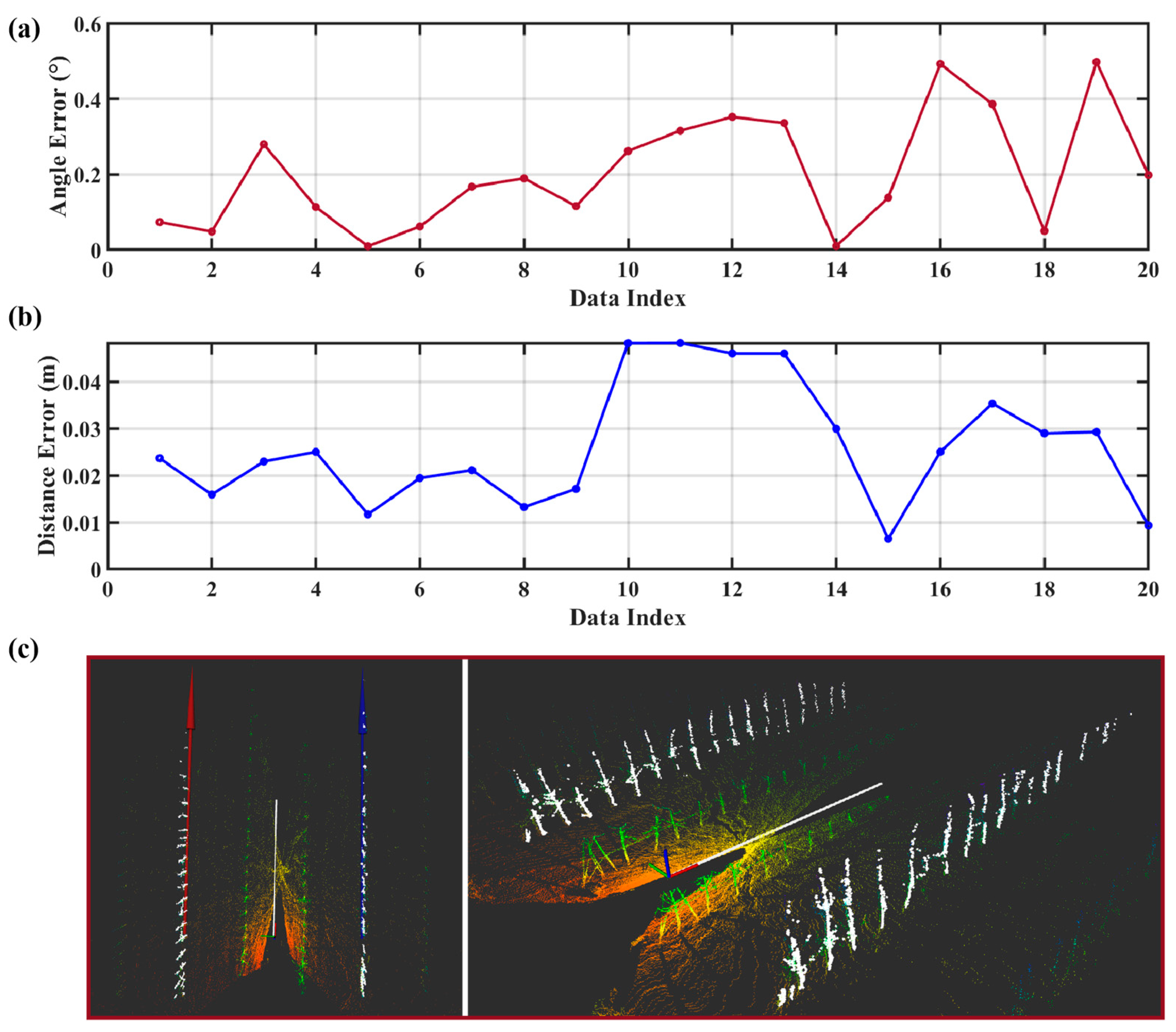
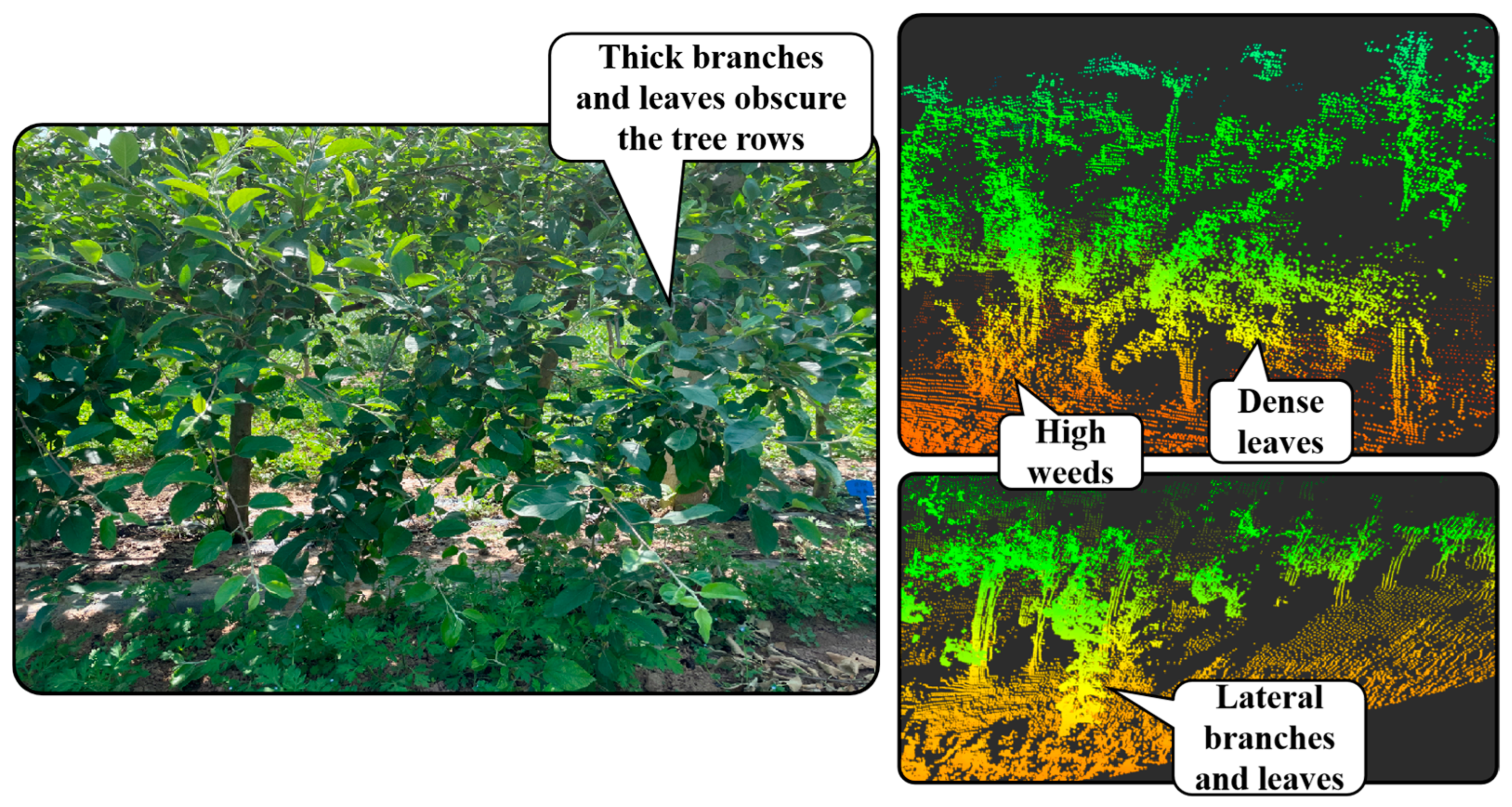
Disclaimer/Publisher’s Note: The statements, opinions and data contained in all publications are solely those of the individual author(s) and contributor(s) and not of MDPI and/or the editor(s). MDPI and/or the editor(s) disclaim responsibility for any injury to people or property resulting from any ideas, methods, instructions or products referred to in the content. |
© 2025 by the authors. Licensee MDPI, Basel, Switzerland. This article is an open access article distributed under the terms and conditions of the Creative Commons Attribution (CC BY) license (https://creativecommons.org/licenses/by/4.0/).