Article

Combined Mechanical–Chemical Weed Control Methods in Post-Emergence Strategy Result in High Weed Control Efficacy in Sugar Beet

by
Jakob Berg
1,*,
Helmut Ring
2 and
Heinz Bernhardt
1
1
Agricultural Systems Engineering, Technical University of Munich, Dürnast 10, 85354 Freising, Germany
2
Verband Bayerischer Zuckerrübenanbauer e.V., Sandstraße 4, 93092 Barbing, Germany
*
Author to whom correspondence should be addressed.
Agronomy 2025, 15(4), 879; https://doi.org/10.3390/agronomy15040879
Submission received: 11 March 2025 / Revised: 27 March 2025 / Accepted: 29 March 2025 / Published: 31 March 2025
(This article belongs to the Section Weed Science and Weed Management)

Abstract

:
Against the backdrop of increasing herbicide resistance and societal and political objectives for reducing plant protection products, combinations of mechanical and herbicide weed control methods are gaining importance. In row crops such as sugar beet, the use of mechanical hoeing between crop rows (interrow) combined with band spraying of herbicides within rows (intrarow) can lead to significant herbicide savings compared to standard broadcast herbicide applications. However, effective weed control remains crucial. In this study, a two-year field experiment was conducted to evaluate different combinations of band spraying, mechanical hoeing, and broadcast spraying in post-emergence weed control applications in sugar beet. The weed control efficacy of each treatment was assessed relative to an untreated control using weed counting to determine absolute weed density and image analysis to quantify weed cover. Compared to the untreated control, total weed control efficiencies of up to 90.8% (weed counting) and 99.5% (image analysis) were achieved. In comparison to three consecutive broadcast herbicide applications, the mechanical–chemical combinations resulted in a similar or even superior weed control efficacy while enabling herbicide reductions of up to 65.59%. These results highlight the valuable potential of mechanical–chemical weed control combinations for herbicide-reduced weed management within post-emergence application systems in sugar beet. They represent a key tool in the context of integrated weed management (IWM).

1. Introduction

Sugar beet (Beta vulgaris L.) constitutes approximately 20% of global sugar production, ranking second among sugar crops after sugarcane [1]. In addition to fertile site conditions with deep soils and a temperate climate [2], successful sugar beet cultivation requires intensive crop protection. Weed control plays a particularly crucial role during the early growth stages of sugar beet when the crop is still weakly competitive [3,4]. The slow juvenile development of sugar beet [5,6] and the row-based cultivation system with wide row spacing result in delayed canopy closure, favoring the establishment of early- and fast-growing weed species [7,8]. Sugar beet competes intensely with weeds for sunlight [6], water, and nutrients [9,10]. If weed control is omitted or insufficient, substantial yield losses can occur [11,12,13]. Thus, effective weed control is essential for high-yielding sugar beet production.
Under European growing conditions, weed control in sugar beet cultivation has primarily relied on broadcast applications of herbicides post-emergence [6,14,15]. Roßberg et al. [16] report an average herbicide application frequency of 3.5–3.9 in German sugar beet production. Commonly applied active ingredients include metamitron, phenmedipham, and ethofumesate [17,18]. However, the increasing development of herbicide-resistant weed populations [10,18] and the resulting loss of sensitivity to established sugar beet herbicides pose significant challenges. Chenopodium album is considered a key weed species in sugar beet cultivation [5,19] and has shown increasing resistance to metamitron in recent years [18,19,20]. Similarly, resistant biotypes of Amaranthus retroflexus against metamitron have been reported [18]. Another critical issue is that no new modes of action have been introduced for decades [18,21]. It is evident that well-planned herbicide weed control remains crucial in sugar beet cultivation to maintain the efficacy of the remaining available herbicides. Zwerger et al. [22] emphasize that each herbicide application exerts additional selection pressure. Consequently, relying exclusively on herbicide weed control in sugar beet production is becoming increasingly challenging. Therefore, an integrated weed management (IWM) system is more important than ever.
A promising approach for reducing herbicide use in sugar beet cultivation—thus mitigating selection pressure—is the implementation of mechanical weed control and combined mechanical–chemical weed management strategies [23,24,25]. The row-based cultivation system of sugar beet allows for targeted weed control: emerging weeds between the rows (interrow) can be mechanically removed using a hoe, while weeds within the rows (intrarow) can be chemically controlled using a band sprayer. The use of modern, camera-guided hoeing systems and band sprayers has gained increasing relevance in standard sugar beet farming in recent years due to the need to prevent herbicide resistance and to meet societal and political pesticide reduction targets [26,27].
To evaluate the efficacy of different combinations of mechanical and herbicidal weed control methods in terms of sufficient weed control and simultaneous herbicide savings within an integrated weed management approach, a two-year field experiment was conducted in 2023 and 2024 in an intensive sugar-beet-growing region in Lower Bavaria, southeastern Germany. In the context of a standard three-pass post-emergence application (post-em.) system, three methods were combined: broadcast herbicide application, combinations of herbicide band spraying in the intrarow and interrow hoeing, and interrow hoeing without herbicides. To assess the weed control efficacy of each treatment, both weed counting for determining weed density and image analysis for quantifying weed cover were conducted after the third post-emergence application. The following hypothesis should be tested: The use of mechanical–chemical combinations for weed control in three post-emergence applications in sugar beet results in similar weed control efficacy compared to solo broadcast herbicide spraying.

2. Materials and Methods

2.1. Sites and Weather Conditions

For the two-year experimental trial, two agricultural fields were selected that were in close proximity to each other and continuously subjected to intensive practical land cultivation under the same crop rotation (sugar beet, starch potato, winter wheat). The fields were located near Innerhienthal in the Gäuboden region of Lower Bavaria, southeastern Germany, close to Straubing (Field 2023: 48°50′44.38″ N, 12°34′51.96″ E, 341 m altitude; Field 2024: 48°50′41.60″ N, 12°35′02.22″ E, 341 m altitude). The exact soil type of the experimental site is classified as haplic luvisol (WRB) [28] on loess.
Table 1 presents the monthly weather data for the months of March to October at the experimental site, including the long-term average (2012–2022) as well as the conditions observed in the two experimental years, 2023 and 2024.

2.2. Crop Management

In both years, the variety BTS 2045 was sown. The preceding crop on the experimental fields was winter wheat, followed by a catch crop. The catch crop consisted of white mustard (Sinapis alba) and was grown for the purpose of reducing nutrient leaching, particularly nitrate. It was sown on 26 August 2022 and on 19 August 2023, respectively. The mulching process was carried out on 15 November in each year. Subsequently, the fields were plowed to 35 cm on 17 November 2022 and on 18 November 2023, respectively. Nitrogen fertilization was based on the results of soil sample analyses using the EUF method (electro-ultrafiltration). Fertilization was carried out the day before seedbed preparation. In 2023, 130 kg N/ha and in 2024, 135 kg N/ha were broadcast in the form of granulated calcium ammonium nitrate. After shallow seedbed preparation with a rotary harrow, which was conducted the day before sugar beet sowing and created a fine and consolidated seedbed, sugar beet sowing was performed on 21 March 2023, in the first trial year, and on 28 March 2024, in the second year. The seeds were sown at 3 cm deep, standard row spacing of 50 cm, and an intrarow seed spacing of 18 cm. Insecticidal plant protection measures against flea beetles and fungicidal treatments, primarily targeting Cercospora beticola, were applied in both years after the corresponding damage thresholds were reached.

2.3. Experimental Design

The two-year field experiment was conducted using a randomized complete block design with four replications. A total of 60 plots, each measuring 6 m in width and 16 m in length (96 m2), were established in each year. There were fifteen treatments, including an untreated control without weed control as well as combining different weed control methods: “broadcast herbicide application” (broadcast: br), “mechanical hoeing” (hoe: h), and a combination of “herbicide band application” and “mechanical hoeing” (band/hoe: b/h). Table 2 provides a detailed overview of the individual experimental treatments and their respective herbicide reduction potential compared to the solo broadcast herbicide application treatment (treatment 9). The herbicide savings potential was calculated cumulatively for all three post-em. based on the amount of applicated herbicides applied per hectare.
A 5 m buffer zone between each block replication provided space for acceleration and deceleration during machine operations. This ensured consistent working speeds for the hoeing and spraying treatments within the assessment areas.

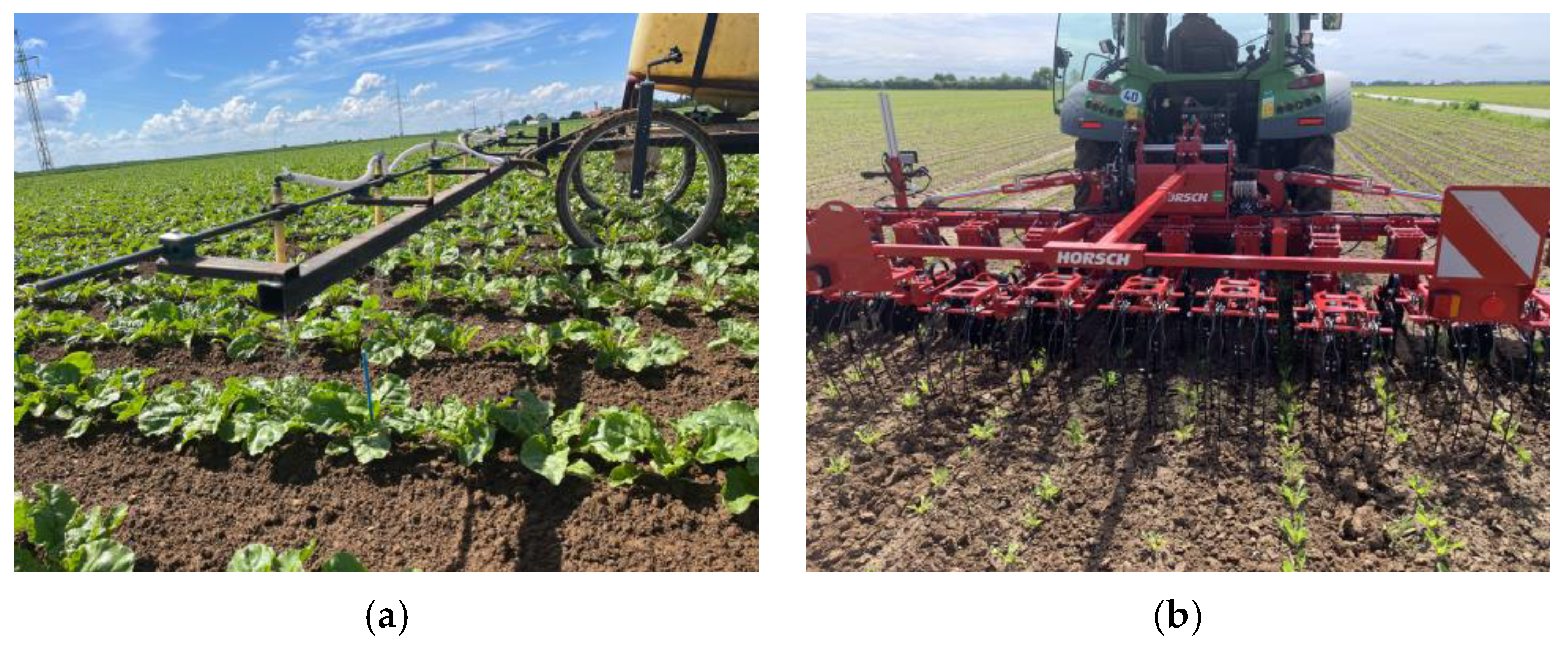
2.4. Experimental Implementation, Technology, and Machines

For interrow hoeing, a 12-row Horsch Model ‘Transformer 6 VF’, manufactured in 2022 with a working width of 6 m, was used, and rear mounted on a tractor (see Figure 1b). The machine was equipped with A blades (Model ‘EdgeOn’, without carbide for shallow cutting, three 15 cm blades for each interrow) and follow-up harrow units mounted on parallelograms without hydraulic downforce for weed control between the rows (interrow). Interrow hoeing was carried out with a working width interrow of 34 cm and was steered by a camera guidance system (Culticam) using a hydraulic side shift. For the hoeing operations at the first post-em., crop protection discs prevented soil from covering the still-small sugar beet plants. Precise hoeing passes were achieved at a constant speed of 3 km/h for the first post-em. and 8 km/h for the second and third post-em. A mechanical depth adjustment allowed an incremental increase in working depth by 2 cm per pass from the first to the third post-em., ensuring optimal machine settings for effective hoeing operations. No mechanical weed control was performed within the sugar beet rows (intrarow). Herbicide applications were carried out using a custom-built, electromotorized plot sprayer with a working width of 3 m, operating at a spray pressure of 2.5 bar and a working speed of 4 km/h (see Figure 1a). For broadcast spraying applications, the sprayer was equipped with low-drift injector flat fan nozzles (Model: Agrotop, size 02) with a 110° spray angle. In treatments involving herbicide band applications (band/hoe), the sprayer was fitted with specialized narrow-angle injector flat fan nozzles (Model: Agrotop, size 01) with a 40° spray angle. Since overlapping adjacent nozzles is not feasible in band spraying, these low-drift nozzles ensured a uniform distribution of active ingredients of herbicides across the entire width of the spray band over the beet rows. The spray band width was consistently set to 25 cm for all band applications.
For all herbicide applications, a herbicide mixture targeting the site-specific standard weed spectrum was used. The mixture contained the active ingredients metamitron, quinmerac, ethofumesate, phenmedipham, and an adjuvant and clopyralid. The water application rate was 240 L/ha for broadcast herbicide applications and 120 L/ha for herbicide band applications, adjusted to the spray band width of 25 cm, so that the same amount of herbicidal active ingredients could be applied per square meter of actually treated area. More detailed information, including specific application rates for each post-emergence application (post-em.), can be found in Table 3.

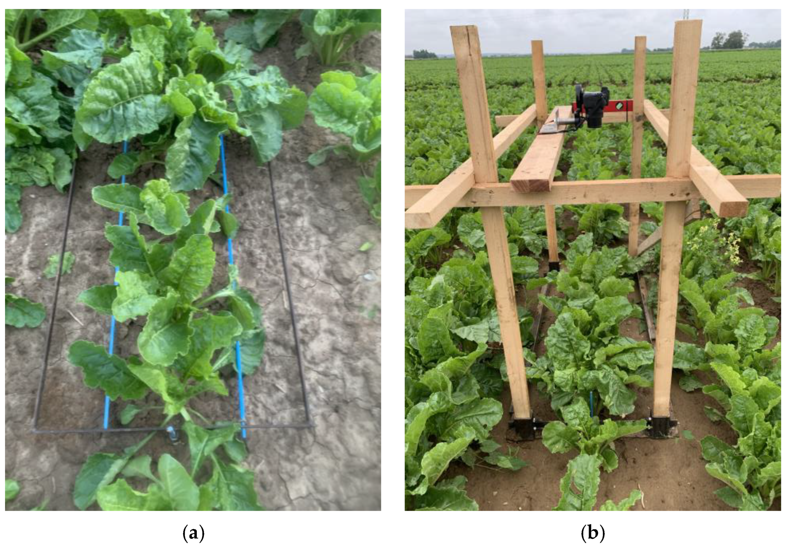
2.5. Data Acquisition—Weed Density and Weed Cover

In each plot, three weed assessment areas were measured at 2 m intervals and marked with field rods. Each assessment area had a size of 0.5 × 1 m (0.5 m2). To eliminate edge effects and track effects from machine operations, the assessment areas were placed in the seventh sugar beet row of each plot, maintaining a distance of 4.5 m from the short plot edges. To quantify the weed control efficacy of the different treatment combinations, two methods were used. First, five days after the third post-emergence application (post-em.), the weed density within each weed assessment area was determined using a modified Göttinger counting frame [30], precisely matching the size of the weed assessment area (0.5 m × 1 m = 0.5 m2) (see Figure 2a). The counting frame was divided into area-identical interrow and intrarow sections, allowing separate evaluation of weed density and weed control efficacy between the sugar beet rows (interrow) and directly within the sugar beet rows (intrarow). In each plot, a total of 1.5 m2 (0.75 m2 interrow, 0.75 m2 intrarow) was assessed. Second, 14 days after the third post-em., photographic recordings were taken for subsequent image analysis to determine the weed cover within the weed assessment areas. In the first experimental year (2023), a Nikon D80 DSLR camera (effective resolution: 10.2 MP) was mounted on a tripod and positioned 90 cm horizontally above the ground to capture images. The tripod was equipped with a frame identical in size to the counting frame (0.5 m × 1 m = 0.5 m2) (see Figure 2b). In the second experimental year (2024), a mirrorless Canon EOS R50 camera (effective resolution: 24.2 MP) was used for image acquisition. In both years, images were taken with a fixed focal length of 18 mm.

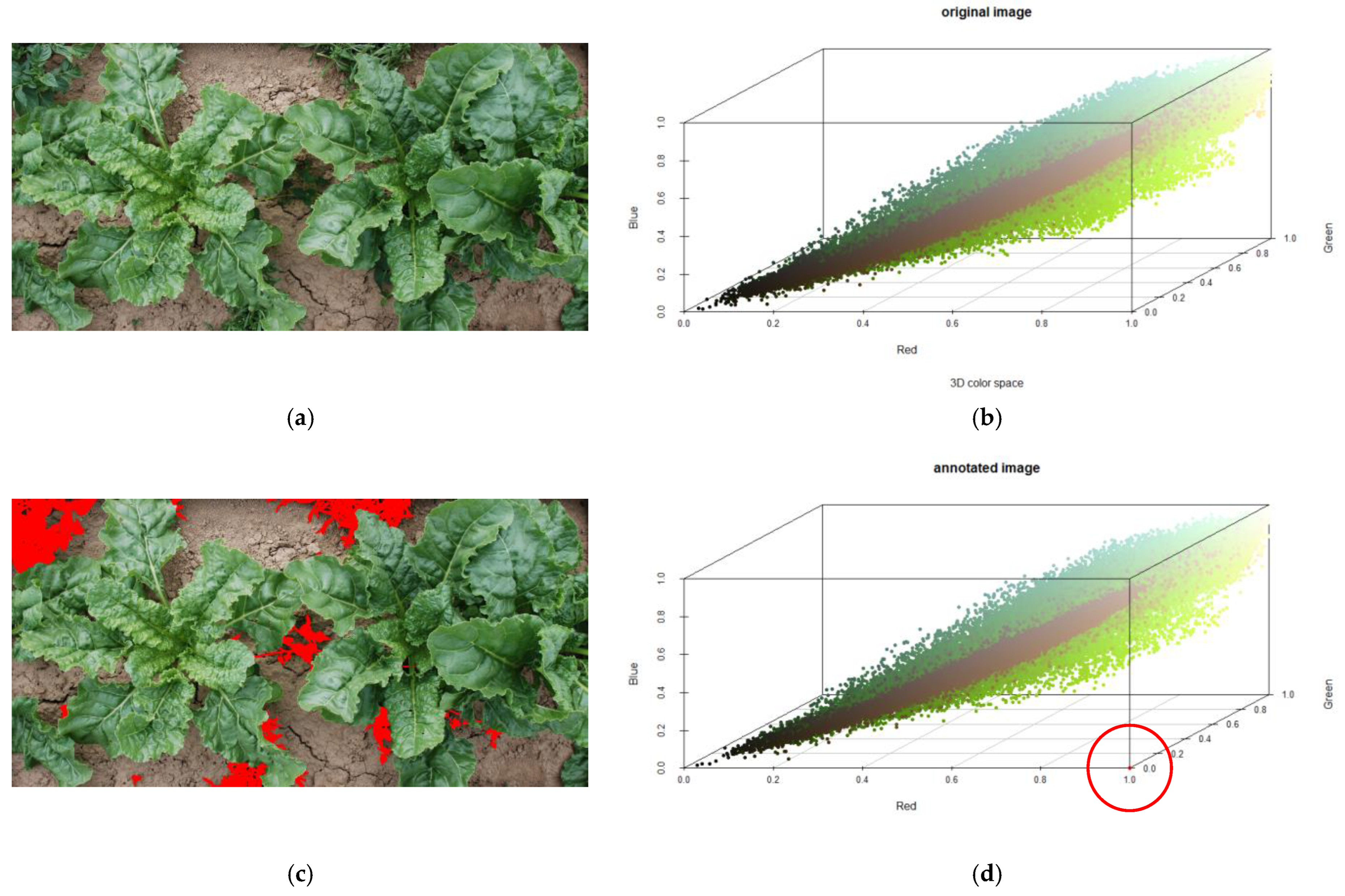
2.6. Data Processing and Statistical Analysis

For the calculation of the weed control efficacy of the treatments, the weed density (1) and the weed cover (2) after the third post-emergence application (post-em.) were calculated in relation to the untreated control (treatment 1) using the following formulas:
( W e e d   d e n s i t y u n t r e a t e d ) ( W e e d   d e n s i t y t r e a t m e n t   i ) ( W e e d   d e n s i t y u n t r e a t e d ) 100 = W e e d   c o n t r o l   e f f i c a c y ( W C E ) t r e a t m e n t   i [ % ]
( W e e d y   p i x e l s u n t r e a t e d ) ( W e e d y   p i x e l s t r e a t m e n t   i ) ( W e e d y   p i x e l s u n t r e a t e d ) 100 = W e e d   c o n t r o l   e f f i c a c y ( W C E ) t r e a t m e n t   i [ % ]
The images generated after the third post-em. to determine the weed cover in the weed assessment area were first centered using standard image processing programs and cropped to a uniform size (2023: 3145 × 1615 pixels; 2024: 5390 × 2700 pixels) to exclude edge effects. Using the software IrfanView (64 4.62) [31], the weeds in each photo were hand-annotated with a fixed color (RGB = 1, 0, 0). The final determination of the number of hand-annotated pixels was carried out using the software RStudio, Version 2024.09.1-349 (pkg.: countcolors, colordistance, png, writexl) [32,33,34,35,36]. The ratio of the number of manually annotated pixels (weeds) to the total number of pixels in the corresponding image results in the weed cover percentage for each weed assessment area. Figure 3 outlines the procedure. Image (a) shows a cropped image and its corresponding RGB color space (b) before manual annotation. Images (c) and (d) reflect the result after manual annotation. In (d), a single red data point is visible at RGB (1, 0, 0), which represents all of the red pixels annotated in image (c). This visual verification ensured the accuracy of the calculations, preventing any additional pixels in the RGB range of (1, 0, 0) from being mistakenly included.
Statistical analyses and graphical data presentations were also performed using RStudio, Version 2024.09.1-349 (pkg.: agricolae, base, ggpubr, ggplot2) [32,37,38,39,40]. Data were converted to the unit of one square meter and tested for normal distribution and heteroscedasticity. Statistical tests for significant differences between the experimental treatments were conducted using a one-way analysis of variance (ANOVA). To identify statistically significant differences, the Tukey HSD test was applied for post hoc analysis.

3. Results

In the first experimental year (2023), Chenopodium album and Polygonum convolvulus were the predominant weed species, while in 2024, Gallium aparine and Polygonum amphibium were the dominant weeds during the assessments. These species are considered typical site-specific weeds in sugar beet cultivation at the trial locations. Furthermore, it should be noted that herbicide-resistant weeds did not play a role on the trial sites.

3.1. Weed Density and Weed Control Efficacy

Table 4 presents the results of weed density within the weed assessment areas after the third post-em., as well as the corresponding weed control efficacy (WCE) in relation to the untreated control (treatment 1) for both experimental years. In addition to displaying countings within the entire weed assessment area (total), the division of the Göttinger counting frame allows area-identical differentiation between the areas between the sugar beet rows (interrow) and within the rows (intrarow), in order to specifically examine the weed control performance of the combinations of band spraying and hoeing, as well as hoeing alone (treatments 10–15), in relation to specific working areas.
Notably, there was a striking difference in weed growth between the years. While in the first experimental year (2023), the untreated control (treatment 1) had an average of 39.84 weeds/m2 across the entire weed assessment area, and the weed density in the untreated control in 2024 was 19.34 weeds/m2, representing a 2.06-fold reduction compared to the previous year. However, it is evident that treatment 1 consistently showed a higher weed density compared to all other treatments, meaning that all procedure combinations achieved weed control performance. In a more detailed evaluation of the interrow area (2023), treatment 1 had an average weed density of 54.00 weeds/m2, which was significantly higher than all other treatments. The statistical analysis did not show significant differences between treatments 2 to 15. The lowest weed density of 5.00 weeds/m2, and, thus, the highest WCE, of 90.74% compared to the untreated control, was observed in treatment 5 (b/h–b/h–br). For the intrarow area (2023), the untreated control had the highest weed density of 25.67 weeds/m2. The following significance level included treatments 8 and 9, and 11 to 15. These did not demonstrate clear, significant differences in weed density (intrarow) between the untreated control and the remaining treatments. Treatments 2 to 7 and 10 had significantly lower weed density compared to the untreated control. Treatment 7 (b/h–br–b/h) displayed the highest weed control efficacy in the intrarow area, with a value of 1.00 weeds/m2 and a corresponding WCE of 96.10%. In terms of total weed densities and WCEs without differentiation between inter- and intrarow areas in 2023, treatment 1 exhibited a significantly higher weed density of 39.84 weeds/m2 compared to all other treatments. Treatment 14 (h–b/h–br) had 15.34 weeds/m2 and a WCE of 61.50%, which did not reach clear significance in terms of weed density (total) in comparison to all other observations. Treatments 2 to 13 and 15 did not show significant differences in terms of weeds/m2 in 2023 between each other, but a significantly lower weed density compared to treatment 1. Treatment 7 (b/h–br–b/h) resulted in the lowest weed density of 3.67 weeds/m2 and the highest WCE of 90.80%.
In the interrow area in 2024, the untreated control (treatment 1) had a value of 24.00 weeds/m2, significantly differing from all treated ones. Treatments 3 to 5, 7 to 9, and 13 and 14 formed the next level with significantly lower weed density in comparison to treatment 1, but with higher weed density without clear significant distinction compared to all other treated observations. The group with the lowest level of weeds/m2 and the highest WCEs in the interrow area 2024 included treatments 2, 6, 10 to 12, and 15. Treatment 10 (br–b/h–h) had a value of 0.33 weeds/m2 and a WCE of 98.63%, making it the most effective weed control combination. In the intrarow area in 2024, all treatments showed lower weed density compared to the untreated control. Treatments 4, 6 to 8, and 13 and 14 showed lower weed density compared to treatment 1 and were grouped without clear differentiation compared to all other treatments. Treatments 2, 3, 5, 9 to 12, and 15 had significantly lower weed densities than treatment 1, ranging from 1.00 to 4.00 weeds/m2. Treatment 5 (b/h–b/h–br) achieved the highest WCE at 93.18%. Without differentiation between the interrow and intrarow areas (total), the untreated control also had the significantly highest weed density of 19.34 weeds/m2 in 2024. Treatment 14 (h–b/h–br) resulted in significantly lower weed density compared to treatment 1 and the highest weed density and lowest WCE in comparison to other treatments. Treatments 3, 4, 6 to 9, and 13 showed significantly lower weed densities compared to treatment 1, but no clear significant differences from all other treated ones. Treatments 2, 5, 10 to 12, and 15 had significantly lower weed densities and higher WCEs in comparison to the untreated control and treatment 14 (h–b/h–br). Treatment 10 (br–b/h–h) with a weed density of 1.83 weeds/m2 and a WCE of 90.54% was identified as the most effective weed control combination. In all evaluations, all treated combinations showed a strikingly lower weed density per square meter compared to the untreated control. It is noteworthy that combinations of mechanical and herbicide weed control methods achieved comparable or, in some cases, better weed control performance compared to solo broadcast herbicide applications.

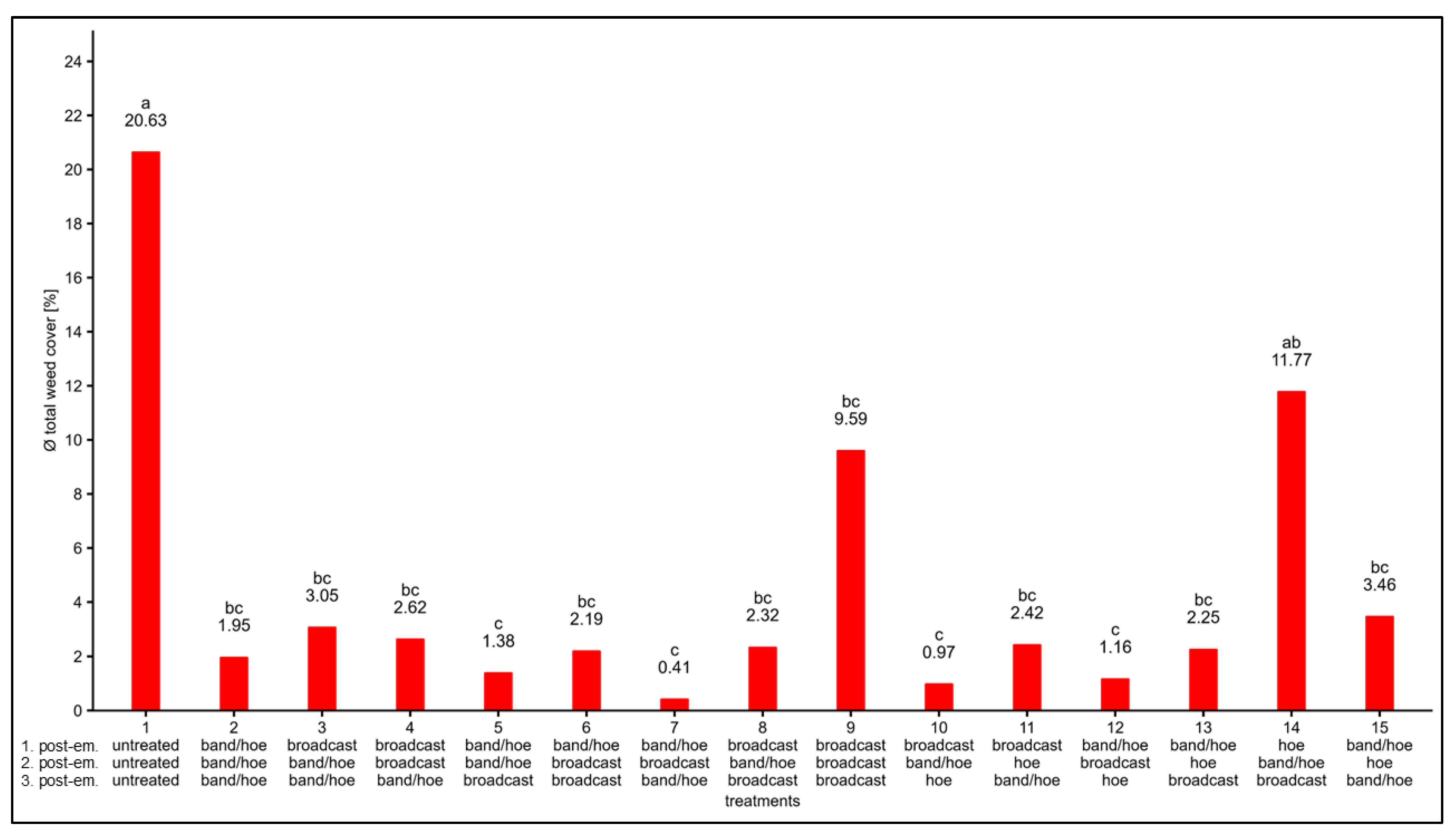
3.2. Weed Cover and Weed Control Efficacy

In both experimental years, two weeks after the third post-em., the weed cover percentage within each weed assessment area was determined through image analysis. Unlike the absolute weed density, this analysis did not differentiate between the interrow and intrarow areas.
The results indicate that the untreated control treatment 1 had the highest average weed cover percentage in both years, at 20.63% in 2023, and a strikingly lower value of 1.98% in 2024. This substantial reduction reflects the generally lower weed pressure in 2024. Figure 4 presents the average weed cover percentage for the 2023 trial year according to the different weed control combinations applied. Treatment 14 (h–b/h–br) exhibited the second-highest weed cover at 11.77%, lower than the untreated control but significantly higher than treatments 5, 7, 10, and 12 and without clearly significant difference compared to treatments 1–4, 6, 8, 9, 11, 13, and 15. The purely herbicide weed control strategy (treatment 9, br–br–br) achieved a significantly lower weed cover percentage of 9.59% compared to treatment 1, but did not achieve the same efficacy of the remaining treatments with no clear significant differences. The most effective treatments in 2023 were those integrating mechanical and herbicidal weed control, except treatment 14 with solo hoeing at the first post-em. Treatment 7 (b/h–br–b/h) had the lowest weed cover at 0.41%, followed closely by treatment 5 (b/h–b/h–br) at 1.38%. These two, as well as treatments 10 and 12, exhibited the lowest weed cover compared to all other treatments, but without any significant difference to treatments 2–4, 6, 8, 9, 11, 13, and 15 and with significantly lower weed cover compared to treatments 1 and 14.
In 2024 (Figure 5), the weed cover was dramatically reduced across all treatments compared to 2023. Treatment 1 resulted in significantly higher weed cover at 1.98%. All treated variants achieved significantly lower weed cover than the untreated control, with no significant differences between them. Treatment 14 (h–b/h–br) again had the highest weed cover among treated observations and resulted in a weed cover of 0.71%, while the purely herbicide treatment 9 (br–br–br) exhibited significant improvements in weed control comparison between the treatments, achieving a weed cover percentage of 0.14% in 2024. The best-performing treatment was 11 (br–h–b/h), with an exceptionally low weed cover value of 0.01%.
These results indicate that combinations of mechanical–chemical weed control strategies can provide weed cover percentages equal to or even lower than those of solo broadcast herbicide applications and therefore are consistent with the experimental hypothesis.
In order to assess the respective weed control efficacy of the treatments in both trial years in more detail using image analysis, the average number of annotated pixels for each weed control treatment was set in relation to the corresponding number of annotated pixels for the untreated control (Table 5). In 2023, treatment 14 (h–b/h–br) exhibited the lowest WCE of 42.94%. Treatment 9 with solo broadcast herbicide application (br–br–br) achieved a WCE of 53.52% compared to treatment 1. Combinations of mechanical and herbicidal weed control ranked in a range from 83.25% for treatment 15 (b/h–h–b/h) to 98.02% for treatment 7 (b/h–br–b/h). The results from 2024 show that treatment 14 (h–b/h–br) again achieved the lowest weed control success among all treatments with a WCE of 63.99% in relation to the untreated control. Treatment 9 (br–br–br) resulted in a WCE of 93.17%, thus showing better weed control performance in comparison to all treatments than in the previous year. The WCE of the other treatments ranged from 80.31% for treatment 13 (b/h–h–br) to 99.5% for treatment 11 (br–h–b/h).

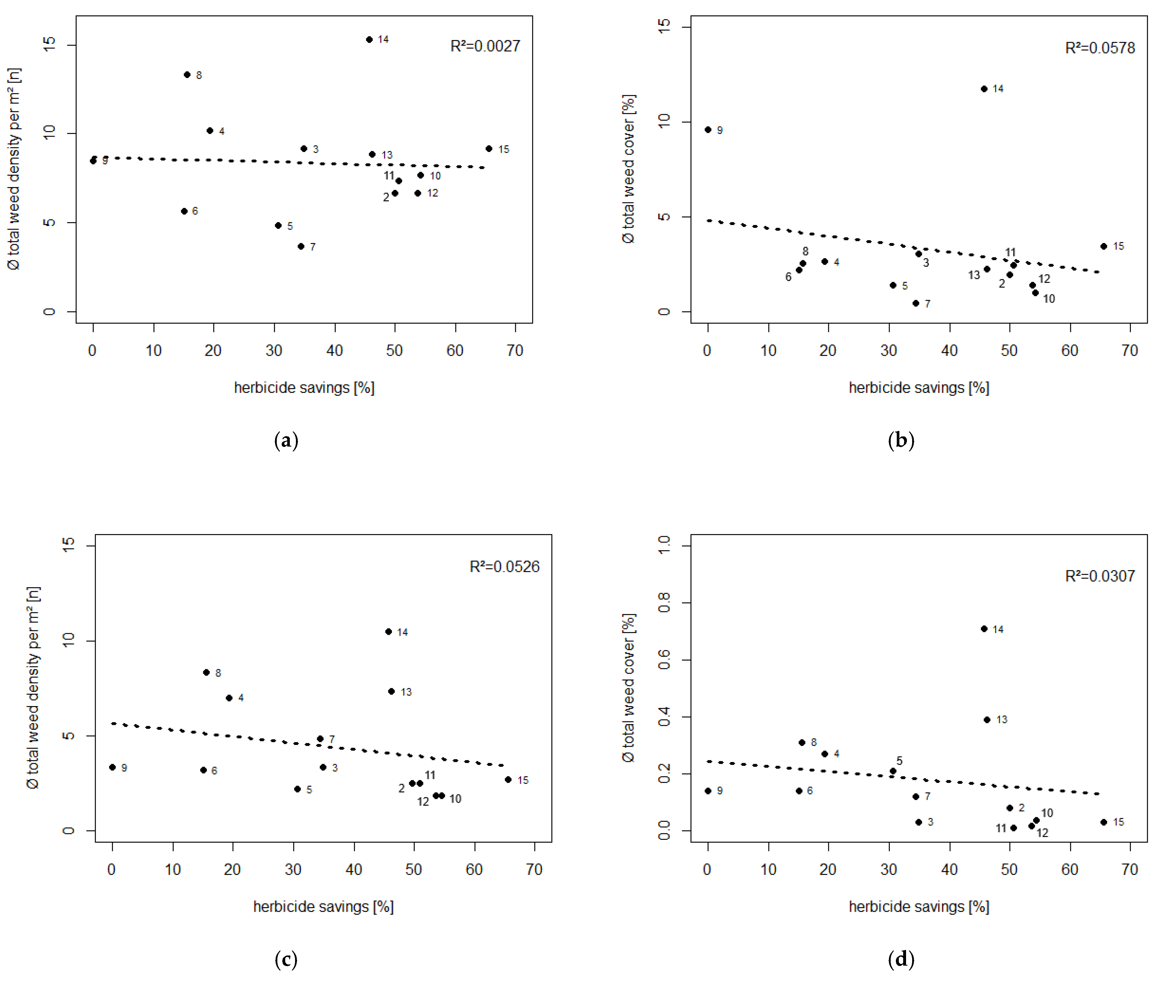
3.3. Correlation Analysis—Weed Density and Weed Cover to Herbicide-Saving Potential

An interesting question arises as to what extent the weed density and weed cover correlate with the respective herbicide-savings potential. Figure 6 presents the results of a simple correlation analysis between the treatment-dependent herbicide savings relative to the broadcast herbicide application and the total weed density per m2, as well as weed cover for treatments 2 to 15 in 2023 (a, b) and 2024 (c, d). Black trend lines and coefficients of determination illustrate the results of the linear correlation.
From all analyses, it is evident that weed density and weed cover do not follow a linear correlation with herbicide savings across all treated variants. All calculated coefficients of determination are below R2 = 0.1. This indicates that neither weed density nor weed cover increased linearly with higher herbicide savings in the treated variants in this study.

4. Discussion

4.1. Discussion of the Site Selection and Methods

In this study, fifteen treatments were selected to determine at which time points within three post-em. weed control operations in sugar beet herbicide broadcast applications could be omitted and replaced by a combination of herbicide band application intrarow and mechanical hoeing interrow or by mechanical hoeing interrow alone while still achieving high weed control efficacy alongside herbicide savings. To achieve this, a two-year field experiment was conducted in a high-intensity sugar beet cultivation region in Lower Bavaria, southeastern Germany. Due to the relatively large working widths of the machines used in the experiment, each plot was established at 96 m2 (6 m × 16 m). This setup proved advantageous as it effectively eliminated wheel track and edge effects while ensuring standardized driving speeds during machine operations. However, given the heterogeneous distribution of weeds in agricultural fields [41,42,43], large plot sizes can pose challenges in determining weed control efficacy. Nevertheless, through randomization of the plot layout and assessments conducted within fixed, marked weed assessment areas, a meaningful evaluation of the control performance of individual treatments was achieved.
Statistical analyses revealed that neither weed density nor weed cover data followed a normal distribution. Despite this, a one-way ANOVA with a subsequent Tukey-HSD post hoc test was conducted as a parametric method in the further analysis process. This decision was made because non-parametric rank-sum tests, such as the Kruskal–Wallis test, were found to be unsuitable, particularly for the weed counting data. The datasets for individual treatments contained numerous tied ranks. Blanca et al. [44] describe the applicability of a one-way ANOVA, even in cases of violated normality assumptions. Since all calculations included equal sample sizes as well as sample sizes greater than 10 (n > 10), the ANOVA can still be considered robust [45,46,47].
To assess weed control efficacy, two methods were applied. First, absolute weed counts were conducted using a modified Göttinger counting frame to evaluate weed density after the third post-em. weed control measure. This manual method is considered an accurate way to capture the existing weed density over an area covered by the counting frame [30,48]. The counting frame was divided into two equally sized sections, distinguishing between the area between the sugar beet rows (interrow) and the area within the rows (intrarow). This differentiation allowed an assessment to be made of the weed control efficacy of the individual control strategies and was particularly necessary since the combination of mechanical and herbicide weed control methods operates in different working zones. Nevertheless, the width of the herbicide band application intrarow was 25 cm. The width of the mechanical weed control in the interrow area was set to 34 cm. This results in an overlap of 4.5 cm on both sides of each sugar beet row when applying the band/hoe system, in which present weeds were controlled both mechanically and chemically. This approach is not optimal for the separate assessment of weed densities in the interrow and intrarow areas. However, the experimental setup was aligned with the machine settings commonly used in the region to support the practical applicability of the methods. In future trials, it should be examined whether the width of the herbicide band application could be reduced while maintaining the width of the hoeing area interrow, in order to achieve smaller overlap zones and further herbicide savings. Additionally, the counting frame could be divided into a third zone corresponding to the overlap area, allowing for a more detailed assessment of weed control efficacy within the different working areas of the band/hoe system. Second, the determination of absolute weed density was supplemented with an image analysis of weed cover after the third post-em. weed control measure. Without this methodological approach, a comparison between mechanical or combined mechanical–chemical weed control methods and solo broadcast herbicide applications would be difficult to achieve. While solo herbicide weed control inhibits or prevents further weed growth, ultimately leading to their decay [49,50], mechanical control methods have an immediate effect by cutting, uprooting, or burying weeds [51]. Therefore, an evaluation of the weed control efficacy of the different treatments based only on counted weed density may insufficiently capture the comparison between purely herbicidal and mechanical or mechanical–chemical control strategies.

4.2. Discussion of the Results

In all treated variants, lower weed density and weed cover were observed compared to the untreated control. The weed-counting results align with the findings of Kunz et al. [14] in sugar beet. They investigated, among other factors, mechanical–chemical and solo chemical weed control combinations, which correspond to treatments 2 (b/h–b/h–b/h), 3 (br–b/h–b/h), and 9 (br–br–br) in this study. Furthermore, in their weed density assessments, they observed no significant differences between these treatments in any of their observations [14]. This aligns with the results of the present study for the 2023 trial year. However, in 2024 in this study, the combination of three successive band/hoe applications (treatment 2) achieved a level of lower weed density compared to treatment 3 and the solo broadcast herbicide application (treatment 9). The combinations of herbicide band application on the sugar beet rows (intrarow), mechanical hoeing between the sugar beet rows (interrow), and broadcast herbicide application within three post-emergence applications demonstrated excellent weed control performance under both high and low weed pressure. Compared to the solo broadcast herbicide application, the combined mechanical–chemical weed control methods investigated in this study achieved similar or even superior weed control efficacies. For this reason, the hypothesis, ‘The use of mechanical–chemical combinations for weed control in three post-emergence applications in sugar beet results in similar weed control efficacy compared to solo broadcast herbicide spraying’, can be confirmed. Kunz et al. [14] and Wiltshire et al. [52] also reported similar or even higher weed control efficacies of the band sprayer/hoe combination compared to the solo broadcast herbicide application in sugar beet. Nevertheless, it is important to note that both the area between the sugar beet rows (interrow) and within the rows (intrarow) must be treated for weed control during the first post-em. Treatment 14, where only mechanical hoeing between the rows was performed during the first post-em., followed by a band/hoe combination and a broadcast herbicide application, stands out as the treatment with the lowest total WCE among all treated variants, both for weed count and for assessments using image analysis. It can be concluded that a solo hoeing measure between the rows during the first post-em. leads to a low total WCE. By the second post-em., the weeds within the rows had advanced too far in their growth to be controlled effectively with a band/hoe combination followed by a broadcast herbicide application at the third post-em. Larger weeds cannot be sufficiently controlled with applications of standard herbicides [15]. This means that for the first post-em., weeds must be controlled both in the interrow area and within the rows. Looking at the WCEs of the other treatments, it is important to clarify that, in this study, it did not matter whether this control was carried out through a combination of herbicide band spraying and mechanical hoeing or a broadcast herbicide application for the first post-em. as, in both cases, the weeds within the row were controlled with herbicides. Therefore, the use of herbicides remains crucial for the success of weed control in sugar beet, especially in the area within the crop rows (intrarow).
To further evaluate the relationship between herbicide savings and weed control performance in all weed-control treatments in this study, correlation analyses were conducted between weed density and weed cover in terms of treatment-specific herbicide savings. The results showed that there was no linear correlation between weed density and weed cover in relation to treatment-specific herbicide savings. In general, weed density and weed cover did not increase with increasing herbicide savings of the combinations. This again reflects the comparable, or even higher, weed control efficacy of mechanical–chemical weed control combinations in this study compared to the solo broadcast herbicide application. Other studies confirm the high weed control efficacies of mechanical–chemical combinations in sugar beet [17,53,54]. Moreover, the higher or comparable weed control efficacies of mechanical–chemical combinations compared to solo broadcast herbicide applications are also well documented in other field crops such as maize, winter wheat, sunflowers, carrots, and potatoes [55,56,57,58,59,60].
In many studies, weed control efficacy is determined based on weed counting in relation to the untreated control without weed control. To compare weed control efficacies between purely chemical and mechanical or mechanical–chemical management strategies, an additional assessment of weed cover using image analysis seems beneficial. This is an important parameter in the context of evaluating weed control strategies in sugar beet [7]. This is evident when comparing the individual WCEs from weed counts using the Göttinger counting frame (Table 4) and the calculated WCEs from image analysis showing weed cover (Table 5) in this study. While the total WCE for the three-fold, solo broadcast herbicide application (treatment 9) in 2023 was 78.66% based on weed counts, the WCE from image analysis showed only 53.52%. This suggests that, while a large portion of the weeds was effectively controlled by this treatment in 2023, some weeds were inadequately controlled, allowing their growth to continue to a limited extent. A few weeds, in this case, caused a disproportionately higher level of weed cover compared to the other treatments, which was not fully captured when only considering the results from weed counting.
Mechanical weed control methods within the crop rows (intrarow) usually achieve lower weed control efficacy or higher weed density compared to herbicide application [14,53,61]. For mechanical weed control, camera-guided hoeing devices are preferred over standard hoeing machines without camera-based control due to higher working speeds, reduced crop damage, and increased weed control efficacy [14,62]. It is important to note that the implementation of mechanical weed control methods in general is labor-intensive and requires optimal timing of application, and its effectiveness is typically highly dependent on weather conditions [14,15,63]. The weed control efficacy of mechanical weed control measures can decrease due to regrowth under wet soil conditions [15,64].

5. Conclusions

Effective weed control is essential for successful sugar beet cultivation. The combination of mechanical, mechanical–chemical, and broadcast herbicidal methods for weed control in three post-emergence applications can achieve both successful weed control and considerable herbicide savings. The results of this study demonstrate high weed control efficiencies for the mechanical–chemical combinations investigated. Furthermore, the results highlight the necessity of effective weed control within the beet rows (intrarow) during the first post-emergence application. Any deficiencies at this stage cannot be corrected by broadcast chemical or mechanical–chemical combinations used in subsequent post-emergence applications. No linear relationship could be found between herbicide savings and the absolute weed density or weed cover. The mechanical–chemical weed control combinations investigated in this study resulted in weed control efficacies comparable to or even higher than those of solo broadcast herbicide application in post-emergence measures and achieved herbicide savings of up to 65.59%.

Author Contributions

Conceptualization, J.B. and H.R.; methodology, J.B.; investigation, J.B.; data curation, J.B.; writing—original draft preparation, J.B.; writing—review and editing, H.R. and H.B. All authors have read and agreed to the published version of the manuscript.

Funding

This research was funded by the Association of Bavarian Sugarbeet Growers e.V., Sandstr. 4, 93092 Barbing, GER. The scientific work was linked to the project “Praxiseinführung von Verfahren mit reduziertem Pflanzenschutzmitteleinsatz im Zuckerrübenanbau—PraxPSMZR” (L/a-7342.3-1/44/10), funded by the Bavarian State Ministry of Food, Agriculture, Forestry, and Tourism.

Data Availability Statement

The data presented in this study are available from the corresponding author on reasonable request.

Acknowledgments

We would like to thank the Arbeitsgemeinschaft zur Förderung des Zuckerrübenanbaues (ARGE) Regensburg for their support in conducting work and assessments.

Conflicts of Interest

The authors declare no conflicts of interest.

Abbreviations

The following abbreviations are used in this manuscript:
post-em.post-emergence application
b/hband/hoe
hhoe
brbroadcast
Nnitrogen

References

  1. Bruhns, J.; Bruhns, P. Sugar Economy Europe, 71st ed.; Verlag Dr. Albert Bartens KG: Berlin, Germany, 2025; p. 17. ISBN 978-3-87040-196-2. [Google Scholar]
  2. Varga, I.; Jović, J.; Rastija, M.; Markulj Kulundžić, A.; Zebec, V.; Lončarić, Z.; Iljkić, D.; Antunović, M. Efficiency and Management of Nitrogen Fertilization in Sugar Beet as Spring Crop: A Review. Nitrogen 2022, 3, 170–185. [Google Scholar] [CrossRef]
  3. Kotlánová, B.; Hledík, P.; Hudec, S.; Martínez Barroso, P.; Vaverková, M.D.; Jiroušek, M.; Winkler, J. The Influence of Sugar Beet Cultivation Technologies on the Intensity and Species Biodiversity of Weeds. Agronomy 2024, 14, 390. [Google Scholar] [CrossRef]
  4. Scott, R.K.; Wilcockson, S.J.; Moisey, F.R. The effects of time of weed removal on growth and yield of sugar beet. J. Agric. Sci. 1979, 93, 693–709. [Google Scholar] [CrossRef]
  5. Bhadra, T.; Mahapatra, C.K.; Paul, S.K. Weed management in sugar beet: A review. Fundam. Appl. Agric. 2020, 5, 147–156. [Google Scholar] [CrossRef]
  6. Fishkis, O.; Koch, H.-J. Effect of mechanical weeding on soil erosion and earthworm abundance in sugar beet (Beta vulgaris L.). Soil Tillage Res. 2023, 225, 105548. [Google Scholar] [CrossRef]
  7. Gerhards, R.; Bezhin, K.; Santel, H.-J. Sugar Beet Yield Loss Predicted by Relative Weed Cover, Weed Biomass and Weed Density. Plant Protect. Sci. 2017, 53, 118–125. [Google Scholar] [CrossRef]
  8. Abd El Lateef, E.M.; Mekki, B.B.; Abd El-Salam, M.S.; El-Metwally, I.M. Effect of different single herbicide doses on sugar beet yield, quality and associated weeds. Bull. Natl. Res. Cent. 2021, 45, 21. [Google Scholar] [CrossRef]
  9. Kulan, E.G.; Kaya, M.D. Effects of Weed-Control Treatments and Plant Density on Root Yield and Sugar Content of Sugar Beet. Sugar Tech 2023, 25, 805–819. [Google Scholar] [CrossRef]
  10. Cioni, F.; Maines, G. Weed Control in Sugarbeet. Sugar Tech 2010, 12, 243–255. [Google Scholar] [CrossRef]
  11. Soltani, N.; Dille, J.A.; Robinson, D.E.; Sprague, C.L.; Morishita, D.W.; Lawrence, N.C.; Kniss, A.R.; Jha, P.; Felix, J.; Nurse, R.E.; et al. Potential yield loss in sugar beet due to weed interference in the United States and Canada. Weed Technol. 2018, 32, 749–753. [Google Scholar] [CrossRef]
  12. Kropff, M.J.; Spitters, C.J.T. A simple model of crop loss by weed competition from early observations on relative leaf area of the weeds. Weed Res. 1991, 31, 97–105. [Google Scholar] [CrossRef]
  13. Schweizer, E.E.; Dexter, A.G. Weed control in sugar beets (Beta vulgaris) in North America. Rev. Weed Sci. 1987, 3, 113–133. [Google Scholar]
  14. Kunz, C.; Weber, J.F.; Peteinatos, G.G.; Sökefeld, M.; Gerhards, R. Camera steered mechanical weed control in sugar beet, maize and soybean. Precis. Agric. 2018, 19, 708–720. [Google Scholar] [CrossRef]
  15. Petersen, J. A Review on Weed Control in Sugar Beet: From Tolerance Zero to Period Threshold. In Weed Biology and Management; Inderjit, Ed.; Kluwer Academic Publishers: Dordrecht, The Netherlands; Springer: Dordrecht, The Netherlands, 2004; pp. 467–483. [Google Scholar] [CrossRef]
  16. Roßberg, D.; Aeckerle, N.; Stockfisch, N. Erhebungen zur Anwendung von chemischen Pflanzenschutzmitteln in Zuckerrüben. Gesunde Pflanz. 2017, 69, 59–66. [Google Scholar] [CrossRef]
  17. Parasca, S.C.; Spaeth, M.; Rusu, T.; Bogdan, I. Mechanical Weed Control: Sensor-Based Inter-Row Hoeing in Sugar Beet (Beta vulgaris L.) in the Transylvanian Depression. Agronomy 2024, 14, 176. [Google Scholar] [CrossRef]
  18. Adamczewski, K.; Matysiak, K.; Kierzek, R.; Kaczmarek, S. Significant increase of weed resistance to herbicides in Poland. J. Plant Prot. Res. 2019, 59, 139–150. [Google Scholar] [CrossRef]
  19. Kalfa, A.-V.; Stuke, F.; Henneken, I.; Haberlah-Korr, V. Effizienz von Triazinon-haltigen Wirkstoffkombinationen zur Bekämpfung von Gänsefuß-Herkünften (Chenopodium album L.) mit verschiedenen Punktmutationen in Zuckerrübe. In Proceedings of the 29th German Conference on Weed Biology and Weed Control, Braunschweig, Germany, 3–5 March 2020; Nordmeyer, H., Ulber, L., Eds.; Julius Kühn-Institut: Braunschweig, Germany, 2020; pp. 360–366, ISBN 978-3-95547-088-3. [Google Scholar]
  20. Thiel, H.; Kluth, C.; Varrelmann, M. A new molecular method for the rapid detection of a metamitron-resistant target site in Chenopodium album. Pest Manag. Sci. 2010, 66, 1011–1017. [Google Scholar] [CrossRef]
  21. Duke, S.O. Why have no new herbicide modes of action appeared in recent years? Pest Manag. Sci. 2012, 68, 505–512. [Google Scholar] [CrossRef]
  22. Zwerger, P.; Augustin, B.; Becker, J.; Dietrich, C.; Forster, R.; Gehring, K.; Gerhards, R.; Gerowitt, B.; Huttenlocher, M.; Kerlen, D.; et al. Integriertes Unkrautmanagement zur Vermeidung von Herbizidresistenz*. J. Kult. 2017, 69, 146–149. [Google Scholar] [CrossRef]
  23. Kunz, C.; Schröllkamp, C.; Koch, H.-J.; Eßer, C.; Schulze Lammers, P.; Gerhards, R. Potentials of post-emergent mechanical weed control in sugar beet to reduce herbicide inputs. Landtechnik 2015, 70, 67–81. [Google Scholar] [CrossRef]
  24. Zawada, M.; Legutko, S.; Gościańska-Łowińska, J.; Szymczyk, S.; Nijak, M.; Wojciechowski, J.; Zwierzyński, M. Mechanical Weed Control Systems: Methods and Effectiveness. Sustainability 2023, 15, 15206. [Google Scholar] [CrossRef]
  25. Ghaly, A.E.; Ibrahim, M.M. Mechanization of Weed Management in Sugar Beet. In Sugar Beet Cultivation, Management and Processing; Misra, V., Srivastava, S., Mall, A.K., Eds.; Springer: Singapore, 2022; pp. 327–367. ISBN 978-981-19-2729-4. [Google Scholar]
  26. Tataridas, A.; Kanatas, P.; Chatzigeorgiou, A.; Zannopoulos, S.; Travlos, I. Sustainable Crop and Weed Management in the Era of the EU Green Deal: A Survival Guide. Agronomy 2022, 12, 589. [Google Scholar] [CrossRef]
  27. Triantafyllidis, V.; Mavroeidis, A.; Kosma, C.; Karabagias, I.K.; Zotos, A.; Kehayias, G.; Beslemes, D.; Roussis, I.; Bilalis, D.; Economou, G.; et al. Herbicide Use in the Era of Farm to Fork: Strengths, Weaknesses, and Future Implications. Water Air Soil Pollut. 2023, 234, 94. [Google Scholar] [CrossRef]
  28. IUSS Working Group WRB. World Reference Base for Soil Resources. International Soil Classification System for Naming Soils and Creating Legends for Soil Maps, 4th ed.; International Union of Soil Sciences (IUSS): Vienna, Austria, 2022; ISBN 979-8-9862451-1-9. [Google Scholar]
  29. Bayerische Landesanstalt für Landwirtschaft—Agrarmeteorologie Bayern. Wetterstation Piering (LfL). Download/Grafik. Available online: https://www.wetter-by.de/Internet/AM/NotesBAM.nsf/bamweb/bba59bec8619836fc12573920047005b?OpenDocument&TableRow=3.10#3 (accessed on 16 November 2024).
  30. Kluge, A. Methoden zur Automatischen Unkrauterkennung für die Prozesssteuerung von Herbizidmaßnahmen. In Dissertationen aus dem Julius Kühn-Institut; Julius Kühn-lnstitut, Federal Research Centre for Cultivated Plants, Ed.; Julius Kühn-Institut: Quedlinburg, Germany, 2011; ISBN 978-3-930037-77-3. [Google Scholar]
  31. Skiljan, I. IrfanView 64—Image Viewer. Software Version 4.62. Available online: https://www.irfanview.com (accessed on 12 June 2023).
  32. Posit Team. RStudio: Integrated Development Environment for R; Version: 2024.09.1-349; Posit Software, PBC: Boston, MA, USA, 2024; Available online: http://www.posit.co/ (accessed on 26 November 2024).
  33. Weller, H. countcolors: Locates and Counts Pixels Within Color Range(s) in Images; R Package Version 0.9.1; 2019. Available online: https://CRAN.R-project.org/package=countcolors (accessed on 26 November 2024).
  34. Weller, H. colordistance: Distance Metrics for Image Color Similarity; R Package Version 1.1.2; 2021. Available online: https://CRAN.R-project.org/package=colordistance (accessed on 26 November 2024).
  35. Urbanek, S. png: Read and Write PNG Images; R package version 0.1-8; 2022. Available online: https://CRAN.R-project.org/package=png (accessed on 26 November 2024).
  36. Ooms, J. writexl: Export Data Frames to Excel ‘xlsx’ Format; R Package Version 1.5.0; 2024. Available online: https://CRAN.R-project.org/package=writexl (accessed on 26 November 2024).
  37. De Mendiburu, F. agricolae: Statistical Procedures for Agricultural Research; R Package Version 1.3-7. 2023. Available online: https://CRAN.R-project.org/package=agricolae (accessed on 26 November 2024).
  38. R Core Team. R: A Language and Environment for Statistical Computing; R Foundation for Statistical Computing: Vienna, Austria, 2023; Available online: https://www.R-project.org/ (accessed on 26 November 2024).
  39. Kassambra, A. ggpubr: ‘ggplot2’ Based Publication Ready Plots; R Package Version 0.6.0; 2023. Available online: https://CRAN.R-project.org/package=ggpubr (accessed on 26 November 2024).
  40. Wickham, H. ggplot2: Elegant Graphics for Data Analysis, 2nd ed.; Use R! Gentleman, R., Hornik, K., Parmigiani, G., Eds.; Springer: New York, NY, USA, 2016; ISBN 978-3-319-24275-0. [Google Scholar]
  41. Kämpfer, C.; Nordmeyer, H. Teilflächenspezifische Unkrautbekämpfung als ein Baustein von Smart Farming. J. Kult. 2021, 73, 284–291. [Google Scholar] [CrossRef]
  42. Gerhards, R.; Andújar Sanchez, D.; Hamouz, P.; Peteinatos, G.G.; Christensen, S.; Fernandez-Quintanilla, C. Advances in site-specific weed management in agriculture—A review. Weed Res. 2022, 62, 123–133. [Google Scholar] [CrossRef]
  43. Kämpfer, C.; Ulber, L.; Wellhausen, C.; Pflanz, M. Unkrauterkennung und Kartierung zur automatischen Applikationskartenerstellung im Pflanzenschutz. J. Kult. 2021, 73, 121–130. [Google Scholar] [CrossRef]
  44. Blanca, M.J.; Alarcón, R.; Arnau, J.; Bono, R.; Bendayan, R. Non-normal data: Is ANOVA still a valid option? Psicothema 2017, 29, 552–557. [Google Scholar] [CrossRef]
  45. Bortz, J.; Schuster, C. Statistik für Human- und Sozialwissenschaftler, 7th ed.; Springer: Berlin/Heidelberg, Germany, 2010; p. 214. ISBN 978-3-642-12769-4. [Google Scholar]
  46. Glass, G.V.; Peckham, P.D.; Sanders, J.R. Consequences of Failure to Meet Assumptions Underlying the Fixed Effects Analyses of Variance and Covariance. Rev. Educ. Res. 1972, 42, 237–288. [Google Scholar] [CrossRef]
  47. Winer, B.J.; Brown, D.R.; Michels, K.M. Statistical Principles in Experimental Design, 3rd ed.; McGraw-Hill: New York, NY, USA, 1991; ISBN 978-0070709829. [Google Scholar]
  48. Pamornnak, B.; Scholz, C.; Becker, S.; Ruckelshausen, A. A digital weed counting system for the weed control performance evaluation. In Informatik in der Land-, Forst- und Ernährungswirtschaft: Künstliche Intelligenz in der Agrar- und Ernährungswirtschaft. Lecture Notes in Informatics (LNI)—Proceedings of the 42th GIL-Jahrestagung, Agroscope, Tänikon, Ettenhausen, Switzerland (Virtual), 21–22 February 2022; Gandorfer, M., Hoffmann, C., El Benni, N., Cockburn, M., Anken, T., Floto, H., Eds.; Köllen Druck+Verlag GmbH: Bonn, Germany, 2022; pp. 207–212. ISBN 978-3-88579-711-1. [Google Scholar]
  49. Das, S.K.; Mondal, T. Mode of action of herbicides and recent trends in development: A Reappraisal. Int. J. Agric. Soil Sci. 2014, 2, 27–32. [Google Scholar]
  50. Baćmaga, M.; Wyszkowska, J.; Kucharski, J. Environmental Implication of Herbicide Use. Molecules 2024, 29, 5965. [Google Scholar] [CrossRef]
  51. Hamed, L.M.M.; Absy, R.; Elmenofy, W.; Emara, E.I.R. Enhancing Sugar Beet (Beta vulgaris L.) Yield and Quality: Evaluating the Efficiency of Chemical and Mechanical Weed Control Strategies. Agronomy 2023, 13, 2951. [Google Scholar] [CrossRef]
  52. Wiltshire, J.J.J.; Tillett, N.D.; Hague, T. Agronomic evaluation of precise mechanical hoeing and chemical weed control in sugar beet. Weed Res. 2003, 43, 236–244. [Google Scholar] [CrossRef]
  53. Machleb, J.; Peteinatos, G.G.; Sökefeld, M.; Gerhards, R. Sensor-Based Intrarow Mechanical Weed Control in Sugar Beets with Motorized Finger Weeders. Agronomy 2021, 11, 1517. [Google Scholar] [CrossRef]
  54. Gerhards, R.; Risser, P.; Spaeth, M.; Saile, M.; Peteinatos, G. A comparison of seven innovative robotic weeding systems and reference herbicide strategies in sugar beet (Beta vulgaris subsp. vulgaris L.) and rapeseed (Brassica napus L.). Weed Res. 2024, 64, 42–53. [Google Scholar] [CrossRef]
  55. Loddo, D.; Scarabel, L.; Sattin, M.; Pederzoli, A.; Morsiani, C.; Canestrale, R.; Tommasini, M.G. Combination of Herbicide Band Application and Inter-Row Cultivation Provides Sustainable Weed Control in Maize. Agronomy 2020, 10, 20. [Google Scholar] [CrossRef]
  56. Saile, M.; Spaeth, M.; Gerhards, R. Evaluating Sensor-Based Mechanical Weeding Combined with Pre- and Post-Emergence Herbicides for Integrated Weed Management in Cereals. Agronomy 2022, 12, 1465. [Google Scholar] [CrossRef]
  57. Pannacci, E.; Tei, F. Effects of mechanical and chemical methods on weed control, weed seed rain and crop yield in maize, sunflower and soyabean. Crop Prot. 2014, 64, 51–59. [Google Scholar] [CrossRef]
  58. Main, D.C.; Sanderson, K.R.; Fillmore, S.A.E.; Ivany, J.A. Comparison of synthetic and organic herbicides applied banded for weed control in carrots (Daucus carota L.). Can. J. Plant Sci. 2013, 93, 857–861. [Google Scholar] [CrossRef]
  59. Ozaslan, C.; Gürsoy, S.; DiTommaso, A. Band herbicide application combined with inter-row cultivation as a sustainable weed management strategy for reducing herbicide use: A meta-analysis. Crop Prot. 2024, 175, 106474. [Google Scholar] [CrossRef]
  60. Ivany, J.A. Banded herbicides and cultivation for weed control in potatoes (Solanum tuberosum L.). Can. J. Plant Sci. 2002, 82, 617–620. [Google Scholar] [CrossRef]
  61. Melander, B.; Lattanzi, B.; Pannacci, E. Intelligent versus non-intelligent mechanical intra-row weed control in transplanted onion and cabbage. Crop Prot. 2015, 72, 1–8. [Google Scholar] [CrossRef]
  62. Machleb, J.; Peteinatos, G.G.; Kollenda, B.L.; Andújar, D.; Gerhards, R. Sensor-based mechanical weed control: Present state and prospects. Comput. Electron. Agric. 2020, 176, 105638. [Google Scholar] [CrossRef]
  63. Hussain, M.; Farooq, S.; Merfield, C.; Jabran, K. Mechanical Weed Control. In Non-Chemical Weed Control; Jabran, K., Chauhan, B.S., Eds.; Elsevier: Amsterdam, The Netherlands; Academic Press: San Diego, CA, USA, 2018; pp. 133–155. ISBN 978-0-12-809881-3. [Google Scholar]
  64. Bond, W.; Grundy, A.C. Non-chemical weed management in organic farming systems. Weed Res. 2001, 41, 383–405. [Google Scholar] [CrossRef]
Figure 1. (a) Plot sprayer for herbicidal band (intrarow) and broadcast applications. (b) Mechanical hoe for weed control between sugar beet rows (interrow).
Agronomy 15 00879 g001
Figure 2. (a) Modified Göttinger counting frame with 0.25 m2 interrow and intrarow counting spaces (sum = 0.5 m2). (b) Base-identical (0.5 m2) tripod for standardized photo recordings.
Agronomy 15 00879 g002
Figure 3. (a) Example photo of photo recordings for image analysis of weed cover prior to hand annotation (original image). (b) Three-dimensional color space corresponding to (a). (c) Example photo of photo recordings after hand annotation (annotated image). Weeds are annotated in red annotation color at RGB = (1, 0, 0) (d) Three-dimensional color space corresponding to (c), with a circle around red annotation color at RGB = (1, 0, 0).
Agronomy 15 00879 g003
Figure 4. Treatment (x-axis) and mean weed cover (y-axis) after the third post-emergence application in 2023. The individual weed control methods from the first to the third post-em. for each treatment are shown from top to bottom. Different letters show statistically significant differences in weed cover between trial treatments (Tukey, α = 0.05).
Agronomy 15 00879 g004
Figure 5. Treatment (x-axis) and mean weed cover (y-axis) after the third post-emergence application in 2024. The individual weed control methods from the first to the third post-em. for each treatment are shown from top to bottom. Different letters show statistically significant differences in weed cover between trial treatments (Tukey, α = 0.05).
Agronomy 15 00879 g005
Figure 6. (a) Correlation between herbicide savings of treatments 2 to 15 (x-axis) compared to treatment 9 (solo broadcast herbicide application) and mean weed density in 2023 (a) and 2024 (c) and mean weed cover in 2023 (b) and 2024 (d) (all y-axes). R2 = coefficient of determination. Numbers next to data points specify the corresponding treatment (see Table 2).
Agronomy 15 00879 g006
Table 1. Mean monthly weather conditions at the trial sites in the long-term average for 2012–2022 (top), 2023 (middle), and 2024 (bottom) from March to October [29].
Year(s)
Parameter
Mar.Apr.MayJun.Jul.Aug.Sep.Oct.∅ or Σ
2012–2022
Air temp. [°C]5.09.413.618.119.419.114.39.5∅ 13.6
Preci. [mm]31.228.879.293.152.478.151.048.4Σ 462.2
Veg.days [d]1625313031313029Σ 223
Soil temp. [°C]5.39.813.618.420.019.616.011.7∅ 14.3
2023
Temp. [°C]5.67.414.118.720.219.317.111.2∅ 14.2
Preci. [mm]41.572.546.817.459.3155.817.440.4Σ 451.1
Veg.days [d]1624313031313028Σ 221
Soil temp. [°C]5.98.612.417.819.519.117.312.7∅ 14.2
2024
Air temp. [°C]7.910.715.618.720.521.315.511.0∅ 15.2
Preci. [mm]15.827.4145.879.763.9117.7122.946.1Σ 619.3
Veg.days [d]2724313031313031Σ 235
Soil temp. [°C]7.811.115.318.620.620.317.013.0∅ 15.5
Notes: Air temp. = air temperature at 2 m height, Preci = precipitation sum, Veg.days = number of vegetation days, Soil temp. = soil temperature at 20 cm depth.
Table 2. Treatments with corresponding weed control method and herbicide savings (%) compared to solo broadcast herbicide application (treatment 9).
Treatment1. Post-em.2. Post-em.3. Post-em.Total Amount of
Applicated Herbicides
[L/ha]
Total Herbicide Savings [%]
Compared to Solo Broadcast (Treatment 9)
1untreateduntreateduntreated0.00100.00
2band/hoeband/hoeband/hoe4.6550.00
3broadcastband/hoeband/hoe6.0534.95
4broadcastbroadcastband/hoe7.5019.35
5band/hoeband/hoebroadcast6.4530.65
6band/hoebroadcastbroadcast7.9015.05
7band/hoebroadcastband/hoe6.1034.41
8broadcastband/hoebroadcast7.8515.59
9broadcastbroadcastbroadcast9.300.00
10broadcastband/hoehoe4.2554.30
11broadcasthoeband/hoe4.6050.54
12band/hoebroadcasthoe4.3053.76
13band/hoehoebroadcast5.0046.24
14hoeband/hoebroadcast5.0545.70
15band/hoehoeband/hoe3.2065.59
Notes: post-em. = post-emergence application.
Table 3. Post-em./BBCH depending on herbicide used with active ingredients, product name, and producer during both field trials in 2023 and 2024.
Post-em. BBCHActive IngredientsCTProduct NameFMARProducer
1. post-em.
10–11
Metamitron525 g/LGoltix TitanSC683 g/haAdama
Quinmerac40 g/LGoltix TitanSC52 g/haAdama
Ethofumesat190 g/LBetanal TandemSC190 g/haBayer Crop Sciences
Phenmedipham200 g/LBetanal TandemSC200 g/haBayer Crop Sciences
Rapeseed methyl ester810 mL/LMeroEC405 mL/haBayer Crop Sciences
2. post-em.
14
Metamitron525 g/LGoltix TitanSC683 g/haAdama
Quinmerac40 g/LGoltix TitanSC52 g/haAdama
Ethofumesat190 g/LBetanal TandemSC190 g/haBayer Crop Sciences
Phenmedipham200 g/LBetanal TandemSC200 g/haBayer Crop Sciences
Clopyralid600 g/LLontrelSC60 g/haCorteva
Rapeseed methyl ester810 mL/LMeroEC405 mL/haBayer Crop Sciences
3. post-em.
16–19
Metamitron525 g/LGoltix TitanSC1050 g/haAdama
Quinmerac40 g/LGoltix TitanSC80 g/haAdama
Ethofumesat190 g/LBetanal TandemSC190 g/haBayer Crop Sciences
Phenmedipham200 g/LBetanal TandemSC200 g/haBayer Crop Sciences
Clopyralid600 g/LLontrelSC60 g/haCorteva
Rapeseed methyl ester810 mL/LMeroEC405 mL/haBayer Crop Sciences
Notes: post-em. = post-emergence application, CT = concentration in product, FM = formulation, SC = suspension concentrate, EC = emulsifiable concentrate, AR = application rate.
Table 4. Trial treatments with corresponding herbicide savings (herb. savings), weed density (weed den.), and weed control efficacy (WCE) after the third post-emergence application for both trial years (2023 and 2024). Weed density and weed control efficacy are divided into the area between sugar beet rows (interrow), the area within sugar beet rows (intrarow), and both (total). Different letters after each weed density column indicate statistically significant differences in weed density between trial treatments (Tukey, α = 0.05).
Interrow 2023Intrarow 2023Total 2023Interrow 2024Intrarow 2024Total 2024
TreatmentHerb.
Savings
Weed
Den.
WCEWeed
Den.
WCEWeed
Den.
WCEWeed
Den.
WCEWeed
Den.
WCEWeed
Den.
WCE
Nr.1. Post-em.2. Post-em.3. Post-em.[%][n/m2][%][n/m2][%][n/m2][%][n/m2][%][n/m2][%][n/m2][%]
1untreateduntreateduntreated100.0054.00a -25.67a -39.84a -24.00a -14.67a -19.34a -
2band/hoeband/hoeband/hoe50.0010.00b81.483.33b87.036.67b83.271.00c95.834.00b72.732.50c87.07
3broadcastband/hoeband/hoe34.9512.67b76.545.67b77.919.17b76.983.67bc84.713.00b79.553.34bc82.75
4broadcastbroadcastband/hoe19.3514.67b72.835.67b77.9110.17b74.475.00bc79.179.00ab38.657.00bc63.80
5band/hoeband/hoebroadcast30.655.00b90.744.67b81.814.84b87.863.33bc86.131.00b93.182.17c88.80
6band/hoebroadcastbroadcast15.057.67b85.803.67b85.705.67b85.771.00c95.835.33ab63.673.17bc83.63
7band/hoebroadcastband/hoe34.416.33b88.281.00b96.103.67b90.802.33bc90.297.33ab50.034.83bc75.02
8broadcastband/hoebroadcast15.5914.33b73.4612.33ab51.9713.33b66.548.67bc63.888.00ab45.478.34bc56.89
9broadcastbroadcastbroadcast0.009.00b83.338.00ab68.848.50b78.663.67bc84.713.00b79.553.34bc82.75
10broadcastband/hoehoe54.3010.67b80.244.67b81.817.67b80.750.33c98.633.33b77.301.83c90.54
11broadcasthoeband/hoe50.548.00b85.196.67ab74.027.34b81.591.67c93.043.33b77.302.50c87.07
12band/hoebroadcasthoe53.767.33b86.436.00ab76.636.67b83.270.67c97.213.00b79.551.84c90.51
13band/hoehoebroadcast46.2410.33b80.877.33ab71.458.83b77.837.00bc70.837.67ab47.727.34bc62.06
14hoeband/hoebroadcast45.7015.00b72.2215.67ab38.9615.34ab61.5010.33bc56.9610.67ab27.2710.50b45.69
15band/hoehoeband/hoe65.5910.00b81.488.33ab67.559.17b76.991.33c94.464.00b72.732.67c86.22
Notes: nr. = treatment number, post-em. = post-emergence application.
Table 5. Trial treatments with corresponding herbicide savings (herb. savings), number of annotated pixels, and weed control efficacy (WCE) compared to untreated control (treatment 1) for both trial years (2023 and 2024).
20232024
TreatmentHerb.
Savings
Annotated
Pixels
WCEAnnotated
Pixels
WCE
Nr.1. Post-em.2. Post-em.3. Post-em.[%]n/m2[%]n/m2[%]
1untreateduntreateduntreated100.002,096,023--575,621--
2band/hoeband/hoeband/hoe50.00198,34690.5422,08596.16
3broadcastband/hoeband/hoe34.95310,11285.20761598.68
4broadcastbroadcastband/hoe19.35265,76187.3278,36186.39
5band/hoeband/hoebroadcast30.65140,26493.3157,58090.00
6band/hoebroadcastbroadcast15.05222,04989.4141,31492.82
7band/hoebroadcastband/hoe34.4141,57498.0235,74093.79
8broadcastband/hoebroadcast15.59236,14088.7390,86084.22
9broadcastbroadcastbroadcast0.00974,27853.5239,32893.17
10broadcastband/hoehoe54.3098,26395.31737498.72
11broadcasthoeband/hoe50.54245,65188.28290299.50
12band/hoebroadcasthoe53.76117,53194.39723598.74
13band/hoehoebroadcast46.24228,51389.10113,32880.31
14hoeband/hoebroadcast45.701,195,89542.94207,27663.99
15band/hoehoeband/hoe65.59350,98183.25819098.58
Notes: nr. = treatment number, post-em. = post-emergence application.
Disclaimer/Publisher’s Note: The statements, opinions and data contained in all publications are solely those of the individual author(s) and contributor(s) and not of MDPI and/or the editor(s). MDPI and/or the editor(s) disclaim responsibility for any injury to people or property resulting from any ideas, methods, instructions or products referred to in the content.

