Modeling Whole-Plant Carbon Stock in Olea europaea L. Plantations Using Logarithmic Nonlinear Seemingly Unrelated Regression

Abstract

Carbon stock (CS) is an important indicator of the structure and function of forest ecosystems, and plays an important role in mitigating climate change, maintaining ecological system balance, promoting carbon trading, and other socioeconomic and ecological values. Olea europaea L. is a species of high economic and ecological value, and its excellent nutritional composition, strong drought tolerance, sustainable production characteristics, and promotion of agrodiversity make it important in guaranteeing food security. Accurately estimating the CS of Olea europaea L. offers a reliable reference for its artificial breeding and yield prediction. Firstly, an independent estimation model of Olea europaea L. CS was constructed, while a compatibility model of Olea europaea L. unitary and binary CS was constructed using nonlinear metric error. Secondly, in the CS compatibility model system, the total CS model of Olea europaea L. was constructed by the Logarithmic Nonlinear Seemingly Unrelated Regression (LNSUR) method with D and D²H as independent variables. The results show: (1) The independent model of Aboveground CS (AGCS) was C = 0.0014D^1.92876H^0.67174 (R² = 0.909), and the independent model of Belowground CS (BGCS) was C = 0.00723D^1.23578H^0.48553 (R² = 0.686). The AGCS compatibility model effectively addresses the issue of component sums not equaling the total, while maintaining a low RMSE (1.918); (2) The LNSUR model improved the accuracy of the BGCS model more significantly (R² = 0.787), and the estimated total CS also had a smaller RMSE (0.241~0.418); (3) Whole-plant CS of Olea europaea L. in 15 sample plots was estimated using the CS independent model and the LNSUR model with an R² of 0.964. This study is the first attempt to construct a CS estimation model for Olea europaea L., which provides a scientific and technological basis for the monitoring of its economic and ecological value indicators, such as yield and carbon sink capacity.

1. Introduction

Olea europaea L. is a small evergreen tree of the family Oleaceae, which is widely cultivated throughout the world for its high economic and medicinal value. Along with oil tea, oil palm, and coconut, it is known as one of the world’s four major woody edible oil species. Its freshly squeezed oil is rich in unsaturated fatty acids, vitamin E, and other nutrients, with a variety of health benefits. The leaves of Olea europaea L., rich in phenolic compounds, can be used for tea or as food additives, among other applications [1]. Therefore, Olea europaea L. is widely used in edible oils, cosmetics, and pharmaceutical preparations without causing adverse effects on the human body and is highly favored by consumers [2]. In the context of the current global food security challenges, the sustainable cultivation and multifunctional utilization of Olea europaea L. offer a potential solution to reduce the homogeneity of edible oil sources. Its rich nutritional value and low environmental impact offer a new approach to safeguarding food security and promoting the diversification and stable supply of vegetable oils globally. However, food security is closely linked to global climate change [3]. Carbon stock (CS), as a key component of ecosystem services, is one of the key indicators for assessing how terrestrial ecosystems respond to global climate change [4]. Forest carbon stock (FCS) accounts for 60% of the total carbon in terrestrial ecosystems and plays a significant role in mitigating global climate change [5]. However, as an important plantation economic forest, Olea europaea L. is currently focused primarily on the economic benefits of its fruits and leaves, its ecological services, and the potential economic benefits of carbon. CS is an important indicator of ecosystem services and carbon trading, but there is a lack of methods to accurately and rapidly estimate the CS of Olea europaea L. on a large scale.

Currently, the methods for estimating FCS mainly include two ways: sample plot inventory (SPI) and model estimation (ME). The SPI is capable of accurately estimating FCS based on field measurements, but it is labor-intensive, costly, suffers from sampling bias and subjectivity, and may cause irreversible damage to forest trees [6,7]. In contrast, the accuracy of the ME can meet the needs of practical applications, and it is also simpler and more efficient than SPI. CS is commonly used for modeling biomass [8,9], and the power function model is commonly selected as the basic form of the biomass allometric growth equation [10,11]. However, modeling the biomass of each organ independently using a power function can result in the predicted sum of organ biomass not matching the predicted total biomass [12]. This approach neglects the inherent correlations among organ biomasses within the same sample, leading to nonadditive models [13]. To address this issue and elucidate the intrinsic correlation between organ biomass and total biomass, scholars have proposed a nonlinear likelihood-independent regression method [14], and constructed an additive biomass equation system based on logarithmic transformation using this method [13]. Methods such as systems of linear simultaneous equations and nonlinear joint estimation methods have been introduced [15]. Compatible biomass estimation models have been established using nonlinear measurement error-based simultaneous equations [16]. These approaches effectively address model incompatibility issues. As additive modeling approaches, they offer higher prediction accuracy, greater flexibility, and broader applicability [17].

At present, the Nonlinear Seemingly Unrelated Regression (NSUR) method is an efficient approach for parameter estimation in compatible biomass modeling systems [12,18]. It is used to better account for correlations among partial equations and to ensure compatibility between different models and the validity of parameter estimates [19], ensure additivity of biomass components, and narrow the confidence and prediction intervals for biomass estimates [20]. The independent variables of their heteroscedastic growth equations are assumed to be observed variables, which are fixed and free of measurement error [21]. The logarithmic transformation can eliminate the heteroscedasticity in the variance by linearizing the trend of the variance, and this approach can be applied for parameter estimation in NSUR models.

This study focuses on the artificially cultivated Olea europaea L. forests in Dianzhong Town, Eshan County, Yuxi City, Yunnan Province, China. Based on the measured CS data of Olea europaea L. trees, including ground diameter (D), and tree height (H), the following scientific hypotheses were formulated: (1) The Olea europaea L. CS independent model can be constructed using the nonlinear least squares method; (2) The CS compatibility model constructed based on the optimal independent model can effectively solve the compatibility problem between the models; (3) The accuracy of the CS compatibility model can be further improved by using the Logarithmic Nonlinear Seemingly Unrelated Regression (LNSUR) method in the compatibility model system. Finally, by comparing and analyzing the models, the most effective methods for constructing the CS model and estimating its parameters were determined, with the aim of accurately and rapidly estimating the CS of Olea europaea L. plantation economic forests. This will provide economic benefits for local governments, enterprises, and forest farmers, promote the development of global carbon trading and carbon markets and offer technical support for mitigating global warming.

2. Data and Methods

This study aimed to construct a whole-plant CS model for Olea europaea L. using multiple models. First, data from Olea europaea L. modeling sample trees, including ground diameter (D), tree height (H), biomass, and carbon coefficients for CS determination, as well as validation sample trees data (D and H), were selected in the study area. Second, based on the modeling sample trees, the CS independent model was constructed using the nonlinear least squares method. The constructed CS independent model was then used to develop a compatibility model to verify whether the predicted total CS equals the sum of its components, thereby assessing model compatibility. Then, the CS compatibility model was further refined using the LNSUR method. Finally, whole-plant CS inversion and accuracy evaluation were performed for 15 Olea europaea L. sample plots using the validation sample trees data and the constructed models (Figure 1).

2.1. Overview of the Study Area

The study area is located in Dianzhong Town, Eshan County, Yuxi City, Yunnan Province, China (Figure 2), with the geographic coordinates of “24°24′21″ N, 102°13′37″ E”. The average elevation is 1593 m, and the average annual precipitation is 861 mm. The town’s terrain is high in the southeast and low in the northwest, with an average annual temperature of 17.2 °C, wet and dry, belonging to the subtropical monsoon climate of the plateau, with a mild climate, plenty of sunshine, and no severe cold or hot weather. Experts and scholars classify the growing regions of Olea europaea L. in China into optimal and suitable areas, with Eshan County falling into the suitable area [22]. Since the initial introduction of Olea europaea L. to Dianzhong Township in 2015, the planting scale has been continuously expanding, and as of early 2024, Dianzhong Township has cumulatively planted 22,100 acres of Olea europaea L., with 12,000 acres already bearing fruit. Additionally, Dianzhong Township is actively implementing a plan to add 8000 acres of Olea europaea L. cultivation to further expand the planting scale.

2.2. Data and Preprocessing

2.2.1. CS of Samples

From 4 to 9 November 2023, the study area was divided into modeling and verification areas following the protocol [23]. To obtain the whole-plant CS in the field, the modeling sample trees were categorized based on D, starting at 6 cm, and divided into radial steps of 2 cm increments. Each radial step included 20 modeling trees (ranging from 6 to 16 cm), resulting in a total of 120 modeling trees. One-third of the sample trees were selected for the determination of CS in tree roots (Belowground Carbon Stock, BGCS). Specifically, 40 sample trees (7 each from the 6, 8, 10, and 12 cm diameter classes, and 6 each from the 14 and 16 cm diameter classes) were selected for both aboveground and belowground harvesting, while the remaining 80 sample trees were harvested only aboveground. The selected trees represent the overall growth condition of the modeling area.

As shown in Figure 3, destructive sampling was conducted manually by dividing Olea europaea L. into five components: trunk, branches, bark, leaves, and roots. The fresh weight of each component was measured using a spring scale (specifications: 50 kg, Kefun Group Co., Ltd., Yongkang, China). A minimum of 300 g was collected from the trunk, branches, leaves, and roots, while a minimum of 200 g was collected from the bark, resulting in a total of 520 samples. After collection, the samples were placed in reinforced cotton-linen drawstring bags (specifications: 21 × 29 cm, manufactured by Senzhiran Canvas Bag Factory, Hengyang, China). The fresh weight of the samples (excluding the weight of the bags) was measured using an electronic balance (specifications: 1 kg/0.001 g, manufactured by Wuyi Zhuheng Electronics Co., Ltd., Jinhua, China). After sampling, the samples were immediately transported to the laboratory, where they were first killed at 105 °C for 0.5 h and then baked at 85 °C for 2 h at a constant temperature. During the roasting process, the samples were weighed every 2 h until they reached a constant weight, with the relative error between two consecutive weighings not exceeding 1%. After reaching a constant weight, the samples were removed, cooled to room temperature in a glass desiccator, and weighed again to record the dry weight [24]. Subsequently, the samples were completely combusted to determine their carbon mass, and the carbon content coefficients were calculated. Based on these coefficients, the CS of the samples was determined (

Table 1. Mean values (M) and standard deviations (SDs) of CS in different organs of Olea europaea L.

D (cm)	Trunk CS (kg)		Branch CS (kg)		Bark CS (kg)		Leaf CS (kg)		Root CS (kg)		AGCS (kg)
	M	SD	M	SD	M	SD	M	SD	M	SD	M	SD
6	0.640	0.309	0.712	0.226	0.318	0.159	0.503	0.251	0.929	0.436	2.174	0.813
8	1.643	0.604	1.396	0.482	0.744	0.293	0.972	0.399	1.676	0.501	4.756	1.502
10	2.497	0.929	1.745	0.489	1.172	0.740	1.424	0.361	2.363	0.858	6.838	1.833
12	3.390	1.183	2.172	0.832	1.591	0.607	1.679	0.565	2.386	0.690	8.832	2.571
14	4.846	1.020	2.651	0.978	1.965	0.560	2.051	0.780	3.859	1.193	11.513	2.470
16	9.166	2.032	4.312	1.060	3.377	1.206	3.236	1.060	3.990	1.098	20.091	4.081

). In addition, fifteen sample plots of 20 × 25 m were established in the area of validation sample trees, and the tallying method for Olea europaea L. within the sample plots was applied.

2.2.2. Correlation Analysis

In this study, statistical analysis of Olea europaea L. CS and modeling factors was performed using IBM SPSS Statistics 26 software. First, multicollinearity was assessed through linear regression: in the “Analyze → Regression → Linear” module, CS was set as the dependent variable, and D and H as the independent variables, with the “Collinearity diagnostics” option selected under “Statistics” to calculate the Variance Inflation Factor (VIF) for evaluating the degree of multicollinearity among independent variables (a VIF ≥ 10 indicates severe multicollinearity). Subsequently, bivariate correlation analysis was conducted via the “Analyze → Correlate → Bivariate” path, where Pearson’s correlation coefficient, two-tailed significance testing, and “Flag significant correlations” were selected to analyze linear associations between variables (

Table 2. Statistical results of Pearson correlation analysis between the CS of Olea europaea L. organs and four modeling factors are presented to evaluate the strength and significance of their relationships.

Factor	Trunk CS	Branch CS	Bark CS	Leaf CS	Root CS	AGCS
D	0.901 **	0.831 **	0.822 **	0.818 **	0.826 **	0.910 **
H	0.721 **	0.651 **	0.680 **	0.626 **	0.631 **	0.724 **
DH	0.931 **	0.835 **	0.852 **	0.816 **	0.823 **	0.930 **
D2H	0.955 **	0.850 **	0.864 **	0.831 **	0.825 **	0.950 **

Note: “**” indicates a significant correlation at the 0.001 level (double-tailed).

). The analysis indicates that the VIF between the selected modeling factors D and H is 1.901, indicating that there is almost no multicollinearity between the two factors. Through Pearson correlation analysis, we were able to identify the independent variables that have a stronger relationship with the dependent variable, reduce unnecessary independent variables in the model, simplify the complexity of subsequent modeling, and enhance model performance and robustness [25,26]. The results showed that the CS of each organ was significantly and positively correlated with D, H, and D-H composite factors (DH, D²H), and the correlation coefficients of CS with the modeling factors were all greater than 0.626. Among them, the correlation coefficients with D were all greater than 0.818, and the correlation coefficients with H were a little bit lower, whereas the correlation coefficients with DH and D²H were all greater than 0.816. Given the many modeling factors, this study will use a stepwise screening method to select the appropriate modeling factors to construct the model.

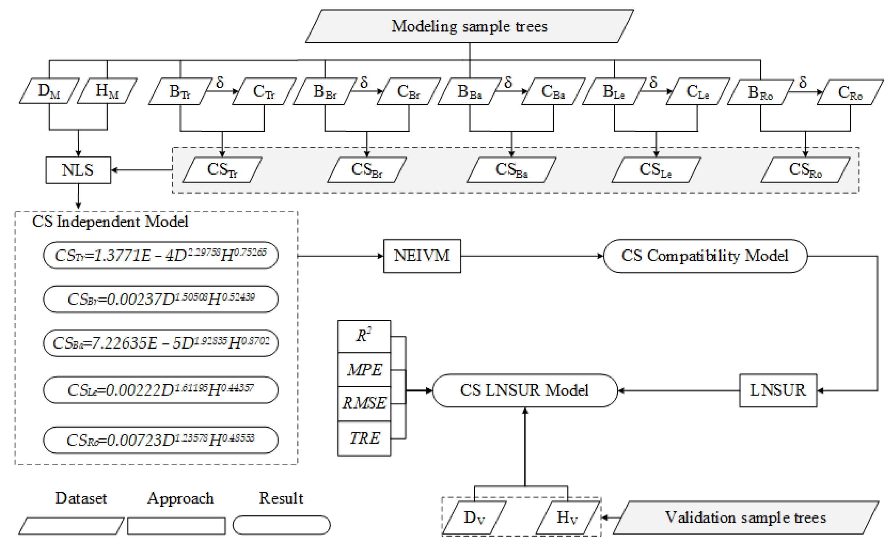
2.3. Construction of Olea europaea L. CS Model

2.3.1. CS Independent Model

The allometric growth equation demonstrates strong adaptability, high flexibility, and excellent fitting performance when constructing independent models for CS [16]. Considering that the growth habit of Olea europaea L. is similar to that of acacia and oak plantations, and that it can adapt to environments such as drought and poor soils [27], we referred to similar modeling methods and screened D, H, and D-H composite factors (DH, D²H, D^bH^c) based on the results of Pearson correlation analysis, and constructed an independent model of Olea europaea L. CS by using Origin 2021 software (The Olea europaea L. CS, D, and H data were initially imported into the worksheet. Nonlinear curve fitting was then performed through the menu path “Analysis → Fitting → Nonlinear Curve Fit”. A power function model was selected from the built-in function library to establish the mathematical relationship between variables. The fitting procedure automatically calculated the model parameters (a, b, and c). The data for the selected sample trees D and H were evenly distributed; 96 sample trees were selected to construct the model according to the typical sampling method, and the remaining 24 sample trees were used as test data for the generalization test of the model. The nonlinear regression method was used, and the power function model was selected as the base function model to fit the univariate and binary independent model of Olea europaea L. CS with the measured Olea europaea L. CS as the dependent variable, and the readily measurable factors D, DH, D²H, and D^bH^c as the independent variables. The formulas are as follows:

$$\left\{\begin{array}{l}C=a{D}^b\\ C=a{\left(\mathit{DH}\right)}^b\\ C=a{\left(D^{2}H\right)}^b\\ C=a{D}^b{H}^c\end{array}\right.$$

(1)

where C is the CS of each organ (kg); D is the ground diameter (cm); H is the height of the tree (cm); a, b, and c are model parameters.

2.3.2. CS Compatibility Model

The CS independent model usually builds separate regression models for each organ CS and modeling factor, which may result in the total CS of the model not being equal to the sum of the components, i.e., the problem of model incompatibility occurs [28]. We have found that birch is drought-resistant, adapted to poor soils, and can improve soils, restore degraded ecosystems, and has a high economic value. Olea europaea L. has similar characteristics. Given that Robinia pseudoacacia and Betula platyphylla have been successfully modeled for biomass compatibility using nonlinear metric error models, a similar approach can be applied to Olea europaea L. [15,28]. In this study, we used PyCharm 2021.3 software (with Python 3.9 as the interpreter). Initially, a basic nonlinear model and the corresponding initial parameters were defined. Subsequently, a target function (the nonlinear_model function) was constructed to calculate the difference between the model’s predicted values and the actual observed values, with these differences serving as the fitting objective. To optimize the model parameters, the scipy.optimize.least_squares function was employed, which minimizes the error between the predicted and observed values to solve for the optimal parameters. By modifying the form of the nonlinear_model function, it can accommodate different error distributions or measurement characteristics, thus enabling its application to the fitting of nonlinear error models). A nonlinear metric error model was employed to model CS compatibility and select the optimal model based on evaluation metrics. Nonlinear metric error models characterize the nonlinear relationship between measurements and errors. They provide more accurate estimates than traditional linear error models by better capturing the complexity of error characteristics as they vary with measurements, especially when the error exhibits a nonlinear distribution [29,30]. The standard form of the model is as follows:

$$\left\{\begin{array}{l}f\left(y_i,x_i,c\right)=0\\ Y_i=y_i+e_i,i=1,\dots ,n\\ E_{\left(e_i\right)}=0, \mathit{cov}\left(e_i\right)={\sigma }^2\phi \end{array}\right.$$

(2)

where x_i is the q-dimensional error-free observation, y_i is the observation of the p-dimensional error variable, the m-dimensional vector function at time f, and y_i is the to-be-estimated truth value of Y_i; the covariance matrix of the error e_i is denoted as φ = σ²Ψ, Ψ is the error structure matrix of e_i, which is known or unknown, and σ² is unknown.

$$\left\{\begin{array}{l}{C}_1=f_1\left(x_1\right)+{\epsilon }_1\\ C_2=f_2\left(x_2\right)+{\epsilon }_2\\ C_3=f_3\left(x_3\right)+{\epsilon }_3\\ C_4=f_4\left(x_4\right)+{\epsilon }_4\\ C=f_1\left(x_1\right)+f_2\left(x_2\right)+f_3\left(x_3\right)+f_4\left(x_4\right)+\epsilon \end{array}\right.$$

(3)

where C₁, C₂, C₃, C₄, and C are trunk, branches, bark, leaves CS, and AGCS (kg), respectively; f₁ (x₁), f₂ (x₂), f₃ (x₃), and f₄ (x₄) are trunk, branch, bark, leaves, and AGCS models, respectively; and ε₁, ε₂, ε₃, ε₄, and ε are the various random errors, respectively.

The optimal Olea europaea L. CS independent model was utilized to construct the Olea europaea L. CS compatibility model by dividing the AGCS model into four subcomponents: trunk, branches, bark, and leaves, ensuring that the sum of the subcomponents equals the total AGCS. The CS compatibility model was constructed by directly controlling and distributing the subcomponents within the AGCS framework.

(1)

Unitary compatibility model

$$\left\{\begin{array}{l}{C}_1=\left({\displaystyle \frac{a_1{D}^{b_1}}{a_1{D}^{b_1}+a_2{D}^{b_2}+a_3{D}^{b_3}+a_4{D}^{b_4}}}\right)\times a{D}^b\\ C_2=\left({\displaystyle \frac{a_2{D}^{b_2}}{a_1{D}^{b_1}+a_2{D}^{b_2}+a_3{D}^{b_3}+a_4{D}^{b_4}}}\right)\times a{D}^b\\ C_3=\left({\displaystyle \frac{a_3{D}^{b_3}}{a_1{D}^{b_1}+a_2{D}^{b_2}+a_3{D}^{b_3}+a_4{D}^{b_4}}}\right)\times a{D}^b\\ C_4=\left({\displaystyle \frac{a_4{D}^{b_4}}{a_1{D}^{b_1}+a_2{D}^{b_2}+a_3{D}^{b_3}+a_4{D}^{b_4}}}\right)\times a{D}^b\\ C=a{D}^b=C_1+C_2+C_3+C_4\end{array}\right.$$

(4)

Let r₁ = a₂/a₁, r₂ = a₃/a₁, r₃ = a₄/a₁, k₁ = b₂ − b₁, k₂ = b₃ − b₁, k₃ = b₄ − b₁ to obtain Equation (5). Where r₁~r₃, k₁~k₃, a, b, and c are the parameters to be estimated, and their initial values are the values of the parameters of the trunk, branch, bark, leaves, and the AGCS unitary independent model.

$$\left\{\begin{array}{c}{C}_1={\displaystyle \frac{a{D}^b}{1+r_1{D}^{k_1}+r_2{D}^{k_2}+r_3{D}^{k_3}}}\\ C_2={\displaystyle \frac{a{r}_1{D}^{\left(k_1+b\right)}}{1+r_1{D}^{k_1}+r_2{D}^{k_2}+r_3{D}^{k_3}}}\\ C_3={\displaystyle \frac{a{r}_2{D}^{\left(k_2+b\right)}}{1+r_1{D}^{k_1}+r_2{D}^{k_2}+r_3{D}^{k_3}}}\\ C_4={\displaystyle \frac{a{r}_3{D}^{\left(k_3+b\right)}}{1+r_1{D}^{k_1}+r_2{D}^{k_2}+r_3{D}^{k_3}}}\end{array}\right.$$

(5)

(2)

Binary compatibility model

$$\left\{\begin{array}{l}{C}_1=\left({\displaystyle \frac{a_1{D}^{b_1}{H}^{c_1}}{a_1{D}^{b_1}{H}^{c_1}+a_2{D}^{b_2}{H}^{c_2}+a_3{D}^{b_3}{H}^{c_3}+a_4{D}^{b_4}{H}^{c_4}}}\right)\times a{D}^b{H}^c\\ C_2=\left({\displaystyle \frac{a_2{D}^{b_2}{H}^{c_2}}{a_1{D}^{b_1}{H}^{c_1}+a_2{D}^{b_2}{H}^{c_2}+a_3{D}^{b_3}{H}^{c_3}+a_4{D}^{b_4}{H}^{c_4}}}\right)\times a{D}^b{H}^c\\ C_3=\left({\displaystyle \frac{a_3{D}^{b_3}{H}^{c_3}}{a_1{D}^{b_1}{H}^{c_1}+a_2{D}^{b_2}{H}^{c_2}+a_3{D}^{b_3}{H}^{c_3}+a_4{D}^{b_4}{H}^{c_4}}}\right)\times a{D}^b{H}^c\\ C_4=\left({\displaystyle \frac{a_4{D}^{b_4}{H}^{c_4}}{a_1{D}^{b_1}{H}^{c_1}+a_2{D}^{b_2}{H}^{c_2}+a_3{D}^{b_3}{H}^{c_3}+a_4{D}^{b_4}{H}^{c_4}}}\right)\times a{D}^b{H}^c\\ C=a{D}^b{H}^c=C_1+C_2+C_3+C_4\end{array}\right.$$

(6)

Let r₁ = a₂/a₁, r₂ = a₃/a₁, r₃ = a₄/a₁, k₁ = b₂ − b₁, k₂ = b₃ − b₁, k₃ = b₄ − b₁, f₁ = c₂ − c₁, f₂ = c₃ − c₁, f₃ = c₄ − c₁ to obtain Equation (7). Where r₁~r₃, k₁~k₃, f₁~f₃, a, b, and c are the parameters to be estimated, with their initial values derived from the parameters of the trunk, branches, bark, leaves, and the AGCS binary independent model.

$$\left\{\begin{array}{c}{C}_1={\displaystyle \frac{a{D}^b{H}^c}{1+r_1{D}^{k_1}{H}^{f_1}+r_2{D}^{k_2}{H}^{f_2}+r_3{D}^{k_3}{H}^{f_3}}}\\ C_2={\displaystyle \frac{r_{1}a{D}^{\left(k_1+b\right)}{H}^{\left(f_1+c\right)}}{1+r_1{D}^{k_1}{H}^{f_1}+r_2{D}^{k_2}{H}^{f_2}+r_3{D}^{k_3}{H}^{f_3}}}\\ C_3={\displaystyle \frac{r_{2}a{D}^{\left(k_2+b\right)}{H}^{\left(f_2+c\right)}}{1+r_1{D}^{k_1}{H}^{f_1}+r_2{D}^{k_2}{H}^{f_2}+r_3{D}^{k_3}{H}^{f_3}}}\\ C_4={\displaystyle \frac{r_{3}a{D}^{\left(k_3+b\right)}{H}^{\left(f_3+c\right)}}{1+r_1{D}^{k_1}{H}^{f_1}+r_2{D}^{k_2}{H}^{f_2}+r_3{D}^{k_3}{H}^{f_3}}}\end{array}\right.$$

(7)

2.3.3. LNSUR Model

The NSUR method is widely recognized as a reliable method when estimating parameters in compatible modeling systems [31], which ensures additivity among the components of the Olea europaea L. CS and reduces the confidence and prediction intervals of the CS [11]. The method not only takes into account the correlation between partial equations but also ensures compatibility between different models for efficient parameter estimation [13,32]. NSUR can be regarded as a nonlinear counterpart of Seemingly Uncorrelated Regression (SUR), which is a generalized linear model with a specific error structure matrix. The formula for the SUR model is as follows:

$$\left\{\begin{array}{l}y=x\beta +e\\ E\left(e\right)=0\\ \mathit{cov}\left(e\right)=\sum \otimes \mathit{Ln}\end{array}\right.$$

(8)

where x is the full-rank column matrix, β is the parameter vector, Σ is the error covariance matrix, e is the error vector, and Ln denotes the n × n unit matrix.

However, heteroscedasticity is a common issue when constructing CS models, characterized by unequal variances of the residuals. Addressing heteroscedasticity is crucial for accurately estimating the parameters of the NSUR model. Weighted regression is typically used to address heteroscedasticity, but in cases of small sample sizes, accurately determining the variance pattern of the error terms becomes challenging, and the weighted regression method may not effectively correct heteroscedasticity [33]. Therefore, in this study, the residual variance in the samples was estimated collectively using a logarithmic transformation method, which has been successfully applied in evergreen and deciduous plants such as Picea rubens, Pinus resinosa, and Larix decidua [34]. Given the similar ecological characteristics of Olea europaea L. and the fact that the logarithmic transformation can effectively eliminate the tendency of heteroskedasticity due to variation, thus stabilizing the variance and achieving homoskedasticity, the reliability of parameter estimation in the NSUR model is improved. This study utilized Stata software (version 17), and the model parameters were estimated using the NSUR method within this software. First, each nonlinear equation was defined separately using the “nl” command in Stata, followed by joint estimation using the NSUR method. During the estimation process, the “initial()” option was used to specify parameter starting values to ensure model convergence, and the “tolerance()” parameter was employed to adjust the convergence criteria for optimizing the estimation results. The logarithmic transformation process is as follows:

$$\mathit{Ln}\left(Y-\epsilon \right)=\mathit{Ln}\left[Y\left(1-\epsilon /Y\right)\right]=\mathit{LnY}+\mathit{Ln}\left(1-\epsilon /Y\right)=a+\mathit{bLnX}$$

(9)

Let ε/Y = k, considering that k is very small, Equation (10) is obtained by using a series expansion and keeping it only once:

$$\mathit{LnY}\approx a+\mathit{bLnX}+k$$

(10)

Independent models of Olea europaea L. CS with D and D²H as independent variables were coded separately (11), (12):

$$\left\{\begin{array}{l}\mathit{Ln}{C}_1\approx a_1+b_1\mathit{LnD}+k_1\\ \mathit{Ln}{C}_2\approx a_2+b_2\mathit{LnD}+k_2\\ \mathit{Ln}{C}_3\approx a_3+b_3\mathit{LnD}+k_3\\ \mathit{Ln}{C}_4\approx a_4+b_4\mathit{LnD}+k_4\\ \mathit{LnC}\approx \mathit{Ln}\left(e^{a_1}{D}^{b_1}+e^{a_2}{D}^{b_2}+e^{a_3}{D}^{b_3}+e^{a_4}{D}^{b_4}\right)+k_5\end{array}\right.$$

(11)

$$\left\{\begin{array}{l}\mathit{Ln}{C}_1\approx a_1+b_1\mathit{Ln}\left(D^{2}H\right)+k_1\\ \mathit{Ln}{C}_2\approx a_2+b_2\mathit{Ln}\left(D^{2}H\right)+k_2\\ \mathit{Ln}{C}_3\approx a_3+b_3\mathit{Ln}\left(D^{2}H\right)+k_3\\ \mathit{Ln}{C}_4\approx a_4+b_4\mathit{Ln}\left(D^{2}H\right)+k_4\\ \mathit{LnC}\approx \mathit{Ln}\left[e^{a_1}{\left(D^{2}H\right)}^{b_1}+e^{a_2}{\left(D^{2}H\right)}^{b_2}+e^{a_3}{\left(D^{2}H\right)}^{b_3}+e^{a_4}{\left(D^{2}H\right)}^{b_4}\right]+k_5\end{array}\right.$$

(12)

2.4. Model Accuracy Assessment

In this study, the samples were divided into modeling samples and testing samples according to the ratio of 8:2 to construct and test the model. Based on Excel 2016 software (Average Function, Sum Function, Absolute Value Function, Square Root Function), the model fitting accuracy was evaluated based on the coefficient of determination (R²), Mean Prediction Error (MPE, %), Root Mean Square Error (RMSE, kg), and Total Relative Error (TRE, %). These metrics have been well validated in CS modeling tests for pure Larix gmelinii (Rupr.) Kuzen. forests [7]:

$$\left\{\begin{array}{l}{R}^2=1-{\displaystyle \frac{{\sum }_{i=1}^n{\left(y_i-{\widehat{y}}_i\right)}^2}{{\sum }_{i=1}^n{\left(y_i-{\overline{y}}_i\right)}^2}}\\ MPE={\displaystyle \frac{100}{n}}{\displaystyle \sum _{i=1}^n}{\displaystyle \frac{\left|y_i-{\widehat{y}}_i\right|}{y_i}}\\ RMSE=\sqrt{{\displaystyle \frac{{\sum }_{i=1}^n{\left(y_i-{\widehat{y}}_i\right)}^2}{n-1}}}\\ TRE={\displaystyle \frac{{\sum }_{i=1}^n\left(y_i-{\widehat{y}}_i\right)}{{\sum }_{i=1}^n{\widehat{y}}_i}}\times 100\end{array}\right.$$

(13)

where $y_i$ is the measured value of CS for each organ, ${\widehat{y}}_i$ is the predicted value of CS for each organ, ${\overline{y}}_i$ is the mean value of CS for each organ, and n is the number of Olea europaea L. sample trees.

3. Results

3.1. Optimal CS Independent Model

The nonlinear CS estimation of each organ of Olea europaea L. was carried out, and the fitting quality was evaluated according to R², MPE, RMSE, and TRE (

Table 3. Statistical results of independent models and test indices for CS of each organ of Olea europaea L., constructed based on power function forms.

Organ	CS Model	Fitting Formula	R2	MPE	RMSE	TRE
Trunk	C = aDb	C = 0.00496D2.65726	0.905	26.532	0.945	0.914
	C = a(DH)b	C = 4.26305E − 6(DH)1.62211	0.895	23.738	0.996	−0.826
	C = a(D2H)b	C = 4.03036E − 5(D2H)1.04609	0.927	20.713	0.827	−0.013
	C = aDbHc	C = 1.3771E − 4D2.29758H0.75265	0.931	21.524	0.804	0.427
Branch	C = aDb	C = 0.02896D1.75331	0.709	29.981	0.730	0.919
	C = a(DH)b	C = 1.98879E − 4(DH)1.10686	0.703	27.785	0.738	0.096
	C = a(D2H)b	C = 0.00109(D2H)0.69899	0.724	27.418	0.711	0.469
	C = aDbHc	C = 0.00237D1.50508H0.52439	0.726	27.769	0.709	0.629
Bark	C = aDb	C = 0.00462D2.33944	0.715	35.324	0.667	1.334
	C = a(DH)b	C = 6.44296E − 6(DH)1.46964	0.731	33.358	0.648	−0.127
	C = a(D2H)b	C = 5.37873E − 5(D2H)0.94012	0.748	31.815	0.627	0.695
	C = aDbHc	C = 7.22635E − 5D1.92835H0.8702	0.749	31.932	0.627	0.806
Leaves	C = aDb	C = 0.01883D1.81405	0.715	35.849	0.569	0.642
	C = a(DH)b	C = 1.11394E − 4(DH)1.14226	0.696	35.672	0.587	−0.031
	C = a(D2H)b	C = 6.39547E − 4(D2H)0.72241	0.722	34.255	0.562	0.290
	C = aDbHc	C = 0.00222D1.61195H0.44357	0.726	34.344	0.557	0.492
Root (BGCS)	C = aDb	C = 0.07892D1.42825	0.671	27.897	0.766	0.042
	C = a(DH)b	C = 8.99959E − 4(DH)0.95572	0.669	30.014	0.768	−0.366
	C = a(D2H)b	C = 0.00444(D2H)0.59079	0.685	28.380	0.748	−0.106
	C = aDbHc	C = 0.00723D1.23578H0.48553	0.686	28.103	0.747	−0.053
AGCS	C = aDb	C = 0.03465D2.24598	0.884	21.499	2.175	1.182
	C = a(DH)b	C = 7.1117E − 5(DH)1.39622	0.878	20.770	2.235	−0.120
	C = a(D2H)b	C = 5.42937E − 4(D2H)0.89188	0.906	18.957	1.957	0.514
	C = aDbHc	C = 0.0014D1.92876H0.67174	0.909	19.164	1.929	0.793

). The optimal model is C = aD^bH^c. Among them, the optimal independent model for trunk CS was C = 1.3771E − 4D^2.29758H^0.75265, for branch CS was C = 0.00237D^1.50508H^0.52439, for bark CS was C = 7.22635E − 5D^1.92835H^0.8702, for leaf CS was C = 0.00222D^1.61195H^0.44357, for root CS (BGCS) was C = 0.00723D^1.23578H^0.48553, and for AGCS was C = 0.0014D^1.92876H^0.67174.

The generalizability of each optimal model was validated using testing samples. The evaluation metrics demonstrated robust model performance (

Table 4. Statistical results of metrics for generalizability testing of the optimal independent models for each organ screened using a 20% testing sample.

Organ	CS Model	Fitting Formula	R2	MPE	RMSE	TRE
Trunk	C = aDbHc	C = 1.3771E − 4D2.29758H0.75265	0.832	30.333	1.153	−0.434
Branch	C = aDbHc	C = 0.00237D1.50508H0.52439	0.721	25.923	0.716	9.886
Bark	C = aDbHc	C = 7.22635E − 5D1.92835H0.8702	0.722	24.456	0.508	3.856
Leaves	C = aDbHc	C = 0.00222D1.61195H0.44357	0.570	37.124	0.713	11.507
Root	C = aDbHc	C = 0.00723D1.23578H0.48553	0.736	27.563	0.735	−1.588
AGCS	C = aDbHc	C = 0.0014D1.92876H0.67174	0.871	20.018	2.073	5.074

), with the R² ranging from 0.570 to 0.871, MPE varied between 20.018% and 37.124%, while RMSE ranged from 0.508 kg to 2.073 kg. TRE ranged from −1.588% to 11.507%. These results indicate that the models provide reliable predictions and are suitable for estimating the whole-plant CS in Olea europaea L.

To further investigate the relationship between predicted and measured values for each model, scatter plots were generated comparing the predicted and measured CS values for each organ (Figure 4). Linear regression fitting (Y = kx + b) was applied, yielding R² ranging from 0.747 to 0.881, with slope values (k) between 0.716 and 0.940. These results demonstrate that the predicted values closely align with the measured values, indicating excellent model fit and high predictive accuracy.

3.2. CS Compatibility Model for Each Organ

The compatibility model employed a weighted regression approach to address heteroskedasticity, building upon the established independent models to develop univariate and binary compatibility models for Olea europaea L. CS. This weighted regression method effectively improved model heteroskedasticity (Figure 5 and Figure 6. Note: The red dotted line represents the reference line where the residuals are zero, and each point in blue represents a prediction. Blue dots randomly and uniformly distributed above and below the red dotted line, and close to it, indicate that the model has minimal bias), with parameter estimates for the compatibility model detailed in

Table 5. Parameter estimates for univariate and binary AGCS compatibility models.

	Model Type	Univariate	Binary
Parameters
a		0.0346691	0.0014155
b		2.2457308	1.9287284
c			0.6698741
r1		5.1440537	22.2450445
r2		0.9246553	0.5577064
r3		3.3038916	20.4319071
k1		−0.8565350	−0.7296256
k2		−0.3149435	−0.3426050
k3		−0.7913422	−0.6298362
f1			−0.2985259
f2			0.0956456
f3			−0.3730051

.

A comparison of evaluation metrics in

Table 6. Fit analysis of Olea europaea L. organs under univariate and binary compatibility models: comparative statistics based on R², MPE, RMSE, and TRE indicators.

Model Type	Organ	Testing Indicators
		R2	MPE	RMSE	TRE
Univariate	Trunk	0.905	−6.135	0.943	0.187
	Branch	0.706	−6.697	0.729	0.265
	Bark	0.714	−13.064	0.665	0.289
	Leaves	0.713	−13.371	0.568	0.259
	AGCS	0.884	−3.004	2.164	0.172
Binary	Trunk	0.931	−4.438	0.800	0.162
	Branch	0.724	−6.437	0.707	0.254
	Bark	0.747	−10.554	0.625	0.276
	Leaves	0.725	−13.543	0.556	0.251
	AGCS	0.909	−2.195	1.918	0.159

revealed that the binary model outperformed the univariate model in terms of prediction accuracy and goodness of fit across multiple organs. Specifically, the binary model exhibited higher R², particularly for trunk (0.931 vs. 0.905) and AGCS (0.909 vs. 0.884), indicating a superior fit for these components. Additionally, the binary model demonstrated lower MPE, with reduced errors for trunk (−4.438 vs. −6.135) and AGCS (−10.39 vs. −13.66), suggesting less bias and greater accuracy. In terms of RMSE, the binary model consistently achieved lower errors, notably for the trunk (0.800 vs. 0.943) and other organs such as branches, bark, and leaves, highlighting its enhanced precision. Furthermore, the binary model exhibited smaller TRE values, such as for the trunk (0.162 vs. 0.187), further validating its reliability.

In summary, the binary model demonstrated superior fit, reduced prediction errors, and stronger predictive capability for organs, including trunk, branch, bark, leaves, and AGCS, highlighting its effectiveness and superiority in this study.

3.3. CS LNSUR Model

In this study, D and D²H were used as independent variables, respectively, and the estimated parameters and fit indices of the additivity CS equation are shown in

Table 7. Parameters and test metric results of the improved CS compatibility model using the LNSUR method with selected variable factors D and D²H.

Variable	Organ	a	b	R2	MPE	RMSE	TRE
D	Trunk	−4.9551	2.4977	0.873	−26.185	0.335	28.930
	Branch	−3.2209	1.6165	0.733	−24.640	0.329	41.542
	Bark	−5.0375	2.1723	0.801	672.234	0.380	836.374
	Leaves	−3.9243	1.7870	0.693	−74.706	0.418	120.344
	Root	−2.8500	1.5258	0.766	8.334	0.307	36.141
	AGCS	−2.8883	2.0493	0.866	−37.829	0.283	11.423
D2H	Trunk	−10.0297	1.0343	0.910	−9.773	0.281	23.750
	Branch	−6.5314	0.6719	0.770	74.271	0.318	46.524
	Bark	−9.4859	0.9029	0.841	362.885	0.339	751.624
	Leaves	−7.5306	0.7377	0.718	−70.617	0.400	114.479
	Root	−6.2625	0.6629	0.787	2.701	0.293	35.303
	AGCS	−7.0525	0.8487	0.903	−18.167	0.241	9.867

. In terms of model fitting, the RMSE values were significantly lower than the CS weights shown in Table 1, which indicates that the LNSUR method can accurately estimate Olea europaea L. CS. Additionally, the LNSUR model produced smaller RMSE values for each sub-component of the CS compared to the traditional CS independent model. When D was the only independent variable in the set of equations, the R² of the LNSUR model was higher than 0.700 except for the leaves, and the trunk R² was the highest at 0.873, which is in line with the distribution of CS in the whole Olea europaea L. Compared to using D as a single independent variable, the total CS of Olea europaea L. estimated using the combined variables D²H showed higher precision, with the lowest R² of 0.718 for leaves and the highest R² of 0.910 for the trunk. The LNSUR model demonstrated better estimation performance compared to the traditional CS independent model, with higher precision and improved estimation accuracy.

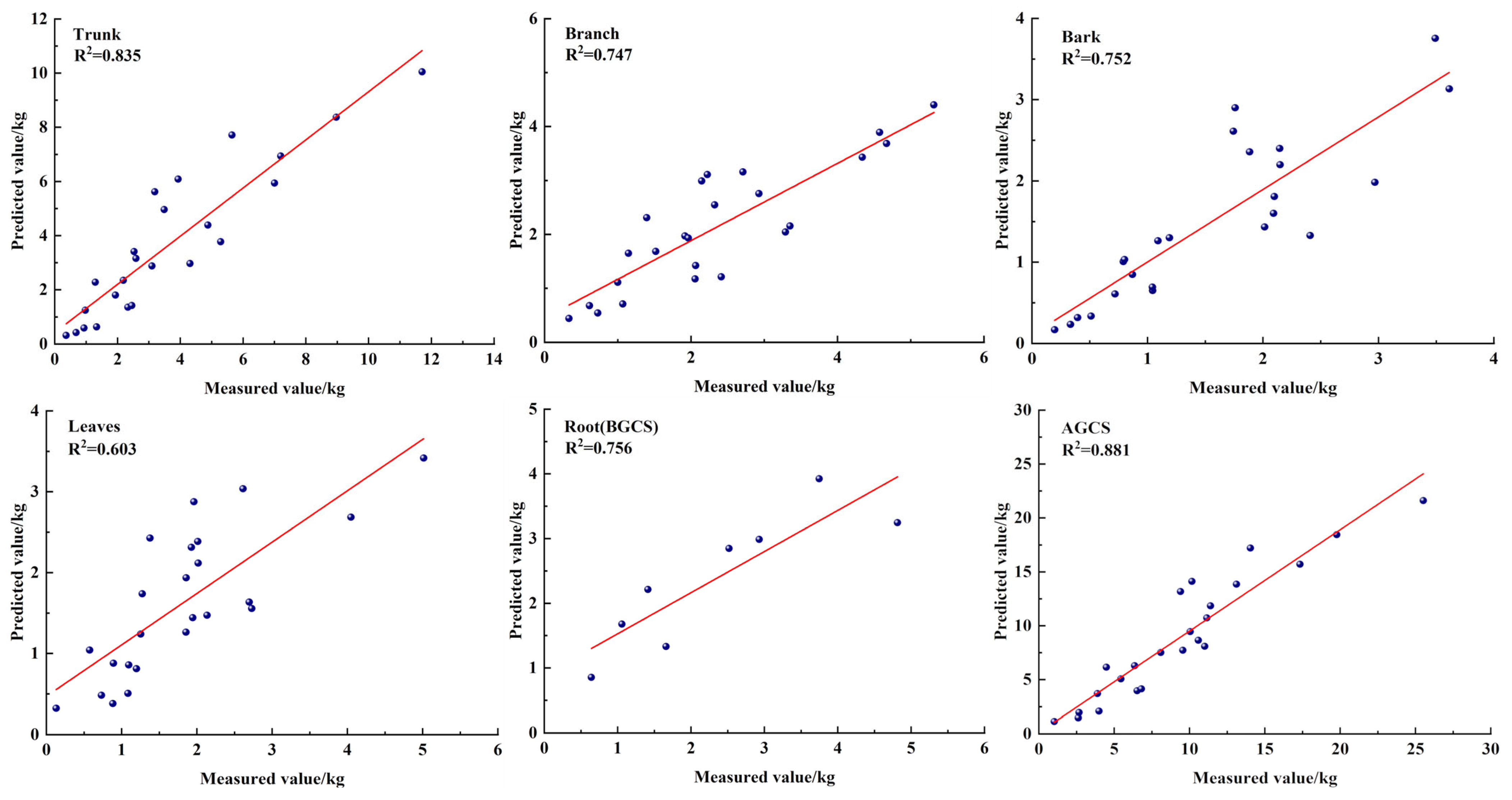
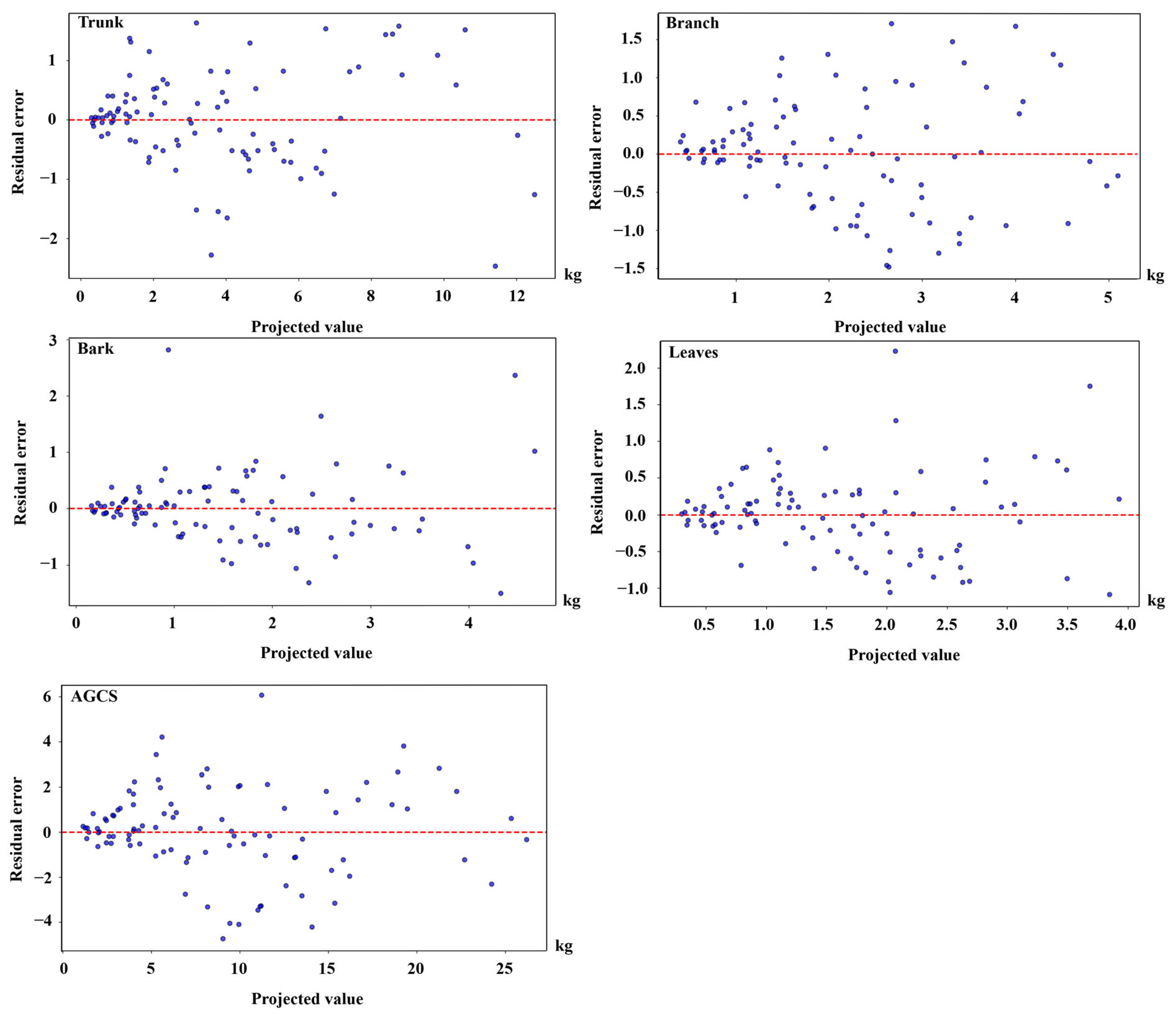
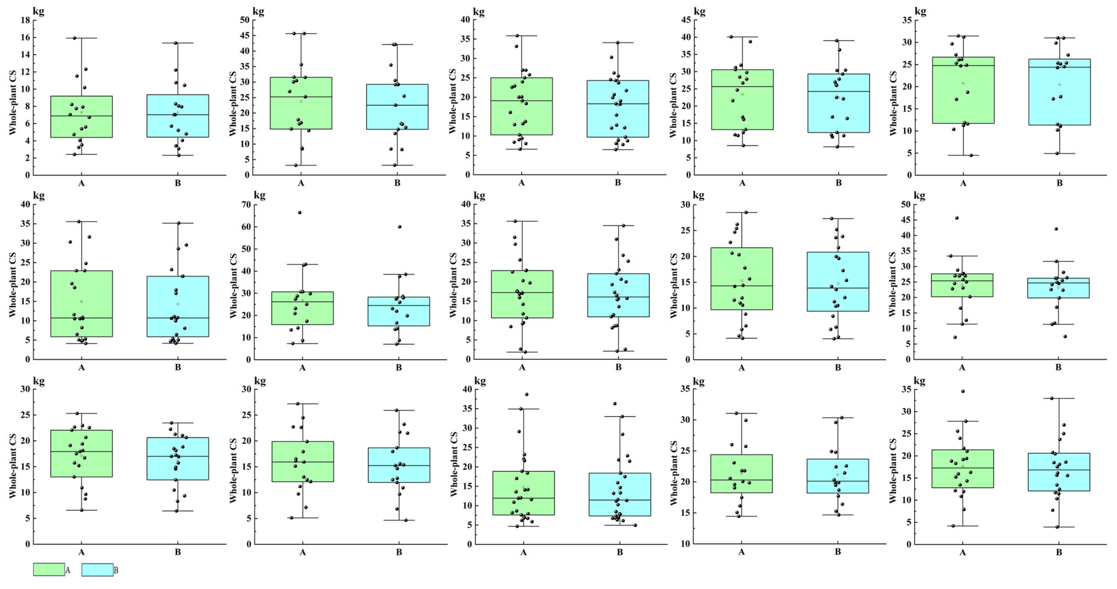
3.4. Estimation of Whole-Plant CS in Olea europaea L. from Validation Sample Trees

To further investigate the fitting accuracy and generalizability of the models, this study utilized the measured D and H data of a total of 284 Olea europaea L. trees in 15 sample plots to estimate the total CS of Olea europaea L. in each sample plot based on the CS independent model and the LNSUR model, respectively, as shown in Figure 7. The results showed that the CS independent model estimated the CS of 5221.863 kg, 0.696 kg per square meter, the LNSUR model estimated the CS of 5020.304 kg, 0.669 kg per square meter, and the R² was 0.964, MPE was 3.652, RMSE was 15.273, and TRE was 0.039, indicating that both the CS independent model and the LNSUR model exhibit high accuracy and are suitable for estimating the total CS of Olea europaea L. plants. Additionally, this study employed a t-test to evaluate the differences between the predicted values of the independent model and the LNSUR model. The test results indicated that there was no significant difference in mean levels between the two models, and the mean difference did not reach statistical significance. This suggests that the prediction results of the independent model and the LNSUR model are highly consistent, with both models demonstrating satisfactory predictive performance (

Table 8. T-test for whole-plant CS estimated by the independent CS model and the LNSUR model for 15 Olea europaea L. plots in the validation sample area.

	Index	T	p		Index	T	p
SN				SN
1		−0.800	0.436	9		5.114	0.000 *
2		4.793	0.083	10		2.024	0.052
3		5.648	0.000 *	11		2.367	0.099
4		3.614	0.006	12		3.752	0.002
5		1.615	0.127	13		1.743	0.094
6		3.871	0.000 *	14		−0.206	0.839
7		3.864	0.007	15		1.803	0.087
8		4.413	0.000 *

Note: 0.000 * means p < 10⁻⁴. When p ≥ 0.05, it means that the difference is not significant, and the model estimation is accurate.

).

4. Discussion

4.1. The First Attempt to Construct a CS Independent Model of Olea europaea L.

This study showed that an independent model of Olea europaea L. CS could be successfully constructed using the nonlinear least squares method, with measured Olea europaea L. CS data as the dependent variable and D and H as the independent variables (R² = 909 for the AGCS model and R² = 686 for the BGCS model). Among these, the trunk CS models exhibited high estimation accuracy (all R² > 0.900), similar to natural Larix gmelinii forests (R² = 0.959) [35], the trunk as the main part of the whole-plant CS of Olea europaea L., is easier to collect during field operations, and the sample collection is more complete. This is the primary reason for the higher accuracy of the trunk CS model. During the field collection of all organs, tree roots were the most challenging to collect due to their longer main roots and numerous lateral roots, making it difficult to collect them entirely. Although the same cross-section method was used in this study to replace some of the roots that were difficult to collect [24], the fitting accuracy of the CS model for tree roots was still relatively low but slightly higher than that of Ardisia japonica (Thunb.) Blume (R² = 0.600) [36], and Spatholobus suberectus Dunn (R² = 0.636) [10]. The generality test of the model revealed that the accuracy for tree leaves was the lowest (R² = 0.570), similar to that of the related species Pinus massoniana Lamb. (R² = 0.547) [37]. The main reason is that, as the primary photosynthetic organ of Olea europaea L., leaf CS is influenced by various environmental and physiological factors (e.g., light, temperature, humidity, soil nutrients, etc.). Additionally, the growth and distribution of leaves are more susceptible to seasonal variations, climatic conditions, and other external factors compared to other organs, such as the trunk and roots. Leaves also exhibit a high degree of spatial heterogeneity, which the model fails to fully account for, resulting in a lower R². Screening revealed that the optimal independent model for each CS was C = aD^bH^c, similar to the shrub biomass model [38]. During modeling, while D contributes the most to CS among the many easily measurable factors, a single-parameter model may fail to account for cases where the same D value corresponds to different CS values [39]. Overly complex models are prone to overfitting, making the model excessively sensitive to the data and leading to multicollinearity issues [40]. Including multiple variable factors in the model increases the workload of data collection, and errors during data collection can negatively impact the accuracy of CS estimation. Therefore, in practical application, appropriate variable factors and function forms should be selected for model construction according to the differences between research objects.

4.2. Construction of the Compatibility Model Using the CS Independent Model

We used a nonlinear metric error model system of joint equations based on the Olea europaea L. CS independent model to effectively construct the CS compatibility model, and this method can effectively address the problem of model incompatibility [41,42], which establishes the mathematical connection between components through algebraic means. The allocation method is then used to divide the total amount into four subsections, i.e., the AGCS is divided into the trunk, branches, bark, and leaves, ensuring that the sum of each subsection equals the total amount and resolving the incompatibility problem between the model’s components and the total amount. The AGCS is used to directly control and distribute the components to establish a compatible CS model. Addressing heteroskedasticity is particularly important when constructing the CS model. Many studies have used a weighting function approach to address heteroskedasticity [9].

This study shows that the fitting effect and prediction accuracy of the compatibility model of each organ are consistent with the independent model and exhibit smaller RMSE, which are consistent with the results of young trees in a typical plantation on the Qinghai–Tibet Plateau, China [43] and artificial Robinia pseudoacacia [39]. The R² of the univariate and binary compatibility models were above 0.700, and the prediction performance of the binary compatibility model was improved compared with the univariate compatibility model, which was similar to the results of the Eucalyptus globulus Labill and Artificial Young Forest in the Northwestern Alpine Region of China [44,45]. However, some studies have shown that the accuracy of the model decreases with the addition of tree H [46]. This may be related to the biological characteristics and habitats of the studied species, and H measurements are often challenging to obtain, especially for larger trees and those with overlapping canopies, leading to inaccuracies [47,48,49]. However, compatibility modeling ensures consistency between components, and studies have shown that compatibility models typically have smaller confidence intervals [50]. However, in practical applications, the applicability of the model and the challenges of obtaining relevant variable factors must be carefully considered.

4.3. Advantages of the LNSUR Model

In this study, the more accurately measured carbon coefficients were used to calculate the Olea europaea L. CS instead of using the commonly used international ratio of trees’ carbon content (0.45–0.50) [51]. The total carbon content of Olea europaea L. and the average carbon content of each organ (trunk, branches, bark, leaves, and roots) were 48.364%, 48.162%, 47.666%, 47.089%, 50.595%, and 48.309%, respectively. Using more accurate data sources, the accuracy of the Olea europaea L. CS compatibility model can be effectively improved through the LNSUR method. The LNSUR demonstrates significant advantages in the CS model. Theoretical analysis reveals that this method effectively eliminates cross-equation error correlations through the error covariance matrix and addresses heteroscedasticity using a weighting matrix [52]. Its inherent compatibility with logarithmically transformed allometric growth equations (e.g., W = aD^b) not only ensures valid parameter estimation but also strictly satisfies the additivity constraint [53]. The NSUR framework systematically addresses parameter bias from neglected error correlations in traditional NLS methods, achieving R² > 0.95 and MPE < 6% in Eucalyptus biomass modeling [54]. The results of this study showed that, compared with the independent model, the fitting results for the trunk, leaves, and AGCS did not change significantly, while the models for other organs showed substantial improvements. The tree root model exhibited the largest improvement (R² = 0.787), and the RMSE values were all reduced. The LNSUR binary model demonstrated better fitting performance, with results similar to those applied to Betula albo-sinensis Burk, Pinus armandii Franch, Pinus tabuliformis, and Quercus aliena var. acuteserrata, all of which achieved high accuracy in binary models with R² of 0.9572, 0.9754, 0.9651, and 0.9607 [13]. These findings support the reliability of constructing NSUR models using the logarithmic transformation method. The study emphasizes the effectiveness of the logarithmic transformation method in an additive modeling system [53], and the use of the LNSUR method for estimating parameters in the additive CS equations addresses the challenges of accurately capturing the underlying patterns of residual variation in the CS components [55]. However, current research on Olea europaea L. has primarily focused on breeding and cultivation, industrial development [56,57], disease control [58,59,60], and chemical composition [61,62], while research on Olea europaea L. CS has not been reported. The LNSUR method can not only effectively improve the accuracy of Olea europaea L. CS estimation and play a significant role in carbon sink management within agroforestry but also serve as a technical reference for CS estimation of other agroforestry crops. This further expands its application scope and enhances the overall benefits of carbon sinks.

5. Conclusions

In this study, the first attempt was made to construct a model for estimating the whole-plant CS of Olea europaea L. The following main conclusions were drawn: (1) The optimal independent model of Olea europaea L. AGCS was C = 0.0014D^1.92876H^0.67174 (R² = 0.909), and the BGCS model was C = 0.00723D^1.23578H^0.48553 (R² = 0.686). The AGCS compatibility model effectively addresses the issue of the sum of components not equaling the total, with a smaller RMSE. All constructed models exhibit high accuracy; (2) The LNSUR model showed a more pronounced improvement in accuracy for the Olea europaea L. BGCS model (R² = 0.787), and the estimated whole-plant CS also had a smaller RMSE; (3) Whole-plant CS was estimated in 15 Olea europaea L. sample plots using the CS independent and LNSUR models, achieving an R² of 0.964. Based on the whole-plant CS estimation model of Olea europaea L. constructed in this study, it provides a scientific basis for monitoring economic and ecological value indicators, such as Olea europaea L. yield and its carbon sink capacity. However, the limited extent of the study area and the small number of sampling points may introduce errors in the inversion results. Additionally, field data measurement errors, modeling uncertainties, and sampling variability can affect the estimation accuracy. In the future, further model optimization should be explored to account for the effects of environmental factors, different varieties, geographical regions, and other variables on Olea europaea L. CS. In addition, CS management in Olea europaea L. plantations should pay more attention to the relationship between long-term carbon sink effects and climate change to further enhance the accuracy of CS estimation. Future efforts should focus on improving existing models to enhance their accuracy and reliability in practical applications, assessing the impacts of different plantation management practices on CS, and providing more accurate decision support for the sustainable management and optimization of CS in Olea europaea L. plantations.

References

1. Mansour, H.M.M.; Zeitoun, A.A.; Abd-Rabou, H.S.; El Enshasy, H.A.; Dailin, D.J.; Zeitoun, M.A.A.; El-Sohaimy, S.A. Antioxidant and Anti-Diabetic Properties of Olive (Olea europaea) Leaf Extracts: In Vitro and In Vivo Evaluation. Antioxidants 2023, 12, 1275. [Google Scholar] [CrossRef] [PubMed]
2. Bouarroudj, K.; Tamendjari, A.; Larbat, R. Quality, Composition and Antioxidant Activity of Algerian Wild Olive (Olea europaea L. subsp. Oleaster) Oil. Ind. Crops Prod. 2016, 83, 484–491. [Google Scholar] [CrossRef]
3. Mirón, I.J.; Linares, C.; Díaz, J. The Influence of Climate Change on Food Production and Food Safety. Environ. Res. 2023, 216, 114674. [Google Scholar] [CrossRef]
4. Ito, A.; Nishina, K.; Noda, H.M. Impacts of Future Climate Change on the Carbon Budget of Northern High-Latitude Terrestrial Ecosystems: An Analysis Using ISI-MIP Data. Polar Sci. 2016, 10, 346–355. [Google Scholar] [CrossRef]
5. Wu, G.; Huang, G.; Lin, S.; Huang, Z.; Cheng, H.; Su, Y. Changes in Soil Organic Carbon Stocks and Its Physical Fractions along an Elevation in a Subtropical Mountain Forest. J. Environ. Manag. 2024, 351, 119823. [Google Scholar] [CrossRef] [PubMed]
6. Chen, X.; Guo, Y.; Chen, Z.; Luo, X.; Wang, P.; Shi, M.; Wang, X. A New Method for Estimating Forest Stand Carbon Stock: Segmentation and Modeling Based on Forest Aboveground Imagery. Ecol. Indic. 2024, 167, 112697. [Google Scholar] [CrossRef]
7. Lei, L.; Chai, G.; Wang, Y.; Jia, X.; Yin, T.; Zhang, X. Estimating Individual Tree Above-Ground Biomass of Chinese Fir Plantation: Exploring the Combination of Multi-Dimensional Features from UAV Oblique Photos. Remote Sens. 2022, 14, 504. [Google Scholar] [CrossRef]
8. Lv, Z.; Duan, A. Biomass and Carbon Storage Model of Cunninghamia Lanceolata in Different Production Areas. Sci. Silvae Sin. 2024, 60, 1–11. [Google Scholar]
9. Chen, X.; Xie, D.; Zhang, Z.; Sharma, R.P.; Chen, Q.; Liu, Q.; Fu, L. Compatible Biomass Model with Measurement Error Using Airborne LiDAR Data. Remote Sens. 2023, 15, 3546. [Google Scholar] [CrossRef]
10. Qin, L.; Meng, S.; Zhou, G.; Liu, Q.; Xu, Z. Uncertainties in above Ground Tree Biomass Estimation. J. For. Res. 2021, 32, 1989–2000. [Google Scholar] [CrossRef]
11. Wang, D.; Zhang, Z.; Zhang, D.; Huang, X. Biomass Allometric Models for Larix Rupprechtii Based on Kosak’s Taper Curve Equations and Nonlinear Seemingly Unrelated Regression. Front. Plant Sci. 2023, 13, 1056837. [Google Scholar] [CrossRef] [PubMed]
12. Sandoval, S.; Montes, C.R.; Olmedo, G.F.; Acuña, E.; Mena-Quijada, P. Modelling Above-Ground Biomass of Pinus Radiata Trees with Explicit Multivariate Uncertainty. For. Int. J. For. Res. 2022, 95, 380–390. [Google Scholar]
13. Xiong, N.; Qiao, Y.; Ren, H.; Zhang, L.; Chen, R.; Wang, J. Comparison of Parameter Estimation Methods Based on Two Additive Biomass Models with Small Samples. Forests 2023, 14, 1655. [Google Scholar] [CrossRef]
14. Parresol, B.R. Additivity of Nonlinear Biomass Equations. Can. J. For. Res. 2001, 31, 865–878. [Google Scholar] [CrossRef]
15. Wen, J.; Zhang, C.; Mu, L.; Zhao, Z.; Ma, H. Robinia Pseudoacacia Biomass Model in Coastal Area of Qinhuangdao City. J. Northwest For. Univ. 2024, 1–10. [Google Scholar]
16. Zeng, W.; Tang, S. Using Measurement Error Modeling Method to Establish Compatible Single-Tree Biomass Equations System. For. Res. 2010, 23, 797–803. [Google Scholar]
17. Cao, L.; Li, H. Comparison of Two Compatible Biomass Models: A Case Study from Three Broadleaved Tree Species in Guangdong. Chin. J. Ecol. 2019, 38, 1916–1925. [Google Scholar]
18. Zhao, D.; Westfall, J.; Coulston, J.W.; Lynch, T.B.; Bullock, B.P.; Montes, C.R. Additive Biomass Equations for Slash Pine Trees: Comparing Three Modeling Approaches. Can. J. For. Res. 2019, 49, 27–40. [Google Scholar] [CrossRef]
19. Cao, Q.V. A Unified System for Tree- and Stand-Level Predictions. For. Ecol. Manag. 2021, 481, 118713. [Google Scholar] [CrossRef]
20. Dong, L.; Zhang, L.; Li, F. Developing Additive Systems of Biomass Equations for Nine Hardwood Species in Northeast China. Trees 2015, 29, 1149–1163. [Google Scholar] [CrossRef]
21. Fu, L.; Lei, Y.; Wang, G.; Bi, H.; Tang, S.; Song, X. Comparison of Seemingly Unrelated Regressions with Error-in-Variable Models for Developing a System of Nonlinear Additive Biomass Equations. Trees 2016, 30, 839–857. [Google Scholar] [CrossRef]
22. Ning, D.; Lu, B.; Du, C.; Li, Y.; Liao, Y.; Zhang, Y. Division of Suitable Cultivation Areas for Olive in Yunnan Province. China For. Sci. Technol. 2008, 5, 39–41. [Google Scholar]
23. LY/T 2259-2014; Technical Regulation on Sample Collections for Biomass Modeling. National Forestry and Grassland Administration: Beijing, China, 2014.
24. Xu, H.; Wang, Z.; Li, Y.; He, J.; Wu, X. Dynamic Growth Models for Caragana korshinskii Shrub Biomass in China. J. Environ. Manag. 2020, 269, 110675. [Google Scholar] [CrossRef]
25. Zhu, B.; Yuan, J. Pressure Transfer Modeling for an Urban Water Supply System Based on Pearson Correlation Analysis. J. Hydroinform. 2014, 17, 90–98. [Google Scholar] [CrossRef]
26. Månsson, R.; Tsapogas, P.; Åkerlund, M.; Lagergren, A.; Gisler, R.; Sigvardsson, M. Pearson Correlation Analysis of Microarray Data Allows for the Identification of Genetic Targets for Early B-Cell Factor * [Boxs]. J. Biol. Chem. 2004, 279, 17905–17913. [Google Scholar] [CrossRef]
27. Blujdea, V.N.B.; Pilli, R.; Dutca, I.; Ciuvat, L.; Abrudan, I.V. Allometric Biomass Equations for Young Broadleaved Trees in Plantations in Romania. For. Ecol. Manag. 2012, 264, 172–184. [Google Scholar] [CrossRef]
28. Wang, W.; Wang, B.; Zhang, X.; Zhang, Q.; Hao, S. Biomass Estimation Models of Natural Betula Platyphylla Forests in Daxing’anling, Inner Mongolia. J. Northwest For. Univ. 2023, 38, 180–188. [Google Scholar]
29. Zeng, W.; Xia, Z.; Zhu, S.; Luo, H. Compatible Tree Volume and Above-Ground Biomass Equations for Chinese Fir Plantations in Guizhou. J. Beijing For. Univ. 2011, 33, 1–6. [Google Scholar]
30. Tang, S.; Li, Y.; Wang, Y. Simultaneous Equations, Error-in-Variable Models, and Model Integration in Systems Ecology. Ecol. Model. 2001, 142, 285–294. [Google Scholar] [CrossRef]
31. Trautenmüller, J.W.; Péllico Netto, S.; Balbinot, R.; Watzlawick, L.F.; Dalla Corte, A.P.; Sanquetta, C.R.; Behling, A. Regression Estimators for Aboveground Biomass and Its Constituent Parts of Trees in Native Southern Brazilian Forests. Ecol. Indic. 2021, 130, 108025. [Google Scholar] [CrossRef]
32. Zhou, Z.; Fu, L.; Zhou, C.; Sharma, R.P.; Zhang, H. Simultaneous Compatible System of Models of Height, Crown Length, and Height to Crown Base for Natural Secondary Forests of Northeast China. Forests 2022, 13, 148. [Google Scholar] [CrossRef]
33. Wang, J.H.; Li, F.R.; Dong, L.H. Additive Aboveground Biomass Equations Based on Different Predictors for Natural Tilia Linn. Ying Yong Sheng Tai Xue Bao 2018, 29, 3685–3695. [Google Scholar] [PubMed]
34. Dong, L.; Zhang, L.; Li, F. A Compatible System of Biomass Equations for Three Conifer Species in Northeast, China. For. Ecol. Manag. 2014, 329, 306–317. [Google Scholar] [CrossRef]
35. Wang, Y.; Dong, L.; Shi, J. Effect of Competition on the Prediction Accuracy of Individual Tree Biomass Model for Natural Larix Gmelinii Forests. Chin. J. Appl. Ecol. 2024, 35, 1474–1482. [Google Scholar]
36. Xia, Z.; Jia, B.; Wang, X.; Liu, J. Shrub Biomass Models of Castanopsis Kawakamii Natural Forest. J. Northwest For. Univ. 2024, 39, 30–38. [Google Scholar]
37. Qin, J.; Li, Y.; Ma, J.; Lan, C.; Li, H.; Tang, S.; Li, M. Biomass Model Construction and Distribution Pattern of Pinus Massoniana Plantations under Different Climatic Conditions in Guangxi. Guangxi Sci. 2020, 27, 165–174. [Google Scholar]
38. Liu, C.; Luo, D. Model Construction and Optimization of Abies Fabri Scrub Biomass in the Sedera Mountains. J. Green Sci. Technol. 2024, 26, 44–50. [Google Scholar]
39. Li, F.; Feng, Y.; Zhao, Y.; Zhu, J.; Wei, X.; Liang, W. Construction and Comparison of Artificial Robinia Pseudoacacia Biomass Model in Caijiachuan Watershed. J. For. Environ. 2024, 44, 62–70. [Google Scholar]
40. Sileshi, G.W. A Critical Review of Forest Biomass Estimation Models, Common Mistakes and Corrective Measures. For. Ecol. Manag. 2014, 329, 237–254. [Google Scholar] [CrossRef]
41. Peng, J.; Wang, Z.; Zhang, Y.; Liu, H.; Gu, G.; Peng, X.; Wu, J.; Ye, Z.; Zhang, S.; Shang, S. Construction of Compatible Individual Tree Biomass Model of Myrica Rubra Plantation. J. Zhejiang A&F Univ. 2022, 39, 272–279. [Google Scholar]
42. Cao, L.; Li, H. Establishment and Analysis of Compatible Biomass Model for Cinnamomum Camphora in Guangdong Province. J. For. Environ. 2018, 38, 458–465. [Google Scholar]
43. Zheng, X.; Yi, L.; Li, Q.; Bao, A.; Wang, Z.; Xu, W. Developing Biomass Estimation Models of Young Trees in Typical Plantation on the Qinghai-Tibet Plateau, China. Chin. J. Appl. Ecol. 2022, 33, 2923–2935. [Google Scholar]
44. Mao, C.; Yi, L.; Xu, W.; Dai, L.; Bao, A.; Wang, Z.; Zheng, X. Study on Biomass Models of Artificial Young Forest in the Northwestern Alpine Region of China. Forests 2022, 13, 1828. [Google Scholar] [CrossRef]
45. António, N.; Tomé, M.; Tomé, J.; Soares, P.; Fontes, L. Effect of Tree, Stand, and Site Variables on the Allometry of Eucalyptus Globulus Tree Biomass. Can. J. For. Res. 2007, 37, 895–906. [Google Scholar] [CrossRef]
46. Meng, S.; Liu, Q.; Zhou, G.; Jia, Q.; Zhuang, H.; Zhou, H. Aboveground Tree Additive Biomass Equations for Two Dominant Deciduous Tree Species in Daxing’anling, Northernmost China. J. For. Res. 2017, 22, 233–240. [Google Scholar] [CrossRef]
47. Kaushal, R.; Islam, S.; Tewari, S.; Tomar, J.M.S.; Thapliyal, S.; Madhu, M.; Trinh, T.L.; Singh, T.; Singh, A.; Durai, J. An Allometric Model-Based Approach for Estimating Biomass in Seven Indian Bamboo Species in Western Himalayan Foothills, India. Sci. Rep. 2022, 12, 7527. [Google Scholar] [CrossRef]
48. Hunter, M.O.; Keller, M.; Victoria, D.; Morton, D.C. Tree Height and Tropical Forest Biomass Estimation. Biogeosciences 2013, 10, 8385–8399. [Google Scholar] [CrossRef]
49. Chave, J.; Andalo, C.; Brown, S.; Cairns, M.A.; Chambers, J.Q.; Eamus, D.; Fölster, H.; Fromard, F.; Higuchi, N.; Kira, T.; et al. Tree Allometry and Improved Estimation of Carbon Stocks and Balance in Tropical Forests. Oecologia 2005, 145, 87–99. [Google Scholar] [CrossRef]
50. Wang, X.; Zhao, D.; Liu, G.; Yang, C.; Teskey, R.O. Additive Tree Biomass Equations for Betula Platyphylla Suk. Plantations in Northeast China. Ann. For. Sci. 2018, 75, 60. [Google Scholar] [CrossRef]
51. Fang, J.; Chen, A. Dynamic of forest biomass carbon pools in China and their significance. Acta Bot. Sin. 2001, 43, 967–973. [Google Scholar]
52. Vonderach, C.; Kändler, G.; Dormann, C.F. Consistent Set of Additive Biomass Functions for Eight Tree Species in Germany Fit by Nonlinear Seemingly Unrelated Regression. Ann. For. Sci. 2018, 75, 49. [Google Scholar] [CrossRef]
53. Bi, H.; Turner, J.; Lambert, M.J. Additive Biomass Equations for Native Eucalypt Forest Trees of Temperate Australia. Trees 2004, 18, 467–479. [Google Scholar] [CrossRef]
54. Cai, H.; Lu, F.; Xu, Z.; Pan, H.; Meng, X.; Zeng, W. Research and Development of Compatible and Additive Individual Tree Biomass Model Systems for Eucalyptus. For. Resour. Manag. 2023, 01, 87–93. [Google Scholar]
55. Laskar, S.Y.; Sileshi, G.W.; Nath, A.J.; Das, A.K. Allometric Models for above and Below-Ground Biomass of Wild Musa Stands in Tropical Semi Evergreen Forests. Glob. Ecol. Conserv. 2020, 24, 01208. [Google Scholar] [CrossRef]
56. De La Casa, J.A.; Bueno, J.S.; Castro, E. Recycling of Residues from the Olive Cultivation and Olive Oil Production Process for Manufacturing of Ceramic Materials. A Comprehensive Review. J. Clean. Prod. 2021, 296, 126436. [Google Scholar] [CrossRef]
57. Wang, R.; Zheng, J.; Huang, Y.; Jiang, D. Research Advances on Breeding and Cultivation Techniques of Olive. Biot. Resour. 2024, 46, 103–111. [Google Scholar]
58. Lantero, E.; Matallanas, B.; Callejas, C. Current Status of the Main Olive Pests: Useful Integrated Pest Management Strategies and Genetic Tools. Appl. Sci. 2023, 13, 12078. [Google Scholar] [CrossRef]
59. Ali, A.O.; Awla, H.K.; Rashid, T.S. Investigating the in Vivo Biocontrol and Growth-Promoting Efficacy of Bacillus sp. and Pseudomonas fluorescens against Olive Knot Disease. Microb. Pathog. 2024, 191, 106645. [Google Scholar] [CrossRef]
60. Montilon, V.; Potere, O.; Susca, L.; Bottalico, G. Phytosanitary Rules for the Movement of Olive (Olea europaea L.) Propagation Material into the European Union (EU). Plants 2023, 12, 699. [Google Scholar] [CrossRef] [PubMed]
61. Pennisi, R.; Ben Amor, I.; Gargouri, B.; Attia, H.; Zaabi, R.; Chira, A.B.; Saoudi, M.; Piperno, A.; Trischitta, P.; Tamburello, M.P.; et al. Analysis of Antioxidant and Antiviral Effects of Olive (Olea europaea L.) Leaf Extracts and Pure Compound Using Cancer Cell Model. Biomolecules 2023, 13, 238. [Google Scholar] [CrossRef] [PubMed]
62. Bencresciuto, G.F.; Mandalà, C.; Migliori, C.A.; Cortellino, G.; Vanoli, M.; Bardi, L. Assessment of Starters of Lactic Acid Bacteria and Killer Yeasts: Selected Strains in Lab-Scale Fermentations of Table Olives (Olea europaea L.) Cv. Leccino. Fermentation 2023, 9, 182. [Google Scholar] [CrossRef]
Figure 1. Technical roadmap for the construction and validation of CS models for Olea europaea L. (Note: DM, HM, DV, and HV represent the ground diameter and tree height of the modeling sample trees and validation sample trees, respectively; BTr, BBr, BBa, BLe, and BRo represent the biomass of the trunk, branches, bark, leaves, and roots, respectively; CTr, CBr, CBa, CLe, and CRo represent the carbon content coefficients of the trunk, branches, bark, leaves, and roots, respectively; CSTr, CSBr, CSBa, CSLe, and CSRo represent the carbon stock of the trunk, branches, bark, leaves, and roots, respectively; NLS: Nonlinear Least Squares; NEIVM: Nonlinear Errors-in-Variables Model; LNSUR: Logarithmic Nonlinear Seemingly Unrelated Regression; δ represents the Dry Combustion Method).
Agronomy 15 00917 g001
Figure 2. Geographic overview of the study area and the distribution of sampling sites. ((a) represents a digital elevation map of Eshan County, Yuxi City, Yunnan Province, China, and (b) represents an orthophoto of the study area taken aerially by a drone).
Agronomy 15 00917 g002
Figure 3. Sampling and processing flow for each organ of Olea europaea L.: from field collection to laboratory analysis.
Agronomy 15 00917 g003
Figure 4. Scatter plot of measured value and predicted value for the optimal models of different organs. (The red line represents the best-fit line, and the blue dots denote the measured values. The closer and more tightly clustered the blue dots are to the red line, the higher the accuracy of the model).
Agronomy 15 00917 g004
Figure 5. Plot analyzing the relationship between predicted values and residual errors (addressing heteroscedasticity) for each organ of Olea europaea L. when constructing the univariate compatibility models.
Agronomy 15 00917 g005
Figure 6. Plot analyzing the relationship between predicted values and residual errors (addressing heteroscedasticity) for each organ of Olea europaea L. when constructing the binary compatibility models.
Agronomy 15 00917 g006
Figure 7. Comparison of whole-plant CS in 15 Olea europaea L. sample plots estimated using the two models (A: estimates based on the CS independent model; B: estimates based on the LNSUR model).
Agronomy 15 00917 g007