Monitoring the Progression of Downy Mildew on Vineyards Using Multi-Temporal Unmanned Aerial Vehicle Multispectral Data

Abstract

Monitoring vineyard diseases such as downy mildew (Plasmopara viticola) is important for viticulture, enabling an early intervention and optimized disease management. This is crucial for disease monitoring, and the use of high-spatial-resolution multispectral data from unmanned aerial vehicles (UAVs) can allow to for a better understanding of disease progression. This study explores the application of UAV-based multispectral data for monitoring downy mildew infection in vineyards through multi-temporal analysis. This study was conducted in a vineyard plot in the Vinho Verde region (Portugal), where 84 grapevines were monitored, half of which received phytosanitary treatments while the other half were left untreated in this way during the growing season. Seven UAV flights were performed across different phenological stages to assess the effects of infection using spectral bands, vegetation indices, and morphometric parameters. The results indicate that downy mildew affects canopy area, height, and volume, restricting the vegetative growth. Spectral analysis reveals that infected grapevines show increased reflectance in the visible and red-edge bands and a progressive decline in near-infrared (NIR) reflectance. Several vegetation indices demonstrated a suitable response to the infection, with some of them being capable of detecting early-stage symptoms, while vegetation indices using red edge and NIR allowed us to track disease progression. These results highlight the potential of UAV-based multi-temporal remote sensing as a tool for vineyard disease monitoring, supporting precision viticulture and the assessment of phytosanitary treatment effectiveness.

1. Introduction

Precision viticulture approaches have shown potential over the past decade, with innovative and straightforward application possibilities [1,2]. The development of new sensors and data-processing methodologies for vineyard monitoring is expected to increase in the coming years, contributing to better vineyard management and facilitating the acquisition of environmental and crop-related data [3]. The integration of digital technologies into modern viticulture can address the demand for a high-quality yield and wines while prioritizing consumer health and promoting environmentally sustainable practices with minimal impact on natural resources [4]. However, grapevine disease detection and monitoring remain a challenge due to the impact of diseases such as downy mildew (Plasmopara viticola) on yield and quality. Downy mildew is a fungal disease that causes crop losses and requires frequent phytosanitary treatments. Climate variability has further aggravated disease prevalence, making real-time monitoring critical for sustainable vineyard management. Traditional detection methods, such as field scouting and laboratory analysis, are time-consuming, labor-intensive, and may not detect early-stage infections before visible damage occurs. Consequently, there is an increasing need for rapid, non-destructive detection methods that enable early intervention and improved disease management throughout the growing season [5].

Remote sensing has emerged as an alternative for disease detection and monitoring [5], enabling timely and accurate monitoring of vineyard health status. Precision viticulture and precision agriculture approaches can make use of data from remote platforms, such as satellites, unmanned aerial vehicles (UAVs), and ground-based sensors to monitor spatial and temporal variability [6,7]. In this context, UAVs have become widely used for their efficiency in surveying large areas quickly and capturing data with a high spatial resolution at low flight heights [8] and from different payload sensors [5], such as thermal infrared (TIR) [9,10,11], multispectral [12,13], hyperspectral [14,15,16], LiDAR [17], and RGB [18], which provide several benefits for vineyard monitoring [19]. Data from these sensors enable the generation of point clouds, orthorectified raster products, and the calculation of vegetation indices (VIs) [20] for mapping the vineyard and assessing its conditions, analyzing geometric parameters [21], segmenting grapevine vegetation [22], assessing crop water status [11], monitoring grapevine vigor [23], and detecting disease symptoms and their incidence [12,24]. However, recent advances in hyperspectral remote sensing, such as the availability of data from hyperspectral satellites (e.g., PRISMA), have expanded the capabilities for monitoring plant stress and disease detection in agriculture [25,26]. These advancements can complement UAV-based multispectral studies by providing additional spectral details useful for calibrating and validating field-level observations.

UAV-based data were already used for monitoring different anomalies in crops such as wheat [27], tobacco [28], citrus [29], banana [30], olive [31], apple [32], chestnut [33], cabbage [34], sunflower [35], and watermelon [36], with multispectral sensors demonstrating the capacity to identify disease-induced spectral changes [37]. However, research on UAV-based disease detection and multi-temporal monitoring of disease progression analysis is not widely explored. Most studies focus on single-date UAV imagery for disease detection, providing only a static snapshot of the infection status [24,30]. While single-flight disease detection is feasible [38], capturing the temporal dynamics of disease progression, data collected over multiple periods are indispensable. Since downy mildew is a dynamic disease that evolves over time, continuous monitoring is required to track infection spread and assess the effectiveness of phytosanitary treatments. Multi-temporal analysis of UAV-based multispectral data has shown potential for early disease detection by capturing temporal variations in plant reflectance before visible symptoms appear [39,40]. Thus, multispectral, multi-temporal data acquired throughout the grapevine growing season may provide an overview of vineyard disease development [41], allowing for monitoring pathogen spread and its progression. Moreover, the integration of the Global Navigation Satellite System (GNSS) and real-time kinematic (RTK) technology ensures accurate georeferencing, improving the reliability of spatiotemporal analysis [42]. By analyzing temporal variations in plant reflectance, changes associated with infection can be identified [9]. Early detection is crucial for integrated disease management, enabling efficient interventions, reducing the indiscriminate use of agrochemicals, and promoting sustainable viticulture practices [43].

Advanced approaches, such as biosensors and spectral imaging techniques, are also being explored due to their ability to detect biotic stress in grapevines before visible symptoms develop [44]. Biosensors facilitate rapid, on-site analysis [45], while spectral imaging offers continuous, large-scale monitoring. However, these non-invasive techniques often require complex data interpretation and additional processing [46]. The combination of conventional techniques (cultivation techniques [47], polymerase chain reaction (PCR) [48], sequencing, and immunological techniques [49]) and advanced techniques could provide a comprehensive approach to pathogen detection in vineyards [5,50]. Among these tools, UAVs emerge due to their ability to acquire data in a simple, rapid, and cost-effective manner to survey entire vineyard plots compared to previous methods [51], improving operational efficiency and also the precision and quality of obtained data, making them useful for precision viticulture [23].

To address these gaps, in this study, multi-temporal UAV-based multispectral imaging is used to monitor downy mildew progression in vineyards. The analysis integrates five spectral bands, ten VIs, and geometric properties (height, canopy area, and projected volume) to evaluate the effectiveness of UAV-based remote sensing for early disease detection and to assess the impact of phytosanitary treatments on canopy development. By examining spectral and structural changes over different phenological stages, this study aims to identify suitable indicators for early disease detection and improve decision-making for phytosanitary treatment scheduling. This approach has the potential to improve the accuracy of disease detection and allow better decision support, including the scheduling of phytosanitary treatments and the assessment of the effectiveness of the implemented measures [43].

2. Materials and Methods

2.1. Study Area

This study was conducted throughout the 2023 grapevine growth campaign in 2.2 hectares of Vitis vinifera cv. Loureiro, planted in 2009, located in the demarcated region of Vinho Verde, Viana do Castelo, northwestern Portugal (41°47′34.2″ N, 8°32′20.6″ W, 50 m altitude), as presented in Figure 1a. This vineyard was selected due to its historical prevalence of downy mildew infections, making it suitable for studying disease progression. Additionally, the Vinho Verde region is characterized by high precipitation and relative humidity levels [52], creating favorable conditions for fungal proliferation, further supporting the need for effective monitoring strategies. The selection of this vineyard ensured that this study was conducted under real-world conditions, reflecting the typical viticultural challenges faced in humid climates. The vineyard rows are oriented in a north–south direction, with a plant spacing of 2 × 3 m, following an upward single-cordon training system. The vineyard has an irrigation system that was not used during the study period.

The experimental design consisted of two blocks in 0.14 hectares: one in which phytosanitary treatments were applied (plants marked in green in Figure 1b) and another where no treatments were applied (plants marked in red in Figure 1b). Each block is composed of six rows, with the two central rows serving as a buffer between the treated and the untreated areas. A total of 84 grapevines were selected for analysis, with 42 grapevines per treatment evenly distributed between the blocks (Figure 1b). Soil fertilization was applied uniformly across both the treated and untreated areas, with a single application carried out before budburst.

Figure 1. Location of the study area within Portugal’s mainland (a), the experimental design (b), and a demonstrative example of leaves with (c) and without (d) downy mildew symptoms.

Figure 1. Location of the study area within Portugal’s mainland (a), the experimental design (b), and a demonstrative example of leaves with (c) and without (d) downy mildew symptoms.

2.2. Remote-Sensing Data

2.2.1. Data Acquisition

Remote-sensing data were acquired using the Matrice 210 (DJI, Shenzhen, China), a multirotor UAV capable of vertical take-off and landing, with a maximum speed of 3 m/s, flight endurance of 30 min, and maximum horizontal speed of 5 m/s. The UAV controller was equipped with a CrystalSky (DJI, Shenzhen, China) display for mission planning and image capture management.

Two sensors were mounted on the UAV during the flight campaigns. The first was the MicaSense RedEdge-MX (AgEagle Aerial Systems Inc., Wichita, KS, USA) for multispectral data acquisition. This sensor captures images across five spectral bands: blue (475 nm, bandwidth 20 nm), green (560 nm, bandwidth 20 nm), red (668 nm, bandwidth 10 nm), red edge (717 nm, bandwidth 10 nm), and near infrared (NIR, 840 nm, bandwidth 40 nm). Radiometric calibration can be performed before and after each flight using a calibration panel, and a DLS 2 light sensor is used for irradiance data acquisition during flights. The other sensor was the Zenmuse XT2 (DJI, Shenzhen, China) for RGB image acquisition. This sensor is attached to a 3-axis electronic gimbal, which features a 12-megapixel-resolution RGB camera and a TIR sensor with a resolution of 640 × 512. Although TIR or hyperspectral data could provide complementary data for this study, particularly regarding physiological stress, its integration was beyond the scope of the current experimental set-up.

The flight campaigns were conducted during the 2023 growing season, at solar noon (between 12:00 and 13:00), covering seven different flight missions between May and August, corresponding to different grapevine phenological stages (

Table 1. Data acquisition details, including the acquisition dates, temporal differences, and phenological classification according to the BBCH (Biologische Bundesanstalt, Bundessortenamt und Chemische Industrie) scale [53]. 6: Flowering; 7: Development of fruits; 8: Ripening of berries; 67: 70% of flower hoods fallen; 71: Fruit set; 73: Berries groat-sized; 79: Majority of berries touching; 81: Beginning of ripening; 83: Berries developing color.

Month	Acquisition Date	Difference (Days)	Growth Stage	BBCH Code
May	18 May 2023	—	6	67
June	1 June 2023	14	7	71
	15 June 2023	14		73
July	4 July 2023	19		79
	20 July 2023	16		79
August	8 August 2023	19	8	81
	24 August 2023	16		83

). The UAV flight height was set to 100 m from the take-off point, with a lateral and longitudinal image overlap of 80%, resulting in a spatial resolution of 0.03 m for the RGB imagery (~330 images per flight), while multispectral imagery had a 0.08 m spatial resolution (~1040 images per flight, corresponding to 208 individual captures). Additionally, ground control points (GCPs) were distributed across the study area, and their coordinates were recorded using GPS MobileMapper 50 (Spectra Geospatial, Trimbel Inc., Westminster, CO, USA).

The selection of an approximate 16-day interval between flight campaigns was based on the life cycle of Plasmopara viticola under suitable environmental conditions (e.g., rain, high humidity, and mild temperatures) [54] and the phytosanitary treatments applied in the control part of the experiment. Therefore, this interval was selected for capturing the progression of downy mildew symptoms, thus optimizing the disease monitoring strategy.

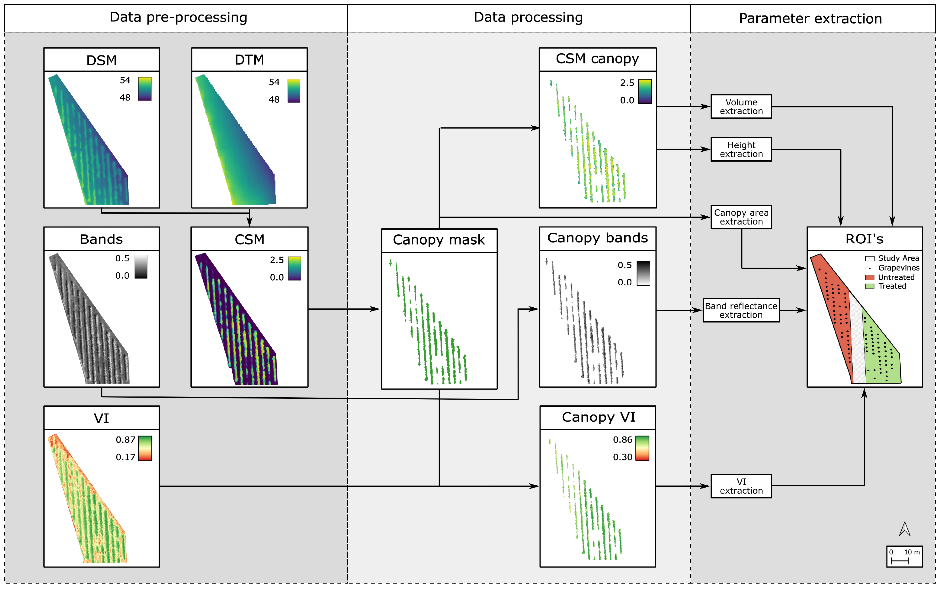
2.2.2. Data Processing

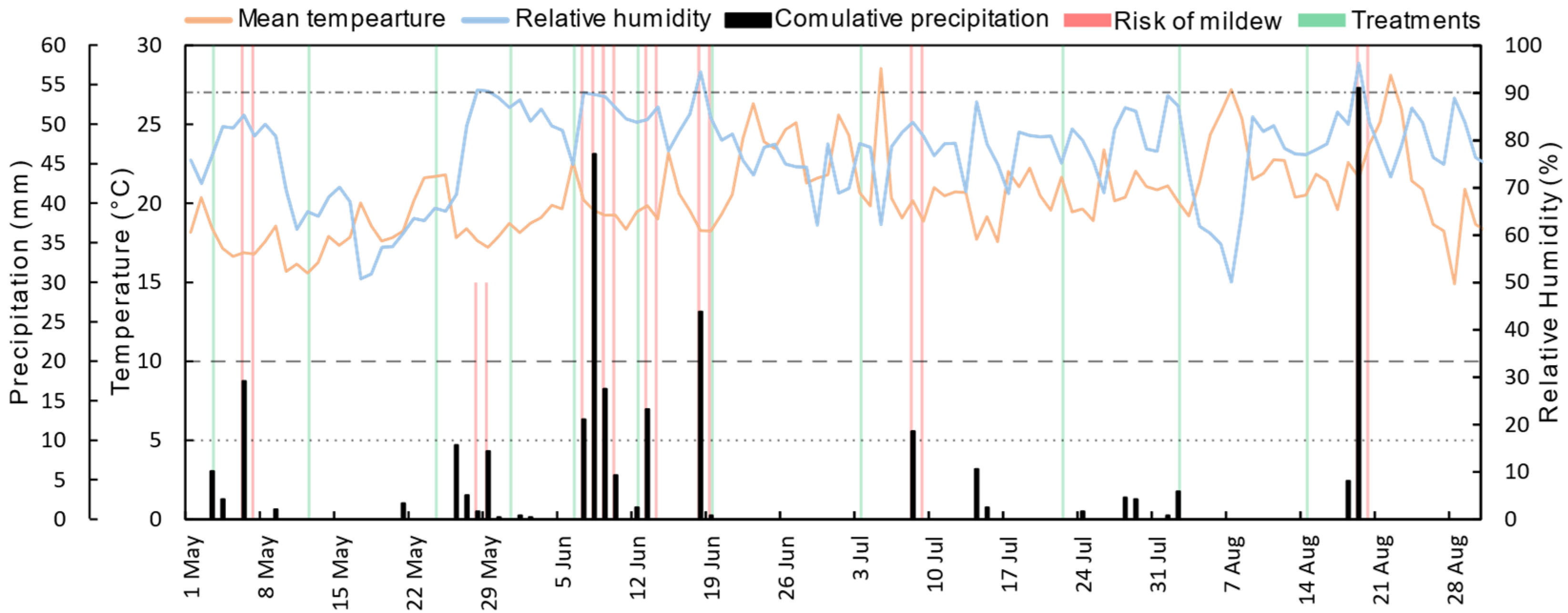
UAV imagery was processed using Pix4Dmapper Pro (version 4.5.6, Pix4D SA, Lausanne, Switzerland). This software employs Structure from Motion (SfM) algorithms to identify common points across the images. The initial processing step was performed for the calibration of internal and external camera parameters and for the computation of tie points, resulting in a sparse point cloud. GCPs were used to ensure data alignment over the different periods. An overall root mean square error (planimetric and altimetric) of 0.045 m for the RGB imagery and 0.056 m for the multispectral imagery was obtained. Then, high-density point clouds were created, and the points were subsequently classified. In the final step, orthorectified raster products are generated, and the points from the dense point cloud are subjected to smoothing and noise filtering operations. Subsequently, the following outputs are generated: RGB orthophoto mosaics; digital terrain models (DTMs); digital surface models (DSMs); radiometrically calibrated multispectral bands; and VIs. To assess the impact of downy mildew on grapevine physiology, a set of VIs was selected based on their sensitivity to stress indicators such as chlorophyll degradation, leaf structural changes, and overall canopy vigor. The ten VIs selected in this study (

Table 2. Computed vegetation indices from multispectral imagery. B: blue; G: green; R: red; RE: red edge; NIR: near infrared.

Vegetation Index	Equation	Reference
Blue Normalized Difference Vegetation Index	$\mathrm{B}\mathrm{N}\mathrm{D}\mathrm{V}\mathrm{I}={\displaystyle \frac{\mathrm{N}\mathrm{I}\mathrm{R}-\mathrm{B}}{\mathrm{N}\mathrm{I}\mathrm{R}-\mathrm{B}}}$	[56]
Normalized Green–Blue Difference Index	$\mathrm{G}\mathrm{B}\mathrm{D}\mathrm{I}={\displaystyle \frac{\mathrm{G}-\mathrm{B}}{\mathrm{G}-\mathrm{B}}}$	[57]
Green Normalized Difference Vegetation Index	$\mathrm{G}\mathrm{N}\mathrm{D}\mathrm{V}\mathrm{I}={\displaystyle \frac{\mathrm{N}\mathrm{I}\mathrm{R}-\mathrm{G}}{\mathrm{N}\mathrm{I}\mathrm{R}+\mathrm{G}}}$	[58]
Green–Red Vegetation Index	$\mathrm{G}\mathrm{R}\mathrm{V}\mathrm{I}={\displaystyle \frac{\mathrm{G}-\mathrm{R}}{\mathrm{G}+\mathrm{R}}}$	[59]
Normalized Difference Red-Edge	$\mathrm{N}\mathrm{D}\mathrm{R}\mathrm{E}={\displaystyle \frac{\mathrm{N}\mathrm{I}\mathrm{R}-\mathrm{R}\mathrm{E}}{\mathrm{N}\mathrm{I}\mathrm{R}+\mathrm{R}\mathrm{E}}}$	[60]
Normalized Difference Vegetation Index	$\mathrm{N}\mathrm{D}\mathrm{V}\mathrm{I}={\displaystyle \frac{\mathrm{N}\mathrm{I}\mathrm{R}-\mathrm{R}}{\mathrm{N}\mathrm{I}\mathrm{R}+\mathrm{R}}}$	[61]
Red-edge Green Index	$\mathrm{R}\mathrm{E}\mathrm{G}\mathrm{I}={\displaystyle \frac{\mathrm{R}\mathrm{E}-\mathrm{G}}{\mathrm{R}\mathrm{E}+\mathrm{G}}}$	[55]
Red-edge Red Index	$\mathrm{R}\mathrm{E}\mathrm{R}\mathrm{I}={\displaystyle \frac{\mathrm{R}\mathrm{E}-\mathrm{R}}{\mathrm{R}\mathrm{E}+\mathrm{R}}}$	[55]
Red-edge Blue Index	$\mathrm{R}\mathrm{E}\mathrm{B}\mathrm{I}={\displaystyle \frac{\mathrm{R}\mathrm{E}-\mathrm{B}}{\mathrm{R}\mathrm{E}+\mathrm{B}}}$	Adapted from REGI and RERI
Red–Blue Vegetation Index	$\mathrm{R}\mathrm{B}\mathrm{V}\mathrm{I}={\displaystyle \frac{\mathrm{R}-\mathrm{B}}{\mathrm{R}+\mathrm{B}}}$	[62]

) were chosen also based on previous UAV-based research focused on grapevine disease monitoring [24,55], identified as responsive to disease-induced vegetation stress (e.g., NDVI, GNDVI, GRVI, NDRE, REGI, and RERI). Additionally, VIs using the blue spectral band (BNDVI, GBVI, RBVI, and REBI) were also included, given that this spectral region is less frequently explored in vineyard studies due to sensor limitations, potentially offering new insights into spectral responses linked to disease stress. All selected VIs were based on two-band normalized differences, ensuring consistent value ranges and comparability.

Raster processing and geospatial analysis were conducted using QGIS (version 3.36.2). The crop surface model (CSM) was calculated to analyze grapevine canopy height and structure, enabling it to isolate the grapevine from soil and non-crop elements. This raster was obtained by computing the altitude difference between the DSM and the DTM.

By calculating the CSM, the heights of objects within the vineyard plot, including the grapevine canopy, vineyard row posts, and ground, were determined. This raster product was used to identify pixels with values corresponding to specific height values, enabling the generation of masks representing the grapevine canopy. The segmentation approach relied on simplified threshold-based masking applied to the CSM. While suitable for plot-scale studies, this method has limitations in terms of scalability for large-scale vineyard operations. To isolate the grapevine canopy, all pixels representing soil or vegetation between the rows were excluded. Only pixels with height values exceeding one meter are selected for the first flight campaign (18 May 2023), while for subsequent flight campaigns, a threshold of 1.10 m was considered to mitigate the effects from non-grapevine elements. The resulting raster masks have a value of one for grapevine vegetation, with non-grapevine pixels set as no data (NaN).

These masks were applied to filter all raster datasets, including VIs, individual spectral bands, and CSMs, by multiplying them with the masks. Additionally, data related to grapevine canopy geometric development, such as canopy area and project canopy volume, were extracted. It should be noted that the CSM-based approach used for grapevine projected volume estimation does not differentiate individual structural elements, such as leaves, branches, or canopy gaps, which may introduce some overestimation by incorporating both plant material and void space. Nonetheless, this methodology was chosen for its operational efficiency and demonstrated effectiveness in previous vineyard monitoring studies [21,63,64,65].

The final step of data extraction relies on using the 84 grapevines, 42 located in each block. A set of points was collected by using the GNSS receiver at the central part of each grapevine, and these points were used to create polygons measuring 2 × 2.5 m (Figure 2). Additionally, general polygons were created for the whole study area, as well as for the two zones. The mean value of each band, VI, and geometric parameter were then extracted for each polygon.

2.3. Climate Data

Monitoring meteorological and environmental conditions is an effective approach for detecting the occurrence of fungal diseases such as downy mildew through the use of specific sensors to identify conditions conducive to pathogen development [66]. Data on air humidity, air temperature, and precipitation can be collected using these sensors. In the case of grapevines, an empirical method can be used to predict the occurrence of infections in vineyards [5,67], with a known grapevine shoot length. The probability of downy mildew occurrence can be categorized as low, medium, or high based on interactions between air temperature; precipitation, relative humidity; and grapevine shoot length of at least 0.1 m. A low probability is predicted when air temperature is below 10 °C, relative humidity exceeds 90%, and shoot length is less than 0.1 m. A medium probability is assigned when air temperature is below 10 °C, combined with either precipitation exceeding 10 mm or relative humidity above 90%, and shoot length at least 0.1 m. A high probability is determined when air temperature is above 10 °C, shoot length is at least 0.1 m, and either precipitation reaches 10 mm or more or relative humidity is 90% or higher.

To analyze the incidence of downy mildew throughout the study period, meteorological data were obtained from a weather station (Vantage Pro2 Plus, Davis Instruments, Hayward, CA, USA) located 140 m from the study area.

2.4. Phytosanitary Treatments

Disease control treatments were applied with 15-day intervals; this decision was made by the producer and aligns with standard regional practices in the Vinho Verde region. However, some control treatments were occasionally applied before predicted precipitation, as this condition is an important factor for disease spread. The substances applied for fungal disease control were selected to minimize cross-resistance development, and each active substance was used within its allowable limits. The control treatments and active substances are presented in

Table 3. Dates and active substances used in the control treatment of the study area.

Application Date	Difference (Days)	Active Substance
10 April 2023	—	Fosetyl-Al
25 April 2023	15	Fosetyl-Al
3 May 2023	8	Metalaxyl
12 May 2023	9	Cymoxanil and folpet
24 May 2023	12	Folpet and iprovalicarb
31 May 2023	7	Cymoxanil and folpet
6 June 2023	6	Cymoxanil and folpet
12 June 2023	6	Metalaxyl-M and folpet
19 June 2023	7	Cymoxanil and folpet
3 July 2023	14	Copper oxychloride and iprovalicarb
22 July 2023	19	Cimoxanil and folpet
2 August 2023	11	Copper sulfate and calcium
14 August 2023	12	Copper sulfate and calcium

.

2.5. Statistical and Data Analysis

To analyze data normality, an exploratory analysis was conducted using IBM SPSS Statistics version 29.0.2.0 (IBM Corp., Armonk, NY, USA). Graphical visualizations, including histograms and Q-Q plots, were generated, and descriptive statistics such as skewness and kurtosis were calculated. The preliminary assessment indicated that the data did not follow a normal distribution. Consequently, a non-parametric Kolmogorov–Smirnov (K-S) test was performed. This test does not assume normality and evaluates whether the data conform to a specific distribution. The K-S test is applied as follows:

$$D=\underset{x}{\sup }\left|\left.F_n\left(x\right)-F\left(x\right)\right|\right.,$$

(1)

where D is the test statistic, sup denotes the supremum (the maximum absolute value of the differences between the empirical cumulative distribution F_n(x) and the theoretical cumulative distribution F(x)). This measures the largest deviation between the observed and expected distributions, assessing the goodness of fit between the sample data and the theoretical distribution.

In addition to normality testing, the relationship among variables for all grapevines in each flight campaign and across all flight campaigns for both treated and untreated grapevines was evaluated using the Pearson correlation coefficient (r) and its significance (p-value) to test the hypothesis of no correlation against the alternative hypothesis of a nonzero correlation.

Moreover, data dispersion around the mean per grapevine was also evaluated for both treated and untreated zones across all flight campaigns. Box plots were created for each zone and flight campaign to visualize data variability. For morphometric variables (canopy area, height, and projected volume), the mean values per treatment were analyzed and plotted to compare trends between treated and untreated grapevines. Similarly, for spectral bands (blue, green, red, red edge, and NIR), the mean values per treatment were calculated and plotted to assess reflectance differences. This analysis was extended to all VIs (Table 2), where mean values per treatment were compared across flight campaigns. Additionally, spatial variability was assessed by creating maps for the morphometric variables and NDVI, displaying the mean value for each grapevine. These maps provided a visual representation of the spatial distribution of vegetation health and structural parameters across the study area during each flight campaign.

3. Results

The results obtained from UAV-based multispectral data are presented for the multi-temporal analysis of the estimated parameters to monitor the impact of downy mildew on grapevines. The analyses focus on three main aspects: (i) the influence of the climatic conditions in the disease risk, (ii) structural changes in grapevine canopy development due to infection, and (iii) spectral and VI variations as indicators of disease progression.

3.1. Downy Mildew Forecasting from Climate Data and Treatments

A temporal analysis of the daily cumulative precipitation, average air temperature, and average relative humidity was conducted to assess the potential risk of downy mildew infection. Over a four-month period, during which the grapevine shoot length already exceeded 0.1 m, the risk of infection was evaluated, as presented in Figure 3. The evaluated period started in the beginning of May and lasted until the end of August, covering the flight campaigns (Table 1).

In the interval analyzed, precipitation periods occurred sporadically, with peaks observed on 6 May, between 7 and 9 June, between 13 and 18 June, and on 8 July and 19 August. Precipitation events clearly increase the fungal infection risk, as rainfall is a critical factor in the proliferation of downy mildew. The average daily temperature ranged between 15 °C (28 August) and 29 °C (5 July). Moderate to high temperatures, when combined with elevated humidity levels, can promote fungal development. Daily relative humidity showed variations, ranging between 50% (7 August) and 96% (19 August). High humidity is also crucial for the development of fungal infections; peaks around 90% (six days) coincided with a higher probability of downy mildew infection. This underscores the importance of humidity management in vineyards to prevent disease. While average daily temperature alone does not show a direct correlation with infection risk, moderate to high temperatures, when combined with high humidity, favor the development of downy mildew.

The frequency of the phytosanitary treatments (Table 3) was adjusted proactively in response to the climatic conditions favorable for downy mildew development, particularly before or after precipitation events that create humid microenvironments. This preventative strategy shows effectiveness, demonstrating a structured approach to disease management by aligning treatment timing with infection risk conditions.

3.2. Data Characterization

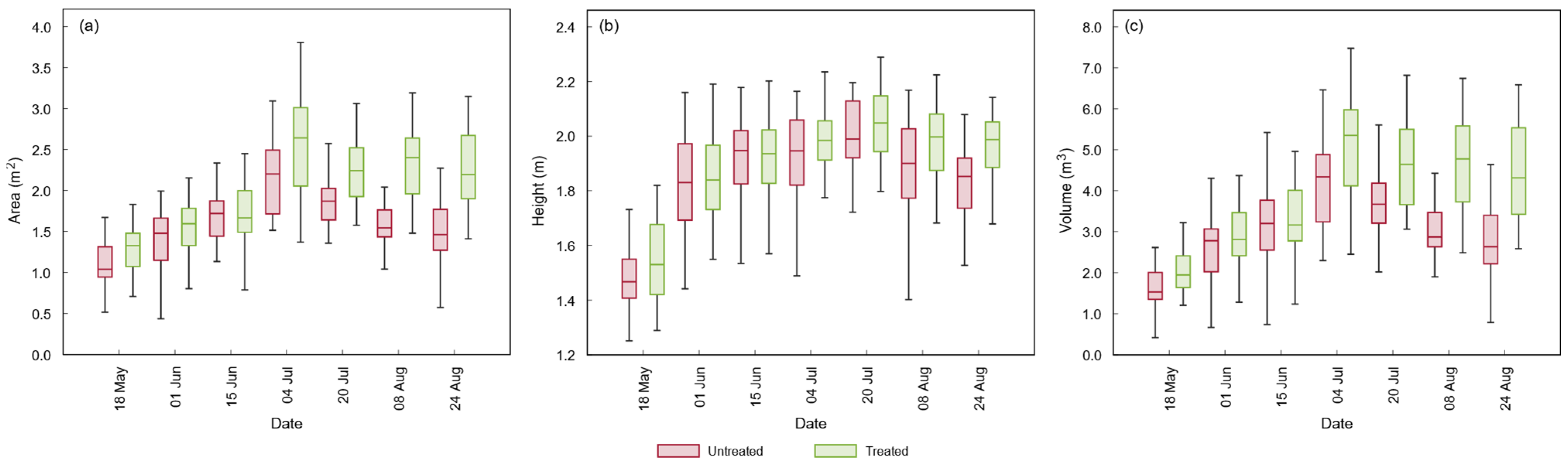
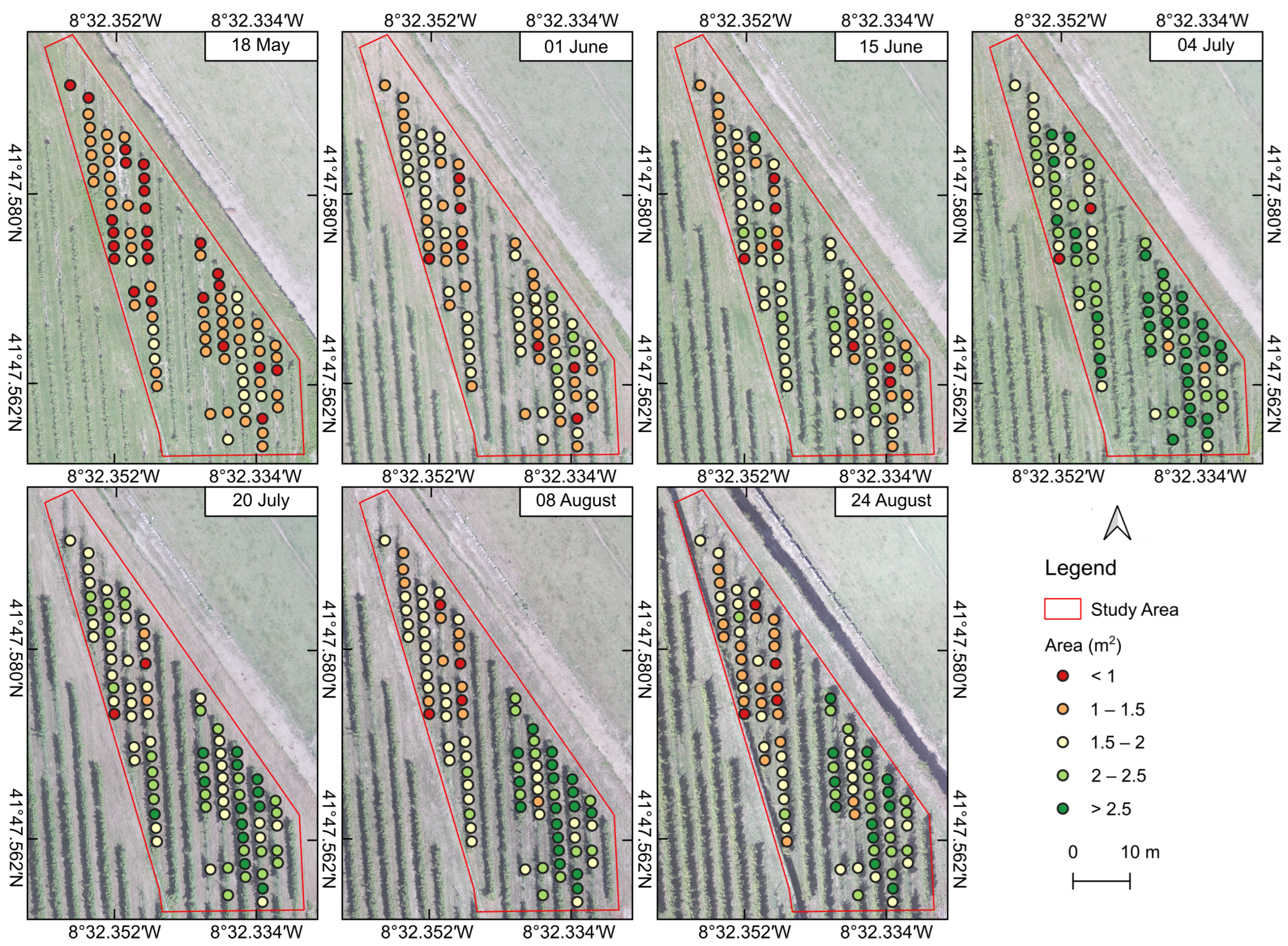
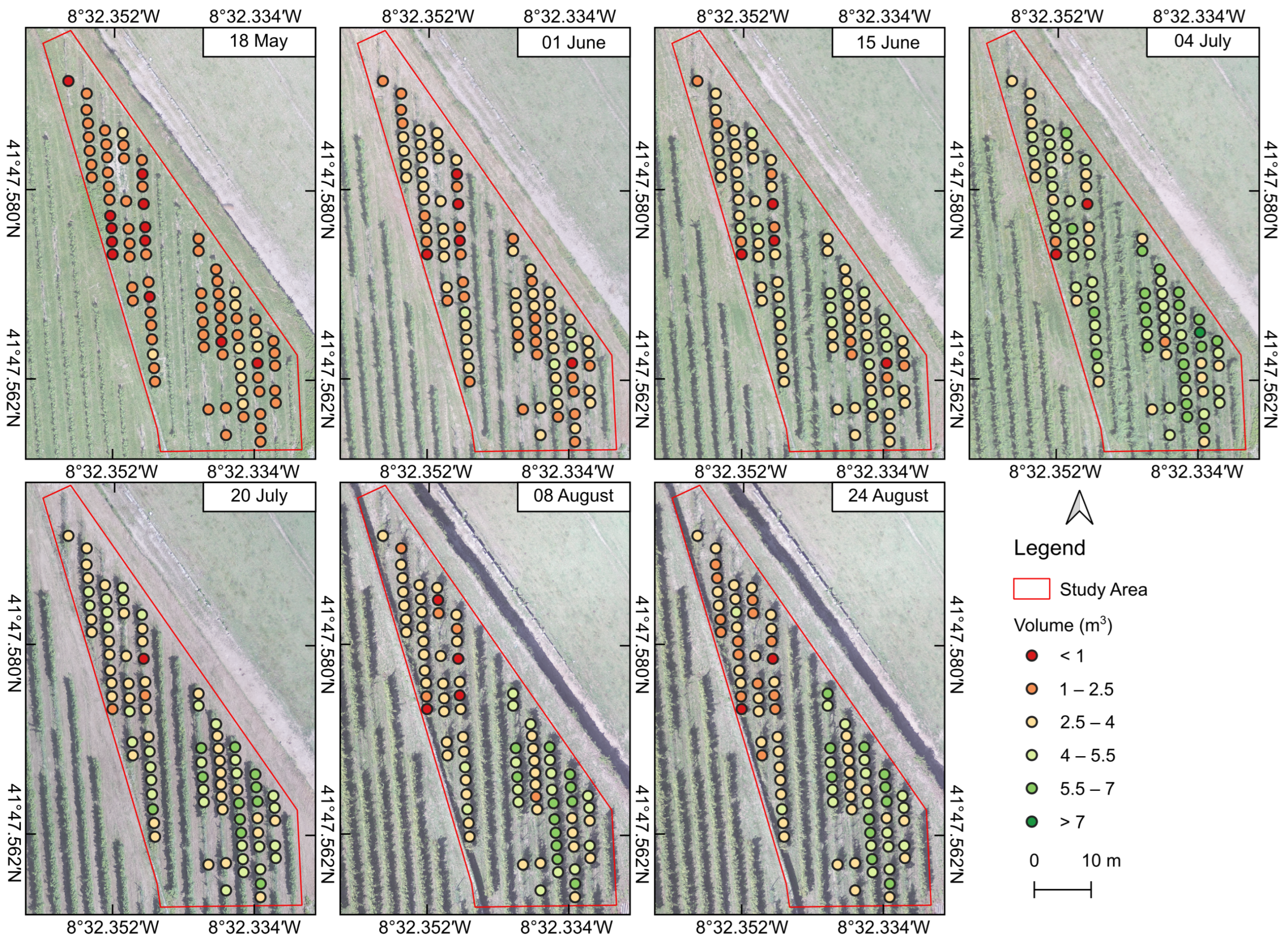
3.2.1. Morphometric Variables

The impact of downy mildew infection on the morphometric grapevine variables (canopy area, mean height, and projected volume) was analyzed across the treated (control) and untreated zones (Figure 4). Over time, there were noticeable differences between the two zones, with the untreated grapevines presenting a reduced canopy area (Figure 4a), lower plant height (Figure 4b), and smaller volume (Figure 4c), as demonstrated in the RGB point cloud data presented in Figure 5. The untreated grapevines showed a progressive reduction in canopy area (Figure 4a), with higher divergences from treated grapevines observed from July onwards. The projected canopy volume also declined in untreated plants (Figure 4c). Interestingly, the mean grapevine height (Figure 4b) did not show relevant differences until later stages. These results indicate that canopy area and volume are more reliable indicators of the downy mildew impact, particularly in the early to mid-stages of infection. Generally, grapevines in the treated zone show larger canopies, greater heights, and higher volumes than those in the untreated zone, indicating that the infection impacts grapevine growth and restricts its maximum development.

In the treated zone, the grapevine canopy area shows continuous growth, reaching its maximum on 4 July, when the median area exceeds 2.5 m². In the untreated zone, the grapevine canopy area is smaller, with the median only surpassing 2 m² on July 4, similarly to the control zone. The peak is observed on 4 July, but after this period, the median area declines through the time, while this value stabilizes for grapevines in the treated zone. A visual presentation of the individual canopy area of the evaluated grapevines is presented in Figure 6. In terms of mean grapevine height (Figure 4b), the control zone presents a consistent growth trend, stabilizing at around 2 m from 4 July onward, with the peak of the median value on 20 July. The plants maintain an average height above 1.8 m throughout the period. In contrast, grapevines in the untreated zone showed lower heights, starting slightly with plants barely reaching 2 m. After 20 July, the mean height of the untreated grapevines decreases in the subsequent flight campaigns, as presented in Figure 7. Among the morphometric variables, the grapevine projected volume shows the most evident differences between the two zones. In the treated zone, the grapevine volume increases over time, reaching peaks of over 6 m³ during July and August, indicating a continuous growth in both height and width (Figure 8). In the untreated zone, the canopy volume remains smaller, with the median values never exceeding 4.8 m³.

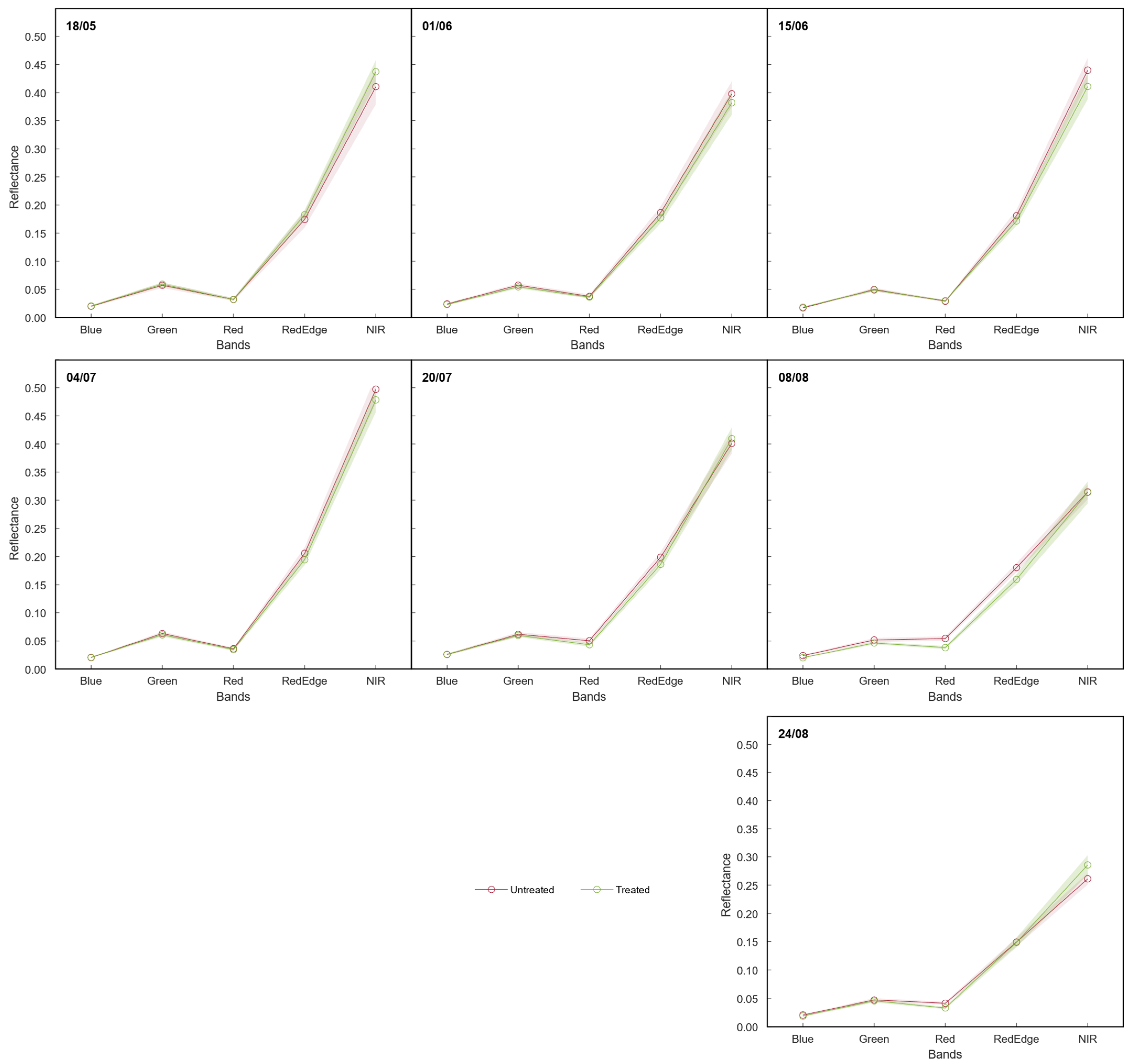
3.2.2. Spectral Reflectance

Reflectance values for the five spectral bands (blue, green, red, red edge, and NIR) were analyzed across the flight campaigns (Figure 9). In the first flight campaign (18 May), the mean spectral signatures of both zones were nearly identical, with minimal differences observed in the visible spectral bands (blue, green, red). However, control grapevines showed slightly higher reflectance values in the red-edge and NIR bands. On 1 June, similar results were observed, but the untreated grapevines showed higher mean reflectance values in the red edge and NIR bands compared to the control.

On 15 June and 4 July, the spectral response remained similar to 1 June, with the highest reflectance values observed on 4 July in the NIR band. By 20 July, a decrease in the reflectance values was observed in the red-edge and NIR bands, with the untreated grapevines showing higher reflectance values for red-edge and red bands. On 8 August, the difference between treated and untreated grapevines became more noticeable, particularly in the red and red-edge bands, with untreated grapevines showing higher reflectance in the visible bands. By 24 August, reflectance values decreased in all bands, with the NIR band showing the most decrease, with higher NIR values observed in treated grapevines, while lower reflectance was recorded in the red band.

Figure 9. Mean reflectance values of the spectral bands and its standard error for treated and untreated grapevines in each flight campaign.

Figure 9. Mean reflectance values of the spectral bands and its standard error for treated and untreated grapevines in each flight campaign.

Figure 10 presents the temporal variation in reflectance over time in the spectral bands for treated and untreated grapevines. These reflectance data show different patterns in spectral reflectance over time, which can reflect changes in leaf structure, pigment content, and infection progression. In the blue band (Figure 10a), reflectance increased from 18 May to 1 June, followed by a decline on 15 June, before peaking on 20 July (0.0259 in untreated and 0.0264 in treated grapevines). After this peak, which blue reflectance decreased in both zones, reaching 0.0203 in untreated and 0.0185 in treated grapevines on 24 August. As for the green band (Figure 10b), reflectance increased slightly in untreated grapevines from 18 May to 1 June but declined in treated grapevines. On 15 June, reflectance decreased in both zones; it increased again on 4 July and remained stable until 20 July. In the two subsequent periods, reflectance declined, reaching 0.0464 in untreated and 0.0452 in treated grapevines on 24 August. The red band (Figure 10c) showed more fluctuations compared to the blue and green bands. Reflectance increased between 18 May and 1 June, declined on 15 June, and increased again on 4 and 20 July. From 20 July to 8 August, red reflectance remained high in untreated grapevines (0.0554) but decreased in the treated grapevines (0.0379). By 24 August, reflectance declined in both groups to 0.0409 in untreated and 0.0329 in treated grapevines. The red-edge reflectance (Figure 10d) followed a similar trend to the green band. Between 18 May and 1 June, reflectance increased in untreated grapevines but slightly decreased in treated grapevines. A decline was observed in both zones on 15 June, followed by a peak on 4 July (0.2075 in untreated and 0.1963 in treated grapevines). In the subsequent flight campaigns, reflectance declined, reaching the lowest median values on 24 August (0.1497 in untreated, 0.1483 in treated). NIR reflectance (Figure 10e) decreased from 18 May to 1 June, followed by an increase until 4 July (0.4989 in untreated and 0.4807 in treated grapevines). From 20 July onward, a decline was observed in both zones, with untreated grapevines dropping to 0.2604 compared to 0.2870 for treated grapevines on 24 August.

Overall, untreated grapevines show higher reflectance than treated grapevines in the visible and red-edge bands in certain periods, with an example being 20 July, which may suggest an early structural change associated with infection. However, reflectance shows fluctuations, with initially higher values in untreated grapevines, followed by a decline after 20 July, which was more noticeable in the NIR and red-edge bands.

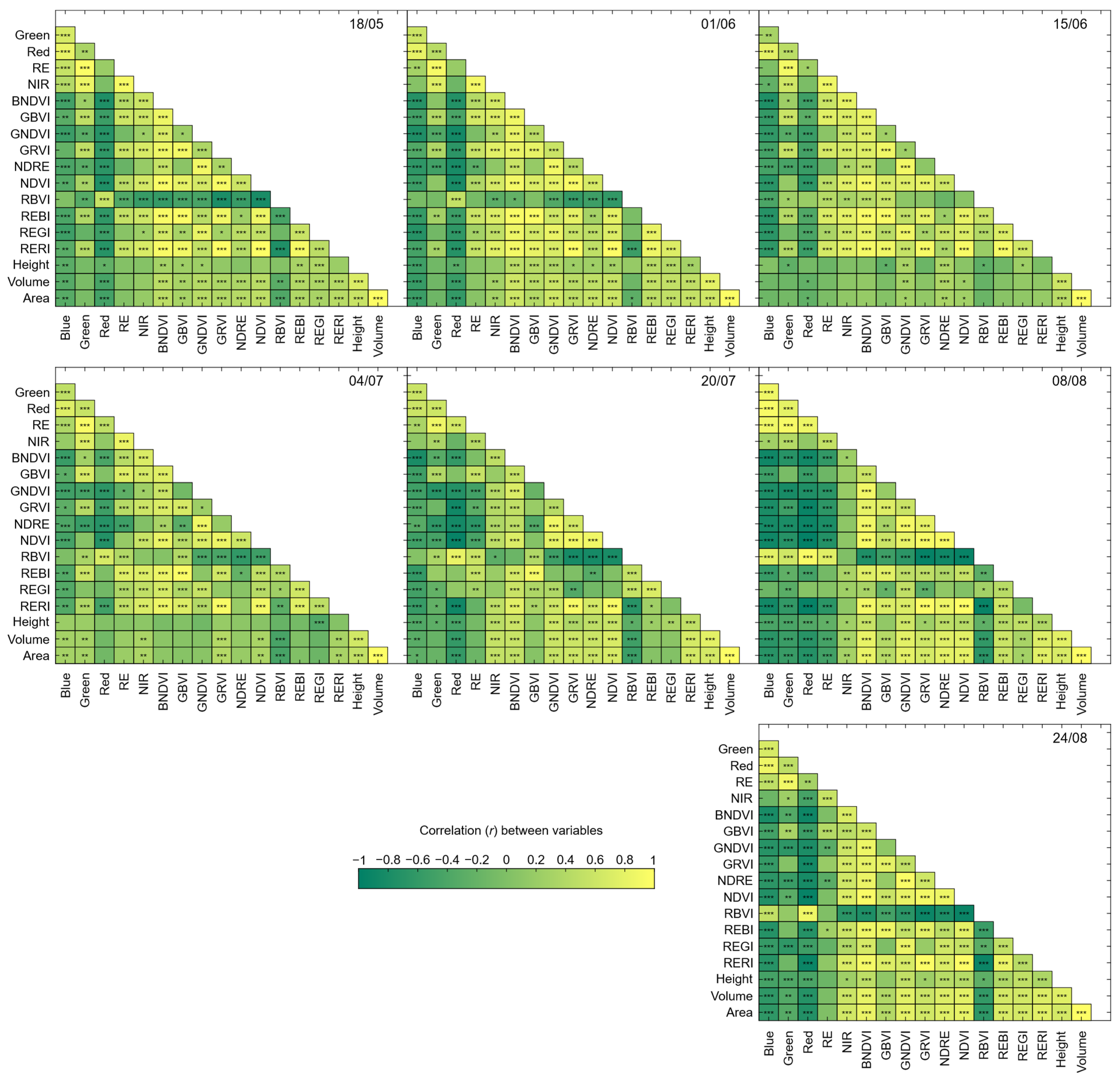
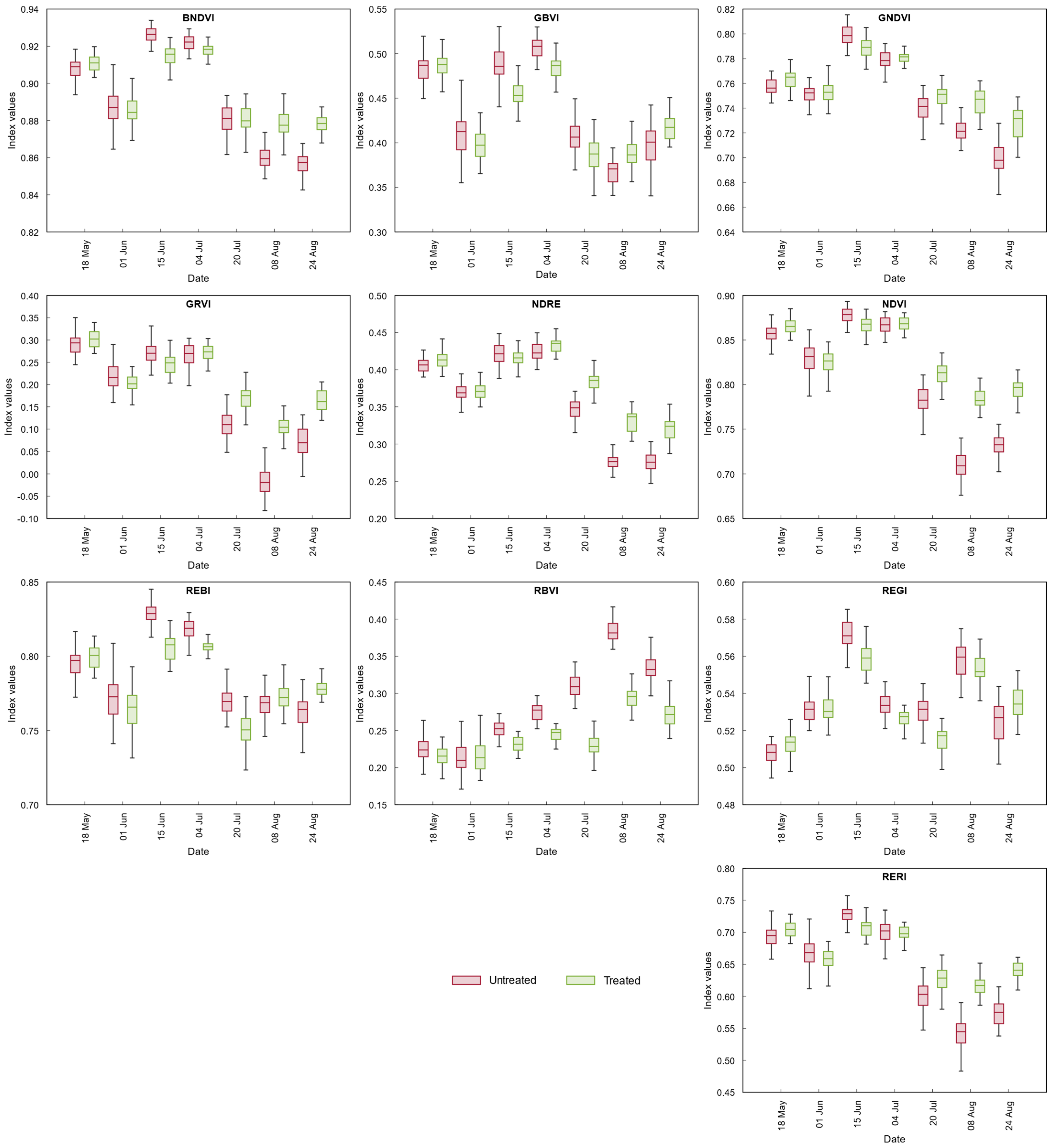
3.2.3. Vegetation Indices

Figure 11 presents the multi-temporal evolution of the evaluated VIs (Table 2) in treated and untreated grapevines. This analysis helps in the assessment of vegetation health status and the impact of downy mildew infection on grapevine canopy dynamics.

When analyzing VIs based on group-level trends, some indices demonstrate similar behavior throughout the study period. BNDVI, GBVI, and RERI showed higher median values in untreated grapevines from 1 June onward. However, in August, treated grapevines showed higher values in both flight campaigns. In contrast, GNDVI and NDRE followed a different pattern, with untreated grapevines showing higher values only on 15 June. After this period, treated grapevines either matched or slightly exceeded untreated values. GRVI and NDVI showed a similar trend, where untreated grapevines had higher values in June but declined by August, while treated grapevines maintained more stable values throughout the season. RERI followed a pattern similar to GRVI and NDVI, with untreated grapevines also showing higher values on 4 July. RBVI stood as the only VI where untreated grapevines showed higher values that treated ones, except on 1 June. REGI showed a mixed pattern, with untreated grapevines having higher median values in five campaigns (from 1 June to 8 August) before declining on 24 August.

The highest and lowest median values for each VI may be indicative of different trends in the spectral responses of untreated and treated grapevines. BNDVI reached its maximum median value in untreated grapevines on 15 June (0.93), while treated grapevines reached their median peak value earlier on 18 May (0.91). The lowest values for both groups occurred in August (0.86 and 0.88, respectively). GBVI showed its highest median value for untreated grapevines on 4 July (0.51), whereas for treated grapevines, it was on 18 May (0.49). The lowest median values were observed on 8 August (0.37 for untreated and 0.39 for treated grapevines).

Both GNDVI and NDRE followed similar trends, with maximum values occurring on 15 June for both untreated (0.80 and 0.42) and treated (0.79 and 0.44) grapevines, with their lowest values on 24 August (0.70 and 0.28 for untreated; 0.73 and 0.32 for treated). GRVI showed a contrast, reaching 0.29 in untreated grapevines on 18 May but declining to −0.02 on 8 August, whereas treated grapevines had a maximum median value at 0.30 on 18 May and declined to 0.10 on 8 August.

The maximum median value for RBVI was observed on 8 August (0.38 in untreated and 0.30 in treated grapevines) and reached its lowest values on 1 June (0.21 in untreated) and 18 May (0.22 in treated grapevines). REBI showed its highest median value on 15 June (0.83 in untreated and 0.81 in treated grapevines) and the lowest values on 24 August (0.76 in untreated and 0.75 in treated grapevines). REGI has peak median values on 15 June for both groups (0.57 for untreated and 0.56 for treated grapevines), with the lowest values on 18 May (0.51 in untreated) and 20 July (0.51 in treated grapevines). Similarly, RERI shows the highest median values on 15 June (0.73 in untreated and 0.71 in treated grapevines) and lowest values on 8 August (0.54 in untreated and 0.62 in treated grapevines).

NDVI reached its maximum median value on 15 June for both groups (0.88 in untreated and 0.87 in treated grapevines), with the lowest values observed on 8 August (0.71 in treated grapevines) and 24 August (0.78 in treated grapevines). The temporal variability in the mean NDVI values for each grapevine (Figure 12) shows the vegetative patterns across the season. Generally, grapevines show similar NDVI values in the first campaigns (18 May and 1 June), followed by slightly higher values in two mid-season campaigns (15 June and 4 July). However, a decline was observed in the last three campaigns, with treated grapevines showing a gradual NDVI decrease, while it was more abrupt in untreated plants.

3.3. Statistical Analysis of UAV-Based Parameters

The correlation between each parameter extracted from the UAV-based data is presented in Figure A1. When considering all flight campaigns (Figure 13a), a strong correlation was observed among spectral bands, with high correlations between blue and red (r = 0.94), red and green (r = 0.83), and green and red edge (r = 0.99). NIR reflectance also showed strong correlations with reflectance from red edge (r = 0.95) and green bands (r = 0.94) but slightly lower with blue (r = 0.80). Among VIs, strong correlations were observed between BNDVI and GNDVI, GBVI, NDRE, NDVI, and RERI (r > 0.88); between GBVI and REBI and RERI (r > 0.84); between GNDVI and NDRE (r = 0.90); between GRVI and NDVI and RERI (r > 0.88); between NDRE and NDVI (r = 0.95); and between RERI and NDVI and NDRE (r > 0.86). In contrast, RBVI and REGI did not show high positive or negative correlations with any other VI. Regarding geometric variables, the grapevine projected volume and canopy area were highly correlated (r = 0.98), while height showed moderate correlations with projected volume (r = 0.78) and canopy area (r = 0.67). Correlations between bands and VIs were strong, particularly for NIR reflectance with BNDVI (r = 0.91), GNDVI (r = 0.89), and REBI (r = 0.86). In contrast, correlations between geometric variables and spectral bands or VIs were minimal, with r values ranging between -0.18 and 0.23.

When considering only untreated grapevines (Figure 13b), spectral bands maintained high correlations (e.g., red edge and green with r = 0.99), though slightly lower than when considering all grapevines (Figure 13a). VIs showed stronger correlations among themselves, with BNDVI also showing a strong correlation with RERI (r = 0.88), GBVI with NDVI (r = 0.89), and GNDVI with NDVI and REBI (r > 0.86). Geometric variables maintained a strong correlation between projected volume and canopy area (r = 0.98), but the grapevine mean height was more strongly associated with the projected volume (r = 0.82) and canopy area (r = 0.71). Correlations between spectral bands and VIs remained high, particularly between NIR reflectance and BNDVI (r = 0.93), GNDVI (r = 0.91), and NDRE (r = 0.81), as well as between red-edge reflectance and REBI (r = 0.81). There was a slight increase in correlations between geometric variables and spectral bands and VIs, but those remained weak (ranging between −0.16 and 0.31).

Figure 13. Pearson correlation matrices and significance levels of the studied variables (spectral bands, vegetation indices, and geometric parameters) for all flight campaigns, considering all grapevines (a), grapevines in the untreated zone (b), and grapevines from the treated zone (c). Significance levels are indicated as follows: *, p < 0.05; **, p < 0.01; and ***, p < 0.001.

Figure 13. Pearson correlation matrices and significance levels of the studied variables (spectral bands, vegetation indices, and geometric parameters) for all flight campaigns, considering all grapevines (a), grapevines in the untreated zone (b), and grapevines from the treated zone (c). Significance levels are indicated as follows: *, p < 0.05; **, p < 0.01; and ***, p < 0.001.

In treated grapevines (Figure 13c), correlations among spectral bands were the highest (e.g., red and blue: r = 0.98; green and red edge: r = 0.99; NIR with red edge and green: r = 0.97; blue with green and red edge: r = 0.94; and red and red edge: r = 0.91). VIs maintained strong correlations, similar to those in untreated grapevines (Figure 13b), but with lower correlation values. Geometric variables again showed strong correlations between the projected volume and canopy area (r = 0.98), while grapevine height had the lowest correlations with these two parameters (r = 0.76 and r = 0.65 for projected volume and canopy area, respectively). Correlations between spectral bands and VIs were at their highest (e.g., NIR with GNDVI and BNDVI: r = 0.90; NIR with NDRE: r = 0.84; and red edge with BNDVI and GNDVI: r = 0.83). In contrast, correlations with geometric variables were minimal, ranging between −0.37 and 0.20.

The non-parametric K-S test results presented in

Table 4. Significance of the mean grapevine values between the two zones for each parameter. Significance levels are indicated as follows: n.s., p ≥ 0.05; *, p < 0.05; **, p < 0.01; and ***, p < 0.001.

Period	18 May	1 June	15 June	4 July	20 July	8 August	24 August
Blue	*	n.s.	***	n.s.	n.s.	***	***
Green	n.s.	***	n.s.	**	n.s.	***	n.s.
Red	n.s.	n.s.	*	**	***	***	***
Red Edge	***	**	***	***	***	***	n.s.
NIR	***	**	***	***	n.s.	n.s.	***
BNDVI	*	n.s.	***	***	n.s.	***	***
GBVI	n.s.	**	***	***	***	***	***
GNDVI	***	n.s.	***	n.s.	**	***	***
GRVI	n.s.	*	***	n.s.	***	***	***
NDRE	*	n.s.	n.s.	**	***	***	***
NDVI	*	n.s.	***	n.s.	***	***	***
RBVI	n.s.	n.s.	***	***	***	***	***
REBI	n.s.	n.s.	***	***	***	n.s.	***
REGI	**	n.s.	***	***	***	*	**
RERI	*	n.s.	***	n.s.	***	***	***
Height	n.s.	n.s.	n.s.	n.s.	n.s.	n.s.	***
Volume	*	n.s.	n.s.	***	***	***	***
Area	**	n.s.	n.s.	**	***	***	***

demonstrate statistically significant differences between treated and untreated grapevines across data from each flight campaign and different parameters. This statistical analysis confirmed significant differences in several parameters over time. VIs, particularly NDRE, NDVI, and REGI, demonstrated early differentiation between treated and untreated grapevines, with statistical significance detected as early as mid-June (p < 0.05). This reveals that multispectral VIs incorporating red-edge and near-infrared bands are effective in detecting early physiological stress caused by downy mildew.

The significance levels of the spectral bands varied throughout the study period. On 18 May, significant differences were observed in the red edge and NIR (p < 0.001) and the blue band (p < 0.05). On 1 June, the significance decreased, with green (p < 0.001) and red edge and NIR (p < 0.01) remaining statistically different. On 15 June and 4 July, statistical significance increased, with the exception being green (15 June) and blue (4 July) bands. On 20 July, only red and red edge showed a strong significant difference (p < 0.001). On 8 August, all bands except NIR showed a high degree of statistical significance (p < 0.001). On 24 August, this significance was no longer observed in the green and red-edge bands.

Compared to spectral bands, VIs showed a more stable statistical significance. On 18 May, significant differences were observed in BNDVI, NDRE, NDVI, RERI (p < 0.05), REGI (p < 0.01), and GNDVI (p < 0.001). An exception to the overall trend occurred on 1 June, where only GBVI (p < 0.01) and GRVI (p < 0.05) showed significant differences. From 15 June onwards, most VIs demonstrated significant differences. The only exceptions were NDRE (15 June), GNDVI, GRVI, NDVI, and RERI (4 July), BNDVI (20 July), and REBI (8 August). In the last flight campaign, all VIs demonstrated a statistically significant difference.

Unlike spectral bands and VIs, morphometric variables showed a delayed response, with significant differences becoming more pronounced in later phenological stages. For the mean grapevine height, no significant differences were observed in the first six flight campaigns, but statistical significance was detected on 24 August (p < 0.05). The canopy area and projected volume did not show statistically significant differences during the first two flight campaigns (p > 0.05). However, from July onward, both the canopy area and volume show highly significant differences (p < 0.01).

4. Discussion

The results of this study demonstrate the negative impact of downy mildew infection on grapevine growth and development, as reflected in the UAV-extracted parameters. The comparison between treated (control) and untreated grapevines over the growing season shows that infection leads to a decline in most analyzed metrics, which indicate a reduced plant health and vigor. These findings align with previous UAV-based disease-monitoring studies, such as Fuente et al. [15], who demonstrated that NDVI is effective in detecting vegetation stress. However, this study extends these findings by showing that VIs can provide earlier indications of downy mildew infection. Similarly, Pádua et al. [21] identified canopy volume as a relevant metric for monitoring grapevine development. In this study these results were confirmed by showing that canopy projected volume differences became statistically significant later in the season, reinforcing its utility for assessing the long-term impact. This is important for fungal diseases such as downy mildew, where early intervention is critical for effective management. By analyzing data from multiple time periods, this study provides a dynamic perspective on disease impact, rather than a static assessment at a single growth stage. Another advancement of this study is its integration of spectral, structural, and climatic data. This multi-dimensional analysis provides a more robust framework for precision agriculture applications, offering perspectives for winegrowers to optimize monitoring strategies and disease control.

The relationship between climatic factors and downy mildew infection risk is noticeable, particularly from May to June, when high humidity and precipitation coincided with an increased disease risk (Figure 3) [68]. Air temperature also contributed to establishing conditions for fungal proliferation, highlighting the need to enact climate monitoring for the implementation of proactive management strategies. The timing of the phytosanitary treatments aligned with weather conditions (precipitation events), demonstrating the effectiveness of integrating climatic risk assessment into vineyard disease management practices [69]. This approach not only helps in the mitigation of economic losses but could also reduce the number of treatments applied [70]. While this study considered climatic conditions to justify the timing and frequency of data acquisition, future studies would benefit from implementing generalized linear models or other multivariate modeling approaches. Such models could capture complex relationships between meteorological variables and disease incidence dynamics, improving the comprehensiveness of vineyard disease-monitoring strategies [68,71].

The results obtained for the different UAV-based metrics (Section 3.2) demonstrate the importance of integrating multispectral reflectance, VIs, and structural parameters to improve disease monitoring in vineyards. The geometric characteristics of grapevines were affected by the fungal infection (Section 3.2.1). Untreated grapevines showed a reduction in canopy area and volume, suggesting that downy mildew infection restricts lateral and vertical expansion (Figure 4). The findings on the impacts of observed vegetation development dynamics on the grapevine area (Figure 6) and projected volume (Figure 8) are similar to those in other studies, which show a peak during the same phenological stages [64]. While pruning and canopy management operations introduce variability between periods, the abrupt decline in untreated grapevines (Figure 4) when compared to control grapevines suggests that infection accelerates canopy deterioration compared to treated plants (Figure 1d), which show a low vegetative decline due to fruit maturation [21,46]. However, this decline was less evident in grapevine height when comparing the two zones (Figure 7). The inability of infected grapevines to achieve similar canopy growth as treated grapevines may reduce overall biomass production, potentially compromising crop productivity [72]. Differences in mean grapevine height between the two zones during August further indicate that downy mildew infection limits vertical growth, with untreated plants showing growth restrictions more noticeable from 20 July onward (Figure 4 and Figure 7). This suggests that downy mildew compromises structural integrity, potentially due to restricted nutrient transport, reduced photosynthetic efficiency, or direct tissue damage [73]. The variability observed among untreated grapevines suggests that downy mildew infection induces a more heterogeneous growth environment, where microclimatic variations, genetic differences, or infection severity may contribute to this variability. These results highlight the importance of developing disease management strategies to improve plant resistance [70].

Spectral reflectance analysis (Section 3.2.2) revealed significant physiological and structural changes in untreated grapevines due to downy mildew infection. An increase in reflectance in the visible bands (blue, green, and red) suggests reduced light absorption, likely caused by chlorophyll degradation and structural alterations in infected leaves (Figure 9). These results align with laboratory-based spectroscopy studies [74,75]. The reflectance increase in June and July coincides with certain phenological stages (Table 1), indicating that the infection was more impactful during these periods. The increase in blue reflectance, which can be an indicator of disease progression [76], suggests potential cell damage or tissue composition changes. In contrast, the more stable reflectance in treated grapevines indicates that phytosanitary treatments mitigated some of these effects [13]. Similarly, an increase in green reflectance in untreated grapevines can be related to modifications in leaf structure, pigment density, or water content, which contribute to higher reflectance [55]. These changes may indicate plant stress responses, such as cell degradation or the accumulation of phenolic compounds [24]. The decline in green reflectance from July 4 onward (Figure 10b) in treated and untreated grapevines suggests that phenological development and seasonal shifts in photosynthetic activity also had a contribution, raising the complexity of interpreting spectral data when both biotic and abiotic factors interact.

The red-edge band, sensitive to chlorophyll content, showed differences between treated and untreated grapevines, supporting the hypothesis that downy mildew infection reduces photosynthesis and directly affects the chlorophyll content and pigmentation [77,78,79]. The observed peaks in early July and early August, followed by a decline, may be related to plant acclimation or metabolic shifts as the infection progresses. The subsequent reduction in red-edge reflectance in the last flight campaign (Figure 10d) could reflect the seasonal declines in grapevine metabolic activity [5]. This is in line with the results reported by Wang et al. [80], where red-edge reflectance allowed the observation of physiological changes in grapevines. The NIR reflectance, which can be used to assess the leaf cell structure and water content [81], initially it showed higher reflectance in untreated grapevines, suggesting that infection may cause changes mesophyll cell compactness or water loss [82]. The subsequent decline in NIR reflectance over time (Figure 10e) may indicated plant adaptation to infection-induced stress [83] or phenological changes affecting both treated and untreated zones [84]. The differences between treated and untreated grapevines across most flight campaigns show that NIR reflectance has the potential to be used as a diagnostic metric for infection detection [82].

The use of VIs provided a robust approach for the assessment of the infection progression and treatment efficiency (Figure 11) [28,85]. VIs associated with leaf pigments and physiological status, such as BNDVI [81,86] and GBVI [87], showed a decline from mid-June onwards, indicative of the infection-induced stress. The increase in data dispersion suggests that downy mildew contributed to a heterogeneous stress response, whereas treated grapevines maintained higher and more stable values, demonstrating the effectiveness of phytosanitary treatments. Chlorophyll-related VIs such as GNDVI and NDRE [79] showed declines in untreated grapevines starting in mid-June, indicating chlorophyll degradation and reduced vegetative vigor [88]. NDRE proved to be sensitive at an intermediate infection stage, capturing chlorophyll changes before structural degradation. Kanaley et al. [89], Zottele et al. [83], and Daglio et al. [90] also confirm the NDRE usefulness in detecting infection-related photosynthetic efficiency loss, likely caused by tissue damage or vascular blockage. Similar trends are observed for NDVI, which diverged between treated and untreated grapevines from June onwards (Figure 12). The decline in NDVI among untreated grapevines suggests a reduction in vegetation density and photosynthetic activity due to downy mildew. In turn, VIs associated with structural degradation and vegetative vigor loss (e.g., GRVI, RBVI, REBI, REGI, and RERI) showed differentiation between treated and untreated grapevines from July onwards, making them useful for late-stage infection assessment [55]. The decline observed in REBI and RBVI, corresponding to the normalized difference in the blue and red edge, and blue and red reflectance, respectively, may be associated with changes in cell structure and pigment composition, particularly carotenoids and anthocyanins, which are essential for plant photoprotection [24,55].

These results highlight the importance and synergies of the normalized differences between the different spectral bands for continuous monitoring integrating multiple VIs to capture different aspects of plant stress, as no single index is sufficient to fully characterize disease impact. However, some temporal changes observed among the flight campaigns (Figure 11) are related to field interventions performed between some flight campaigns (1 June and 15 June), such as green pruning, defoliation, removal of new shoots, and vegetation management in the vineyard rows and between the rows; these operations impact multiple parameters since they change either the canopy geometry or overall leaf density, as already demonstrated in previous studies using multi-temporal data [21,46,64]. However, although this study focused on the grapevine growth period from May to August, covering stages when downy mildew impacts become significant and UAV-based assessments are feasible, extending the temporal coverage to include earlier phenological stages, such as bud burst, and later stages until senescence could provide a more complete understanding of disease dynamics. Future research should therefore consider extending the UAV monitoring period to capture the entire grapevine growth cycle, improving the applicability and robustness of the methodology.

The analysis of the correlations between UAV-based spectral bands and VIs demonstrated strong interdependencies (Figure 13 and Figure A1). Higher correlations among spectral bands in treated grapevines (Figure 13c) indicate a uniform and cohesive spectral response under healthier conditions. In contrast, untreated grapevines showed stronger correlations among VIs that share a common spectral band, thereby reducing physiological variability (Figure 13b). Geometric parameters demonstrated a strong intrinsic relationship between canopy area and grapevine projected volume, as expected due to their interdependence in volume calculations. However, distinct correlation patterns were observed between geometric and other parameters, except in untreated grapevines (Figure 13b). In these cases, correlations increased, possibly as some VIs began to capture structural aspects in addition to physiological ones. The weaker correlations observed in treated grapevines (Figure 13c) support the hypothesis that, under healthy conditions, grapevine structure is not directly reflected in simple spectral responses. This underscores the importance of assessing geometric parameter variability for a comprehensive understanding of grapevine conditions.

The statistical significance of different variable types over time highlights their potential effectiveness for early and late-stage detection of downy mildew in grapevines (Table 4). Some VIs showed early significance in detecting infection, with differences emerging on 18 May (BNDVI, GNDVI, and NDVI). Among the extracted metrics, VIs showed the most consistent trends throughout the study period, making them useful for early detection. In turn, spectral bands become more significant from June onward, particularly red edge and NIR, which show highly significant differences from 15 June to 24 August, indicating that pigment content and leaf structure changes due to infection are detectable from UAV-based multispectral data.

Morphometric variables showed significance later in the study period, with strong differentiation emerging on 4 July for canopy area and projected volume. These variables are better suited for assessing the long-term disease impact rather than early detection. While useful for confirming severity infection, they are less suitable for early-stage detection. Although the CSM-based method used for grapevine segmentation and canopy volume estimation provided data on grapevine canopy development and disease-induced morphological impacts, it did not fully account for the complex three-dimensional structure of grapevines. More precise methodologies, such as point-cloud volume estimation algorithms, could better account for the void spaces [91]. Future research should explore UAV photogrammetric or LiDAR point-cloud data for improved grapevine segmentation and volume estimation, enabling a better structural characterization and a deeper understanding of disease impacts on grapevine morphology.

Reproducing a similar multi-temporal study on powdery mildew would likely result in more pronounced differences in the UAV-based metrics extracted using multispectral data [92,93,94], as this fungal disease mainly affects the adaxial part of the leaves and grape clusters [5], making the impacts more measurable. Consequently, UAV-based remote-sensing metrics might capture its impact, to monitor earlier infection stages. Future research should focus on expanding spectral coverage and incorporating machine learning techniques [93,95] to improve early disease detection and vineyard management strategies. For machine learning, data fusion from different sensors should also be considered such as multispectral TIR-based features [12,92], and the inclusion of short-wave infrared [96] or textural features from RGB imagery [35,92]. Another alternative is the analysis of smaller canopy parts instead of individual grapevines; thus, the canopy is divided into multiple sections that are analyzed for each plant, which would allow for characterizing the infection along the vineyard rows. This type of approach was already applied for olive trees [31] and can be applied in vineyards though the integration object-based image analysis [34]. Moreover, the categorization of the infection severity is also essential for model development [34,36].

Despite the results provided by multispectral reflectance data, the spectral analysis in this study offers only a limited perspective on infection-induced physiological changes due to the restricted spectral resolution of the five-band sensor. Integrating additional data from TIR or hyperspectral sensors could improve disease monitoring. TIR data may enable the detection of stress-induced temperature variations at the canopy level, which could indicate pathogen presence and physiological impacts. Hyperspectral sensors, with improved spectral resolution, could improve the sensitivity and specificity of disease detection and characterization, particularly during early infection stages. Although such sensors were not used in this study, previous research conducted on the same plot using a handheld TIR sensor [97] has demonstrated their potential for detecting downy mildew symptoms (Figure 1c). Future research should explore multi-sensor data fusion, integrating multispectral, hyperspectral, and TIR data to develop a more robust disease assessment approach. These sensors can be used on aerial platforms, such as UAVs or satellites. In particular, UAV-based hyperspectral sensors or spectroradiometers could improve the detection of specific electromagnetic spectrum regions associated with disease progression [74,75,94,95]. This approach could improve the early identification of fungal diseases and their progression, supporting the development of precision viticulture strategies. Additionally, the emergence of hyperspectral satellite missions such as PRISMA has opened up new avenues for precision agriculture by enabling the acquisition of spectral signatures over larger spatial extents. Recent studies using PRISMA data have demonstrated the potential for early disease detection and improved crop management [98].

5. Conclusions

This study has demonstrated the effectiveness of UAV-based multi-temporal data monitoring of downy mildew progression in grapevines in a vineyard from a high-humidity region. The integration of multi-temporal data provided a dynamic assessment of disease impact, overcoming limitations associated with single UAV data acquisitions. The results confirm that UAV-based techniques are important tools for early disease detection and vineyard health monitoring.

The multi-temporal grapevine monitoring employed in this study allowed for the continuous monitoring of infection patterns and changes in the extracted parameters. The computed VIs showed a high sensitivity, highlighting their complementary role in disease monitoring. While some VIs are useful for early-stage infection, spectral bands are useful for tracking disease progression. Geometric variables demonstrated significant differences later in the season, making them more suitable for assessing long-term infection impacts rather than early detection.

The applicability of this methodology to other winegrowing regions is influenced by factors such as climate, grape variety, and cultivation practices. For instance, regions like Vinho Verde with denser canopy structures may reduce sensor penetration, potentially affecting the accuracy of UAV-based disease monitoring. Similarly, vineyard training systems with greater structural complexity, such as pergola, may require adjustments in UAV data acquisition, including flight height and sensor angle. Cost-effectiveness of UAV-based disease monitoring depends on operational factors, but the benefits in reducing fungicide applications make UAV-based monitoring a promising tool for precision viticulture.

These results reinforce the potential of UAV-based disease monitoring for vineyard management. Future studies should explore real-time data processing and artificial intelligence integration to automate detection and optimize treatment strategies. Expanding this methodology to other diseases, such as powdery mildew, Esca complex, Botrytis cinereal, viral diseases, or Flavescence dorée, could improve vineyard health management. Additionally, the integration of complementary remote-sensing technologies, such as hyperspectral imaging and TIR sensors, with artificial intelligence techniques may provide a more robust assessment of plant stress and disease severity. Incorporating multiple sensors, particularly TIR and hyperspectral sensors, could improve detection capabilities and provide a deeper understanding of grapevine disease dynamics. The flexibility of this methodology makes it applicable for other purposes, such as mapping grapevine heterogeneity or creating datasets for machine learning regression or classification, as each plant is georeferenced and can be directly associated with ground-truth data. These advancements contribute to an efficient disease-monitoring process, improving sustainability in viticulture by reducing fungicide applications and minimizing economic losses. Future research should focus on developing fully automated deep-learning grapevine canopy segmentation methods to improve scalability and facilitate its practical implementation in vineyard management.

References

1. Sishodia, R.P.; Ray, R.L.; Singh, S.K. Applications of Remote Sensing in Precision Agriculture: A Review. Remote Sens. 2020, 12, 3136. [Google Scholar] [CrossRef]
2. Ferro, M.V.; Catania, P. Technologies and Innovative Methods for Precision Viticulture: A Comprehensive Review. Horticulturae 2023, 9, 399. [Google Scholar] [CrossRef]
3. Tardaguila, J.; Stoll, M.; Gutiérrez, S.; Proffitt, T.; Diago, M.P. Smart Applications and Digital Technologies in Viticulture: A Review. Smart Agric. Technol. 2021, 1, 100005. [Google Scholar] [CrossRef]
4. Santesteban, L.G. Precision Viticulture and Advanced Analytics. A Short Review. Food Chem. 2019, 279, 58–62. [Google Scholar] [CrossRef]
5. Portela, F.; Sousa, J.J.; Araújo-Paredes, C.; Peres, E.; Morais, R.; Pádua, L. A Systematic Review on the Advancements in Remote Sensing and Proximity Tools for Grapevine Disease Detection. Sensors 2024, 24, 8172. [Google Scholar] [CrossRef]
6. Matese, A.; Filippo Di Gennaro, S. Technology in Precision Viticulture: A State of the Art Review. Int. J. Wine Res. 2015, 7, 69–81. [Google Scholar] [CrossRef]
7. Pádua, L.; Adão, T.; Hruška, J.; Sousa, J.J.; Peres, E.; Morais, R.; Sousa, A. Very High Resolution Aerial Data to Support Multi-Temporal Precision Agriculture Information Management. Procedia Comput. Sci. 2017, 121, 407–414. [Google Scholar] [CrossRef]
8. Brook, A.; De Micco, V.; Battipaglia, G.; Erbaggio, A.; Ludeno, G.; Catapano, I.; Bonfante, A. A Smart Multiple Spatial and Temporal Resolution System to Support Precision Agriculture from Satellite Images: Proof of Concept on Aglianico Vineyard. Remote Sens. Environ. 2020, 240, 111679. [Google Scholar] [CrossRef]
9. Cohen, B.; Edan, Y.; Levi, A.; Alchanatis, V. Early Detection of Grapevine (Vitis Vinifera) Downy Mildew (Peronospora) and Diurnal Variations Using Thermal Imaging. Sensors 2022, 22, 3585. [Google Scholar] [CrossRef]
10. Zia-Khan, S.; Kleb, M.; Merkt, N.; Schock, S.; Müller, J. Application of Infrared Imaging for Early Detection of Downy Mildew (Plasmopara Viticola) in Grapevine. Agriculture 2022, 12, 617. [Google Scholar] [CrossRef]
11. Araújo-Paredes, C.; Portela, F.; Mendes, S.; Valín, M.I. Using Aerial Thermal Imagery to Evaluate Water Status in Vitis Vinifera Cv. Loureiro. Sensors 2022, 22, 8056. [Google Scholar] [CrossRef] [PubMed]
12. Calderón, R.; Montes-Borrego, M.; Landa, B.B.; Navas-Cortés, J.A.; Zarco-Tejada, P.J. Detection of Downy Mildew of Opium Poppy Using High-Resolution Multi-Spectral and Thermal Imagery Acquired with an Unmanned Aerial Vehicle. Precis. Agric. 2014, 15, 639–661. [Google Scholar] [CrossRef]
13. Barjaktarovic, M.; Santoni, M.; Faralli, M.; Bertamini, M.; Bruzzone, L. A Multispectral Acquisition System for Potential Detection of Flavescence Dorée. In Proceedings of the 2022 30th Telecommunications Forum (TELFOR), Belgrade, Serbia, 15–16 November 2022; IEEE: New York, NY, USA, 2022; pp. 1–4. [Google Scholar]
14. Gennaro, S.D.; Battiston, E.; Marco, S.D.; Facini, O.; Matese, A.; Nocentini, M.; Palliotti, A.; Mugnai, L. Unmanned Aerial Vehicle (UAV)-Based Remote Sensing to Monitor Grapevine Leaf Stripe Disease within a Vineyard Affected by Esca Complex. Phytopathol. Mediterr. 2016, 55, 262–275. [Google Scholar] [CrossRef]
15. la Fuente, C.P.-D.; Valdés-Gómez, H.; Roudet, J.; Verdugo-Vásquez, N.; Mirabal, Y.; Laurie, V.F.; Goutouly, J.P.; Opazo, C.A.; Fermaud, M. Vigor Thresholded NDVI Is a Key Early Risk Indicator of Botrytis Bunch Rot in Vineyards. OENO One 2020, 54, 279–297. [Google Scholar] [CrossRef]
16. Sousa, J.J.; Toscano, P.; Matese, A.; Di Gennaro, S.F.; Berton, A.; Gatti, M.; Poni, S.; Pádua, L.; Hruška, J.; Morais, R.; et al. UAV-Based Hyperspectral Monitoring Using Push-Broom and Snapshot Sensors: A Multisite Assessment for Precision Viticulture Applications. Sensors 2022, 22, 6574. [Google Scholar] [CrossRef]
17. Gallo, R.; Ristorto, G.; Daglio, G.; Massa, M.; Berta, G.; Lazzari, M.; Mazzetto, F. New Solutions for the Automatic Early Detection of Diseases in Vineyards through Ground Sensing Approaches Integrating Lidar and Optical Sensors. Chem. Eng. Trans. 2017, 58, 673–678. [Google Scholar] [CrossRef]
18. Abdelghafour, F.; Keresztes, B.; Germain, C.; Da Costa, J.-P. In Field Detection of Downy Mildew Symptoms with Proximal Colour Imaging. Sensors 2020, 20, 4380. [Google Scholar] [CrossRef]
19. Tsouros, D.C.; Bibi, S.; Sarigiannidis, P.G. A Review on UAV-Based Applications for Precision Agriculture. Information 2019, 10, 349. [Google Scholar] [CrossRef]
20. Giovos, R.; Tassopoulos, D.; Kalivas, D.; Lougkos, N.; Priovolou, A. Remote Sensing Vegetation Indices in Viticulture: A Critical Review. Agriculture 2021, 11, 457. [Google Scholar] [CrossRef]
21. Pádua, L.; Marques, P.; Hruška, J.; Adão, T.; Peres, E.; Morais, R.; Sousa, J.J. Multi-Temporal Vineyard Monitoring through UAV-Based RGB Imagery. Remote Sens. 2018, 10, 1907. [Google Scholar] [CrossRef]
22. García-Fernández, M.; Sanz-Ablanedo, E.; Pereira-Obaya, D.; Rodríguez-Pérez, J.R. Vineyard Pruning Weight Prediction Using 3D Point Clouds Generated from UAV Imagery and Structure from Motion Photogrammetry. Agronomy 2021, 11, 2489. [Google Scholar] [CrossRef]
23. Ferro, M.V.; Catania, P.; Miccichè, D.; Pisciotta, A.; Vallone, M.; Orlando, S. Assessment of Vineyard Vigour and Yield Spatio-Temporal Variability Based on UAV High Resolution Multispectral Images. Biosyst. Eng. 2023, 231, 36–56. [Google Scholar] [CrossRef]
24. Albetis, J.; Duthoit, S.; Guttler, F.; Jacquin, A.; Goulard, M.; Poilvé, H.; Féret, J.-B.; Dedieu, G. Detection of Flavescence Dorée Grapevine Disease Using Unmanned Aerial Vehicle (UAV) Multispectral Imagery. Remote Sens. 2017, 9, 308. [Google Scholar] [CrossRef]
25. Mucalo, A.; Matić, D.; Morić-Španić, A.; Čagalj, M. Satellite Solutions for Precision Viticulture: Enhancing Sustainability and Efficiency in Vineyard Management. Agronomy 2024, 14, 1862. [Google Scholar] [CrossRef]
26. Aneece, I.; Thenkabail, P.S. New Generation Hyperspectral Sensors DESIS and PRISMA Provide Improved Agricultural Crop Classifications. Photogramm. Eng. Remote Sens. 2022, 88, 715–729. [Google Scholar] [CrossRef]
27. Guo, A.; Huang, W.; Dong, Y.; Ye, H.; Ma, H.; Liu, B.; Wu, W.; Ren, Y.; Ruan, C.; Geng, Y. Wheat Yellow Rust Detection Using UAV-Based Hyperspectral Technology. Remote Sens. 2021, 13, 123. [Google Scholar] [CrossRef]
28. Chatzidimopoulos, M.; Tsiouni, M.; Lagoudas, C.; Loridas, A.; Baliktsis, S.; Vozikis, C. Unmanned Aerial Systems for Early Detection of Downy Mildew in Tobacco Fields: Enhancing Financial Outcomes through Precision Monitoring. In Proceedings of the Tenth International Conference on Remote Sensing and Geoinformation of the Environment (RSCy2024), 13 September 2024; Volume 13212, pp. 398–401. [Google Scholar]
29. Garcia-Ruiz, F.; Sankaran, S.; Maja, J.M.; Lee, W.S.; Rasmussen, J.; Ehsani, R. Comparison of Two Aerial Imaging Platforms for Identification of Huanglongbing-Infected Citrus Trees. Comput. Electron. Agric. 2013, 91, 106–115. [Google Scholar] [CrossRef]
30. Ye, H.; Huang, W.; Huang, S.; Cui, B.; Dong, Y.; Guo, A.; Ren, Y.; Jin, Y. Recognition of Banana Fusarium Wilt Based on UAV Remote Sensing. Remote Sens. 2020, 12, 938. [Google Scholar] [CrossRef]
31. Castrignanò, A.; Belmonte, A.; Antelmi, I.; Quarto, R.; Quarto, F.; Shaddad, S.; Sion, V.; Muolo, M.R.; Ranieri, N.A.; Gadaleta, G.; et al. Semi-Automatic Method for Early Detection of Xylella Fastidiosa in Olive Trees Using UAV Multispectral Imagery and Geostatistical-Discriminant Analysis. Remote Sens. 2021, 13, 14. [Google Scholar] [CrossRef]
32. Chandel, A.K.; Khot, L.R.; Sallato, B.C. Towards Rapid Detection and Mapping of Powdery Mildew in Apple Orchards. In Proceedings of the 2020 IEEE International Workshop on Metrology for Agriculture and Forestry (MetroAgriFor), Trento, Italy, 4–6 November 2020; pp. 288–292. [Google Scholar]
33. Pádua, L.; Marques, P.; Martins, L.; Sousa, A.; Peres, E.; Sousa, J.J. Monitoring of Chestnut Trees Using Machine Learning Techniques Applied to UAV-Based Multispectral Data. Remote Sens. 2020, 12, 3032. [Google Scholar] [CrossRef]
34. Kuswidiyanto, L.W.; Wang, P.; Noh, H.-H.; Jung, H.-Y.; Jung, D.-H.; Han, X. Airborne Hyperspectral Imaging for Early Diagnosis of Kimchi Cabbage Downy Mildew Using 3D-ResNet and Leaf Segmentation. Comput. Electron. Agric. 2023, 214, 108312. [Google Scholar] [CrossRef]
35. Rodríguez-Gómez, J.P.; Di Cicco, M.; Nardi, S.; Nardi, D. Mapping Infected Crops Through UAV Inspection: The Sunflower Downy Mildew Parasite Case. In Proceedings of the Advances and Trends in Artificial Intelligence. From Theory to Practice, Graz, Austria, 9–11 July 2019; Wotawa, F., Friedrich, G., Pill, I., Koitz-Hristov, R., Ali, M., Eds.; Springer International Publishing: Cham, Switzerland, 2019; pp. 495–503. [Google Scholar]
36. Abdulridha, J.; Ampatzidis, Y.; Qureshi, J.; Roberts, P. Identification and Classification of Downy Mildew Severity Stages in Watermelon Utilizing Aerial and Ground Remote Sensing and Machine Learning. Front. Plant Sci. 2022, 13, 791018. [Google Scholar] [CrossRef] [PubMed]
37. Power, A.; Truong, V.K.; Chapman, J.; Cozzolino, D. From the Laboratory to The Vineyard—Evolution of The Measurement of Grape Composition Using NIR Spectroscopy towards High-Throughput Analysis. High-Throughput 2019, 8, 21. [Google Scholar] [CrossRef] [PubMed]
38. Kerkech, M.; Hafiane, A.; Canals, R.; Ros, F. Vine Disease Detection by Deep Learning Method Combined with 3D Depth Information. In Proceedings of the Image and Signal Processing, Marrakesh, Morocco, 4–6 June 2020; El Moataz, A., Mammass, D., Mansouri, A., Nouboud, F., Eds.; Springer International Publishing: Cham, Switzerland, 2020; pp. 82–90. [Google Scholar]
39. Molitor, D.; Baus, O.; Didry, Y.; Junk, J.; Hoffmann, L.; Beyer, M. BotRisk: Simulating the Annual Bunch Rot Risk on Grapevines (Vitis Vinifera L. Cv. Riesling) Based on Meteorological Data. Int. J. Biometeorol. 2020, 64, 1571–1582. [Google Scholar] [CrossRef]
40. Campos, J.; García-Ruíz, F.; Gil, E. Assessment of Vineyard Canopy Characteristics from Vigour Maps Obtained Using UAV and Satellite Imagery. Sensors 2021, 21, 2363. [Google Scholar] [CrossRef]
41. Franke, J.; Menz, G. Multi-Temporal Wheat Disease Detection by Multi-Spectral Remote Sensing. Precis. Agric. 2007, 8, 161–172. [Google Scholar] [CrossRef]
42. Marucci, A.; Colantoni, A.; Zambon, I.; Egidi, G. Precision Farming in Hilly Areas: The Use of Network RTK in GNSS Technology. Agriculture 2017, 7, 60. [Google Scholar] [CrossRef]
43. Kontogiannis, S.; Konstantinidou, M.; Tsioukas, V.; Pikridas, C. A Cloud-Based Deep Learning Framework for Downy Mildew Detection in Viticulture Using Real-Time Image Acquisition from Embedded Devices and Drones. Information 2024, 15, 178. [Google Scholar] [CrossRef]
44. Lowe, A.; Harrison, N.; French, A.P. Hyperspectral Image Analysis Techniques for the Detection and Classification of the Early Onset of Plant Disease and Stress. Plant Methods 2017, 13, 80. [Google Scholar] [CrossRef]
45. Roşcăneanu, R.; Streche, R.; Osiac, F.; Bălăceanu, C.; Suciu, G.; Drăgulinescu, A.M.; Marcu, I. Detection of Vineyard Diseases Using the Internet of Things Technology and Machine Learning Algorithms. Aerul si Apa. Compon. ale Mediu. 2022, 128–139. [Google Scholar] [CrossRef]
46. Pádua, L.; Marques, P.; Adão, T.; Guimarães, N.; Sousa, A.; Peres, E.; Sousa, J.J. Vineyard Variability Analysis through UAV-Based Vigour Maps to Assess Climate Change Impacts. Agronomy 2019, 9, 581. [Google Scholar] [CrossRef]
47. Zherdev, A.V.; Vinogradova, S.V.; Byzova, N.A.; Porotikova, E.V.; Kamionskaya, A.M.; Dzantiev, B.B. Methods for the Diagnosis of Grapevine Viral Infections: A Review. Agriculture 2018, 8, 195. [Google Scholar] [CrossRef]
48. Guo, Q.; Honesty, S.; Xu, M.L.; Zhang, Y.; Schoelz, J.; Qiu, W. Genetic Diversity and Tissue and Host Specificity of Grapevine Vein Clearing Virus. Phytopathology 2014, 104, 539–547. [Google Scholar] [CrossRef] [PubMed]
49. Kaur, L.; Sharma, S.G. Identification of Plant Diseases and Distinct Approaches for Their Management. Bull. Natl. Res. Cent. 2021, 45, 169. [Google Scholar] [CrossRef]
50. Singh, V.; Sharma, N.; Singh, S. A Review of Imaging Techniques for Plant Disease Detection. Artif. Intell. Agric. 2020, 4, 229–242. [Google Scholar] [CrossRef]
51. Sassu, A.; Gambella, F.; Ghiani, L.; Mercenaro, L.; Caria, M.; Pazzona, A.L. Advances in Unmanned Aerial System Remote Sensing for Precision Viticulture. Sensors 2021, 21, 956. [Google Scholar] [CrossRef]
52. Fraga, H.; Malheiro, A.C.; Moutinho-Pereira, J.; Santos, J.A. Climate Factors Driving Wine Production in the Portuguese Minho Region. Agric. For. Meteorol. 2014, 185, 26–36. [Google Scholar] [CrossRef]
53. Lorenz, D.H.; Eichhorn, K.W.; Bleiholder, H.; Klose, R.; Meier, U.; Weber, E. Growth Stages of the Grapevine: Phenological Growth Stages of the Grapevine (Vitis vinifera L. ssp. vinifera)—Codes and Descriptions According to the Extended BBCH Scale. Aust. J. Grape Wine Res. 1995, 1, 100–103. [Google Scholar] [CrossRef]
54. Gouveia, C.; Santos, R.B.; Paiva-Silva, C.; Buchholz, G.; Malhó, R.; Figueiredo, A. The Pathogenicity of Plasmopara Viticola: A Review of Evolutionary Dynamics, Infection Strategies and Effector Molecules. BMC Plant Biol. 2024, 24, 327. [Google Scholar] [CrossRef]
55. Albetis, J.; Jacquin, A.; Goulard, M.; Poilvé, H.; Rousseau, J.; Clenet, H.; Dedieu, G.; Duthoit, S. On the Potentiality of UAV Multispectral Imagery to Detect Flavescence Dorée and Grapevine Trunk Diseases. Remote Sens. 2018, 11, 23. [Google Scholar] [CrossRef]
56. Yang, C.; Everitt, J.H.; Bradford, J.M.; Murden, D. Airborne Hyperspectral Imagery and Yield Monitor Data for Mapping Cotton Yield Variability. Precis. Agric. 2004, 5, 445–461. [Google Scholar] [CrossRef]
57. KAWASHIMA, S.; NAKATANI, M. An Algorithm for Estimating Chlorophyll Content in Leaves Using a Video Camera. Ann. Bot. 1998, 81, 49–54. [Google Scholar] [CrossRef]
58. Gitelson, A.A.; Kaufman, Y.J.; Merzlyak, M.N. Use of a Green Channel in Remote Sensing of Global Vegetation from EOS-MODIS. Remote Sens. Environ. 1996, 58, 289–298. [Google Scholar] [CrossRef]
59. Sripada, R.P.; Heiniger, R.W.; White, J.G.; Meijer, A.D. Aerial Color Infrared Photography for Determining Early In-Season Nitrogen Requirements in Corn. Agron. J. 2006, 98, 968–977. [Google Scholar] [CrossRef]
60. Barnes, E.M.; Clarke, T.R.; Richards, S.E.; Colaizzi, P.D.; Haberland, J.; Kostrzewski, M.; Waller, P.; Choi, C.; Riley, E.; Thompson, T.; et al. Coincident Detection of Crop Water Stress, Nitrogen Status and Canopy Density Using Ground-Based Multispectral Data. In Proceedings of the 5th International Conference on Precision Agriculture, Bloomington, MN, USA, 16–19 July 2000; pp. 1–15. [Google Scholar]
61. Rouse, J.W.; Haas, R.H.; Deering, D.W.; Schell, J.A.; Harlan, J.C. Monitoring the Vernal Advancement and Retrogradation (Green Wave Effect) of Natural Vegetation; NASA: Washington, DC, USA, 1974.
62. Gitelson, A.A.; Kaufman, Y.J.; Stark, R.; Rundquist, D. Novel Algorithms for Remote Estimation of Vegetation Fraction. Remote Sens. Environ. 2002, 80, 76–87. [Google Scholar] [CrossRef]
63. Di Gennaro, S.F.; Matese, A. Evaluation of Novel Precision Viticulture Tool for Canopy Biomass Estimation and Missing Plant Detection Based on 2.5D and 3D Approaches Using RGB Images Acquired by UAV Platform. Plant Methods 2020, 16, 91. [Google Scholar] [CrossRef]
64. Stolarski, O.; Fraga, H.; Sousa, J.J.; Pádua, L. Synergistic Use of Sentinel-2 and UAV Multispectral Data to Improve and Optimize Viticulture Management. Drones 2022, 6, 366. [Google Scholar] [CrossRef]
65. Pádua, L.; Adão, T.; Sousa, A.; Peres, E.; Sousa, J.J. Individual Grapevine Analysis in a Multi-Temporal Context Using UAV-Based Multi-Sensor Imagery. Remote Sens. 2020, 12, 139. [Google Scholar] [CrossRef]
66. Hnatiuc, M.; Ghita, S.; Alpetri, D.; Ranca, A.; Artem, V.; Dina, I.; Cosma, M.; Abed Mohammed, M. Intelligent Grapevine Disease Detection Using IoT Sensor Network. Bioengineering 2023, 10, 1021. [Google Scholar] [CrossRef]
67. Mezei, I.; Lukić, M.; Berbakov, L.; Pavković, B.; Radovanović, B. Grapevine Downy Mildew Warning System Based on NB-IoT and Energy Harvesting Technology. Electronics 2022, 11, 356. [Google Scholar] [CrossRef]
68. Chen, M.; Brun, F.; Raynal, M.; Makowski, D. Forecasting Severe Grape Downy Mildew Attacks Using Machine Learning. PLoS ONE 2020, 15, e0230254. [Google Scholar] [CrossRef]
69. Kleb, M.; Merkt, N.; Zörb, C. New Aspects of In Situ Measurements for Downy Mildew Forecasting. Plants 2022, 11, 1807. [Google Scholar] [CrossRef] [PubMed]
70. Caffi, T.; Rossi, V.; Bugiani, R. Evaluation of a Warning System for Controlling Primary Infections of Grapevine Downy Mildew. Plant Dis. 2010, 94, 709–716. [Google Scholar] [CrossRef] [PubMed]
71. Madden, L.V.; Ellis, M.A.; Lalancette, N.; Hughes, G.; Wilson, L.L. Evaluation of a Disease Warning System for Downy Mildew of Grapes. Plant Dis. 2000, 84, 549–554. [Google Scholar] [CrossRef]
72. Fernandes de Oliveira, A.; Serra, S.; Ligios, V.; Satta, D.; Nieddu, G. Assessing the Effects of Vineyard Soil Management on Downy and Powdery Mildew Development. Horticulturae 2021, 7, 209. [Google Scholar] [CrossRef]
73. Fontaine, F.; Pinto, C.; Vallet, J.; Clément, C.; Gomes, A.C.; Spagnolo, A. The Effects of Grapevine Trunk Diseases (GTDs) on Vine Physiology. Eur. J. Plant. Pathol. 2016, 144, 707–721. [Google Scholar] [CrossRef]
74. Lacotte, V.; Peignier, S.; Raynal, M.; Demeaux, I.; Delmotte, F.; da Silva, P. Spatial–Spectral Analysis of Hyperspectral Images Reveals Early Detection of Downy Mildew on Grapevine Leaves. Int. J. Mol. Sci. 2022, 23, 10012. [Google Scholar] [CrossRef]
75. Hernández, I.; Gutiérrez, S.; Ceballos, S.; Iñíguez, R.; Barrio, I.; Tardaguila, J. Artificial Intelligence and Novel Sensing Technologies for Assessing Downy Mildew in Grapevine. Horticulturae 2021, 7, 103. [Google Scholar] [CrossRef]
76. Kerkech, M.; Hafiane, A.; Canals, R. Deep Leaning Approach with Colorimetric Spaces and Vegetation Indices for Vine Diseases Detection in UAV Images. Comput. Electron. Agric. 2018, 155, 237–243. [Google Scholar] [CrossRef]
77. Grishina, A.; Lysov, M.; Ageyeva, M.; Diakova, V.; Sherstneva, O.; Brilkina, A.; Vodeneev, V. Bacterial and Viral-Induced Changes in the Reflectance Spectra of Nicotiana Benthamiana Plants. Horticulturae 2024, 10, 1363. [Google Scholar] [CrossRef]
78. Bendel, N.; Kicherer, A.; Backhaus, A.; Klück, H.-C.; Seiffert, U.; Fischer, M.; Voegele, R.T.; Töpfer, R. Evaluating the Suitability of Hyper- and Multispectral Imaging to Detect Foliar Symptoms of the Grapevine Trunk Disease Esca in Vineyards. Plant Methods 2020, 16, 142. [Google Scholar] [CrossRef] [PubMed]
79. Simic Milas, A.; Romanko, M.; Reil, P.; Abeysinghe, T.; Marambe, A. The Importance of Leaf Area Index in Mapping Chlorophyll Content of Corn under Different Agricultural Treatments Using UAV Images. Int. J. Remote Sens. 2018, 39, 5415–5431. [Google Scholar] [CrossRef]
80. Wang, Y.M.; Ostendorf, B.; Pagay, V. Detecting Grapevine Virus Infections in Red and White Winegrape Canopies Using Proximal Hyperspectral Sensing. Sensors 2023, 23, 2851. [Google Scholar] [CrossRef] [PubMed]
81. Marques, P.; Pádua, L.; Sousa, J.J.; Fernandes-Silva, A. Assessing the Water Status and Leaf Pigment Content of Olive Trees: Evaluating the Potential and Feasibility of Unmanned Aerial Vehicle Multispectral and Thermal Data for Estimation Purposes. Remote Sens. 2023, 15, 4777. [Google Scholar] [CrossRef]
82. Vélez, S.; Barajas, E.; Rubio, J.A.; Pereira-Obaya, D.; Rodríguez-Pérez, J.R. Field-Deployed Spectroscopy from 350 to 2500 Nm: A Promising Technique for Early Identification of Powdery Mildew Disease (Erysiphe Necator) in Vineyards. Agronomy 2024, 14, 634. [Google Scholar] [CrossRef]
83. Zottele, F.; Crocetta, P.; Baiocchi, V. How Important Is UAVs RTK Accuracy for the Identification of Certain Vine Diseases? In Proceedings of the 2022 IEEE Workshop on Metrology for Agriculture and Forestry (MetroAgriFor), Perugia, Italy, 3 November 2022; IEEE: New York, NY, USA, 2022; pp. 239–243. [Google Scholar]
84. Calamita, F.; Imran, H.A.; Vescovo, L.; Mekhalfi, M.L.; La Porta, N. Early Identification of Root Rot Disease by Using Hyperspectral Reflectance: The Case of Pathosystem Grapevine/Armillaria. Remote Sens. 2021, 13, 2436. [Google Scholar] [CrossRef]
85. Liu, Y.; Su, J.; Zheng, Z.; Liu, D.; Song, Y.; Fang, Y.; Yang, P.; Su, B. GLDCNet: A Novel Convolutional Neural Network for Grapevine Leafroll Disease Recognition Using UAV-Based Imagery. Comput. Electron. Agric. 2024, 218, 108668. [Google Scholar] [CrossRef]
86. Marques, P.; Carvalho, R.; Fernandes-Silva, A. Preliminary Assessment of the Relationship between Pigments in Olive Leaves and Vegetation Indices. Proc. Latv. Acad. Sciences. Sect. B. Nat. Exact Appl. Sci. 2022, 76, 517–525. [Google Scholar] [CrossRef]
87. Solano-Alvarez, N.; Valencia-Hernández, J.A.; Vergara-Pineda, S.; Millán-Almaraz, J.R.; Torres-Pacheco, I.; Guevara-González, R.G. Comparative Analysis of the NDVI and NGBVI as Indicators of the Protective Effect of Beneficial Bacteria in Conditions of Biotic Stress. Plants 2022, 11, 932. [Google Scholar] [CrossRef]
88. Radócz, L.; Szabó, A.; Tamás, A.; Illés, Á.; Bojtor, C.; Ragán, P.; Vad, A.; Széles, A.; Harsányi, E.; Radócz, L. Investigation of the Detectability of Corn Smut Fungus (Ustilago Maydis DC. Corda) Infection Based on UAV Multispectral Technology. Agronomy 2023, 13, 1499. [Google Scholar] [CrossRef]
89. Kanaley, K.; Combs, D.B.; Paul, A.; Jiang, Y.; Bates, T.; Gold, K.M. Assessing the Capacity of High-Resolution Commercial Satellite Imagery for Grapevine Downy Mildew Detection and Surveillance in New York State. Phytopathology 2024, 114, 2536–2545. [Google Scholar] [CrossRef] [PubMed]
90. Daglio, G.; Cesaro, P.; Todeschini, V.; Lingua, G.; Lazzari, M.; Berta, G.; Massa, N. Potential Field Detection of Flavescence Dorée and Esca Diseases Using a Ground Sensing Optical System. Biosyst. Eng. 2022, 215, 203–214. [Google Scholar] [CrossRef]
91. Ferreira, L.; Sousa, J.J.; Lourenço, J.M.; Peres, E.; Morais, R.; Pádua, L. Comparative Analysis of TLS and UAV Sensors for Estimation of Grapevine Geometric Parameters. Sensors 2024, 24, 5183. [Google Scholar] [CrossRef] [PubMed]
92. Liu, Y.; Liu, G.; Sun, H.; An, L.; Zhao, R.; Liu, M.; Tang, W.; Li, M.; Yan, X.; Ma, Y.; et al. Exploring Multi-Features in UAV Based Optical and Thermal Infrared Images to Estimate Disease Severity of Wheat Powdery Mildew. Comput. Electron. Agric. 2024, 225, 109285. [Google Scholar] [CrossRef]
93. Zeng, T.; Fang, J.; Yin, C.; Li, Y.; Fu, W.; Zhang, H.; Wang, J.; Zhang, X. Recognition of Rubber Tree Powdery Mildew Based on UAV Remote Sensing with Different Spatial Resolutions. Drones 2023, 7, 533. [Google Scholar] [CrossRef]
94. Abdulridha, J.; Ampatzidis, Y.; Roberts, P.; Kakarla, S.C. Detecting Powdery Mildew Disease in Squash at Different Stages Using UAV-Based Hyperspectral Imaging and Artificial Intelligence. Biosyst. Eng. 2020, 197, 135–148. [Google Scholar] [CrossRef]
95. Zeng, T.; Wang, Y.; Yang, Y.; Liang, Q.; Fang, J.; Li, Y.; Zhang, H.; Fu, W.; Wang, J.; Zhang, X. Early Detection of Rubber Tree Powdery Mildew Using UAV-Based Hyperspectral Imagery and Deep Learning. Comput. Electron. Agric. 2024, 220, 108909. [Google Scholar] [CrossRef]
96. Acosta, M.; Pena, J.; Sherafat, A.; Gonzalez, C.; Sherman, T.; Bhandari, S.; Raheja, A. Investigating the Potential of UAV-Based Hyperspectral Sensor in Detecting Powdery Mildew in Grapes. In Proceedings of the Autonomous Air and Ground Sensing Systems for Agricultural Optimization and Phenotyping IX, National Harbor, MD, USA, 7 June 2024; SPIE: Bellingham, WA, USA; Volume 13053, pp. 26–34. [Google Scholar]
97. Portela, F.; Paredes, C.A.; Sousa, J.J.; Pádua, L. The Potential of Thermal Imaging to Assist Winemakers in the Detection of Downy Mildew in Vitis Vinifera Cv Loureiro. Procedia Comput. Sci. 2025, 256, 78–85. [Google Scholar] [CrossRef]
98. Dutta, A.; Tyagi, R.; Chattopadhyay, A.; Chatterjee, D.; Sarkar, A.; Lall, B.; Sharma, S. Early Detection of Wilt in Cajanus Cajan Using Satellite Hyperspectral Images: Development and Validation of Disease-Specific Spectral Index with Integrated Methodology. Comput. Electron. Agric. 2024, 219, 108784. [Google Scholar] [CrossRef]
Figure 2. Flowchart of the data-processing pipeline. DSM: digital surface model; DTM: digital terrain model; CSM: crop surface model: VI: vegetation index: ROIs: regions of interest.
Agronomy 15 00934 g002
Figure 3. Temporal analysis of weather factors: daily mean air temperature, daily mean relative humidity, daily cumulative precipitation, and identification of high-risk periods for downy mildew infection. The horizontal dashed lines represent the threshold values related with the downy mildew risk for cumulative precipitation (above 10 mm), air temperature (above 10 °C), and relative humidity (above 90%).
Agronomy 15 00934 g003
Figure 4. Morphometric variables: (a) canopy area, (b) mean height, and (c) projected volume of the grapevines in the control (treated zone) and in the untreated zone throughout the analyzed periods.
Agronomy 15 00934 g004
Figure 5. Graphical representation of the photogrammetric point cloud of grapevines subjected to treatments (a) and untreated grapevines (b).
Agronomy 15 00934 g005
Figure 6. Canopy area of each grapevine over the seven flight campaigns.
Agronomy 15 00934 g006
Figure 7. Mean height of each grapevine over the seven flight campaigns.
Agronomy 15 00934 g007
Figure 8. Projected canopy volume for each grapevine over the seven flight campaigns.
Agronomy 15 00934 g008
Figure 10. Box plots of spectral reflectance in blue (a), green (b), red (c), red edge (d), and near infrared (e) bands for treated and untreated grapevines across the analyzed period.
Agronomy 15 00934 g010
Figure 11. Box plot distribution of vegetation indices (BNDVI, GBVI, GNDVI, GRVI, NDRE, NDVI, RBVI, REBI, REGI, and RERI) for treated and untreated grapevines throughout the study period.
Agronomy 15 00934 g011
Figure 12. Mean normalized difference vegetation index (NDVI) of each grapevine over the analyzed period.
Agronomy 15 00934 g012