Appendix A
In order to determine the angle interval and the number of views for the greenhouse tomato plants point cloud model reconstruction, the standard Styrofoam balls (SSBs) were selected as measurement objects. Four white SSBs with diameters of 30, 40, 50, and 60 cm were selected. The above 2.2 3D reconstruction method was used to reconstruct the SSBs point cloud model. The 3D point cloud reconstruction accuracy data for the SSBs were analyzed using the following method. During the SSBs point cloud reconstruction experiment, the Kinect sensor was placed in three positions (
P1,
P2, and
P3). In addition, three combinations of AOVs, namely,
V3 (0°, 120°, and 240°),
V4 (0°, 90°, 180°, and 270°), and
V6 (0°, 60°, 120°, 180°, 240°, and 300°) were used. Statistical data included the relative average deviation and coefficient of variation between the reconstructed and measured values of the diameter (
DX) in the horizontal (X-axis) direction, the diameter (
DY) in the vertical (Y-axis) direction, the volume (
Vol), the coverage (
Cr) of the reconstructed point cloud, the distribution frequency of the set of distances (
HRS) between the reconstructed and reference point clouds of each SSB, the Hausdorff distance (
HD) between the reconstructed and reference point clouds, and the average (
Havg) and standard deviation (
Hstd) of the
HD set.
Here, Cr is the percentage of the surface area of the SSB covered by the reconstructed point cloud (%); Sstandardball is the surface area of the SSB (cm2); and SHD is the point cloud surface area for which the distance between the scanned and reconstructed point clouds is less than 5.00% of the diameter of the SSB (cm2).
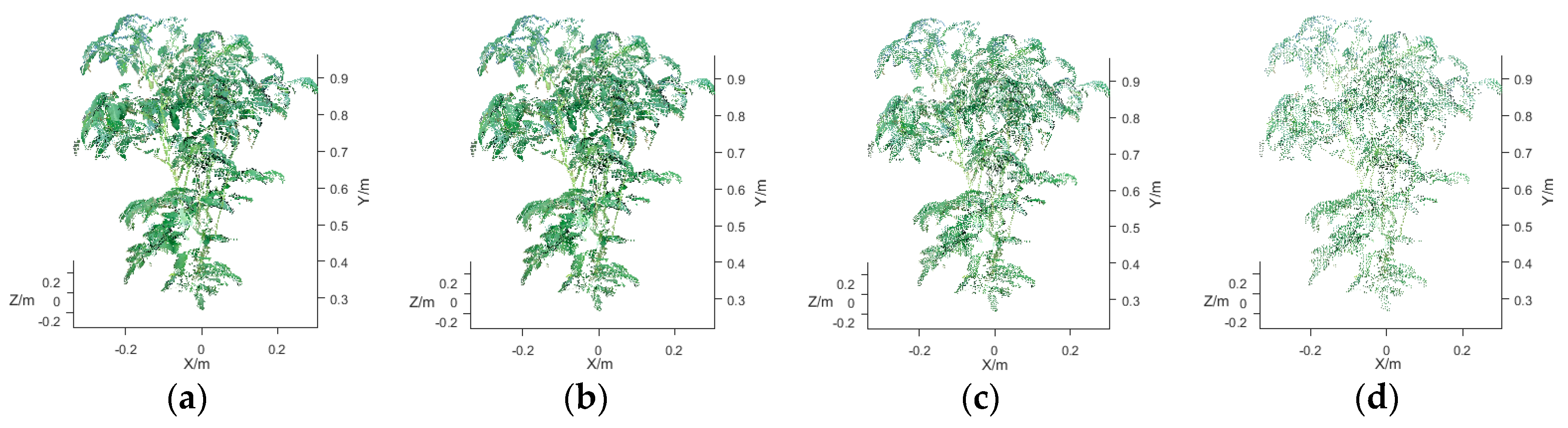
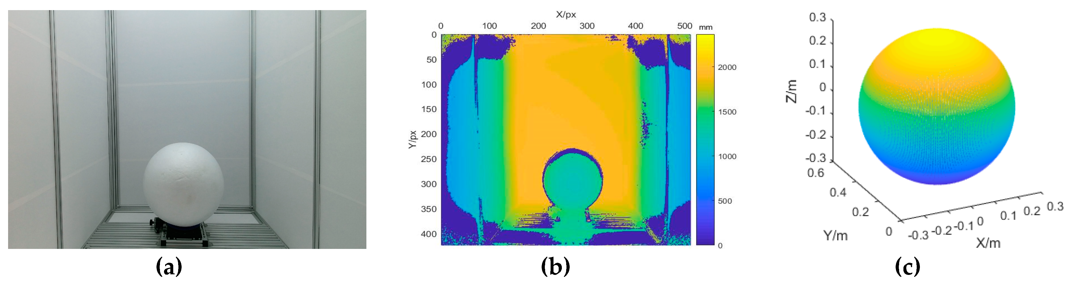
Figure A1a,b show an RGB color image and a depth image of an SSB, respectively. According to the 3D point cloud reconstruction process, 3D point clouds of the four SSBs with various diameters (30, 40, 50, and 60 cm) were reconstructed based on images captured by the Kinect sensor in three positions (
P1,
P2, and
P3) and at three combinations of AOVs (
V3,
V4, and
V6). In addition, a reference point cloud consisting of 90,000 points was constructed for each of the four SSBs.
Figure A1c shows the reference point cloud of the SSB with a diameter of 60 cm.
Figure A1.
Reconstruction of a 3D point cloud of the standard Styrofoam ball (SSB) with a diameter of 60 cm: (a) color image of the SSB; (b) depth image of the SSB; (c) reference point cloud of the SSB.
Figure A1.
Reconstruction of a 3D point cloud of the standard Styrofoam ball (SSB) with a diameter of 60 cm: (a) color image of the SSB; (b) depth image of the SSB; (c) reference point cloud of the SSB.
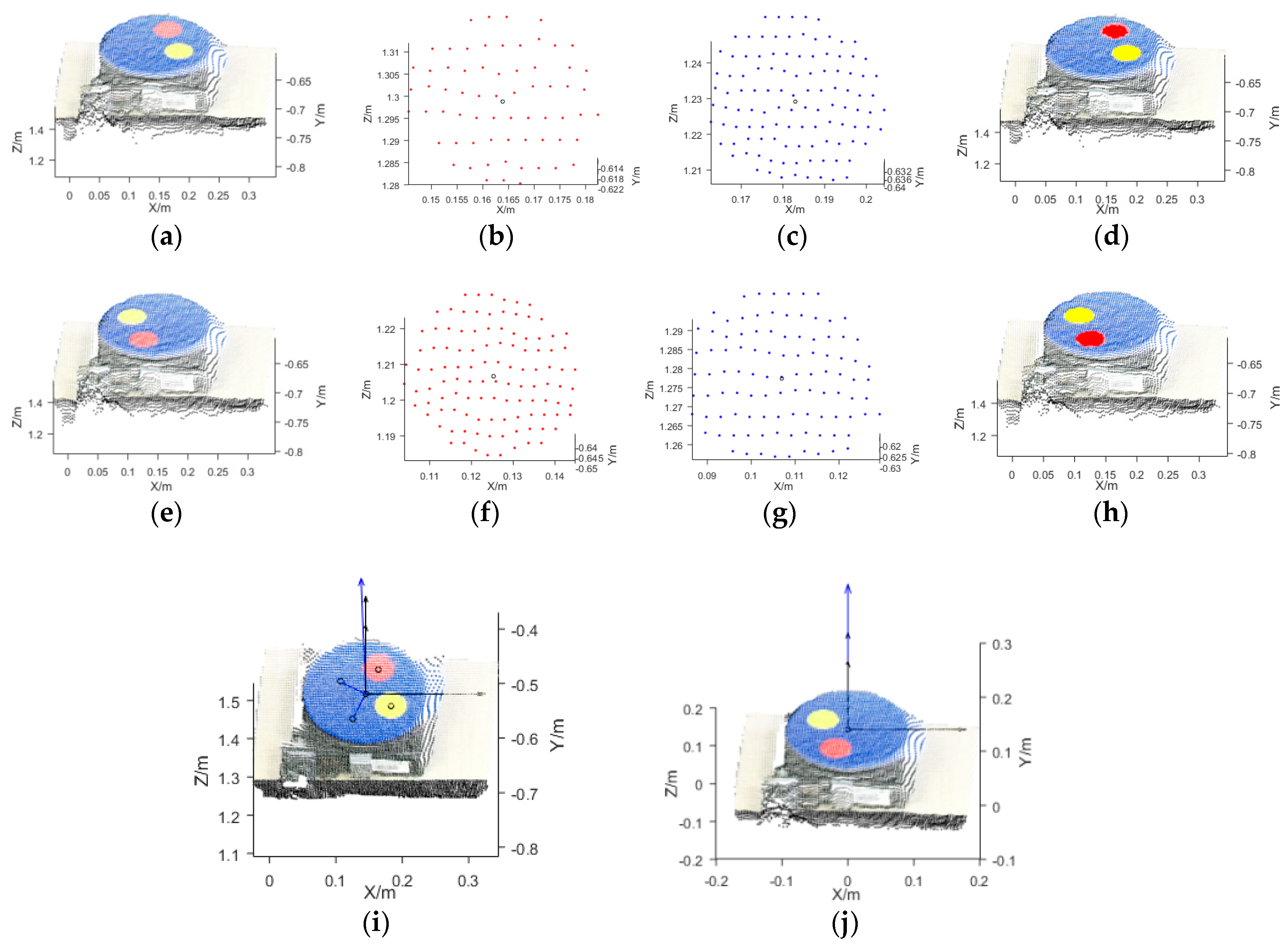
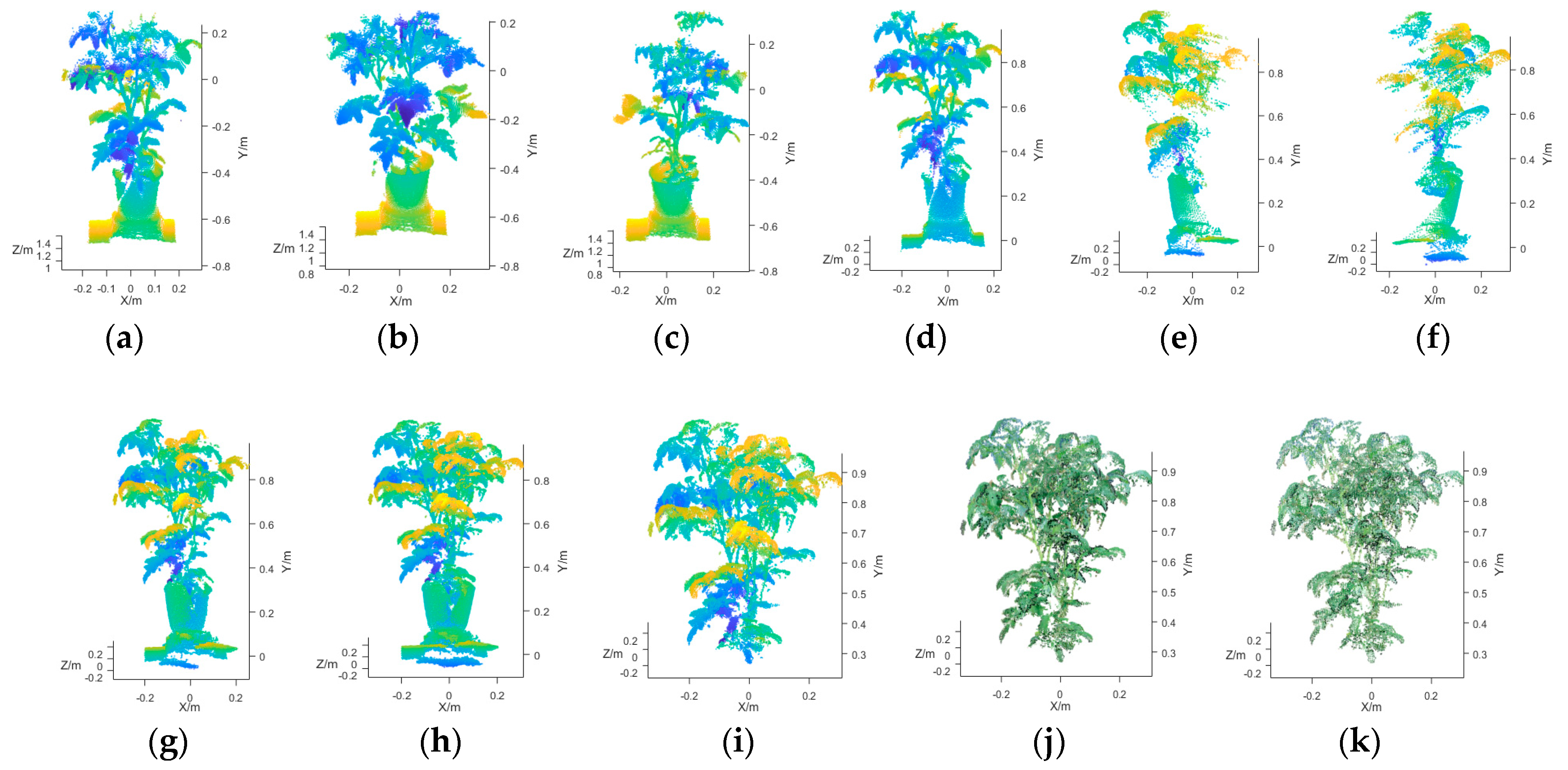
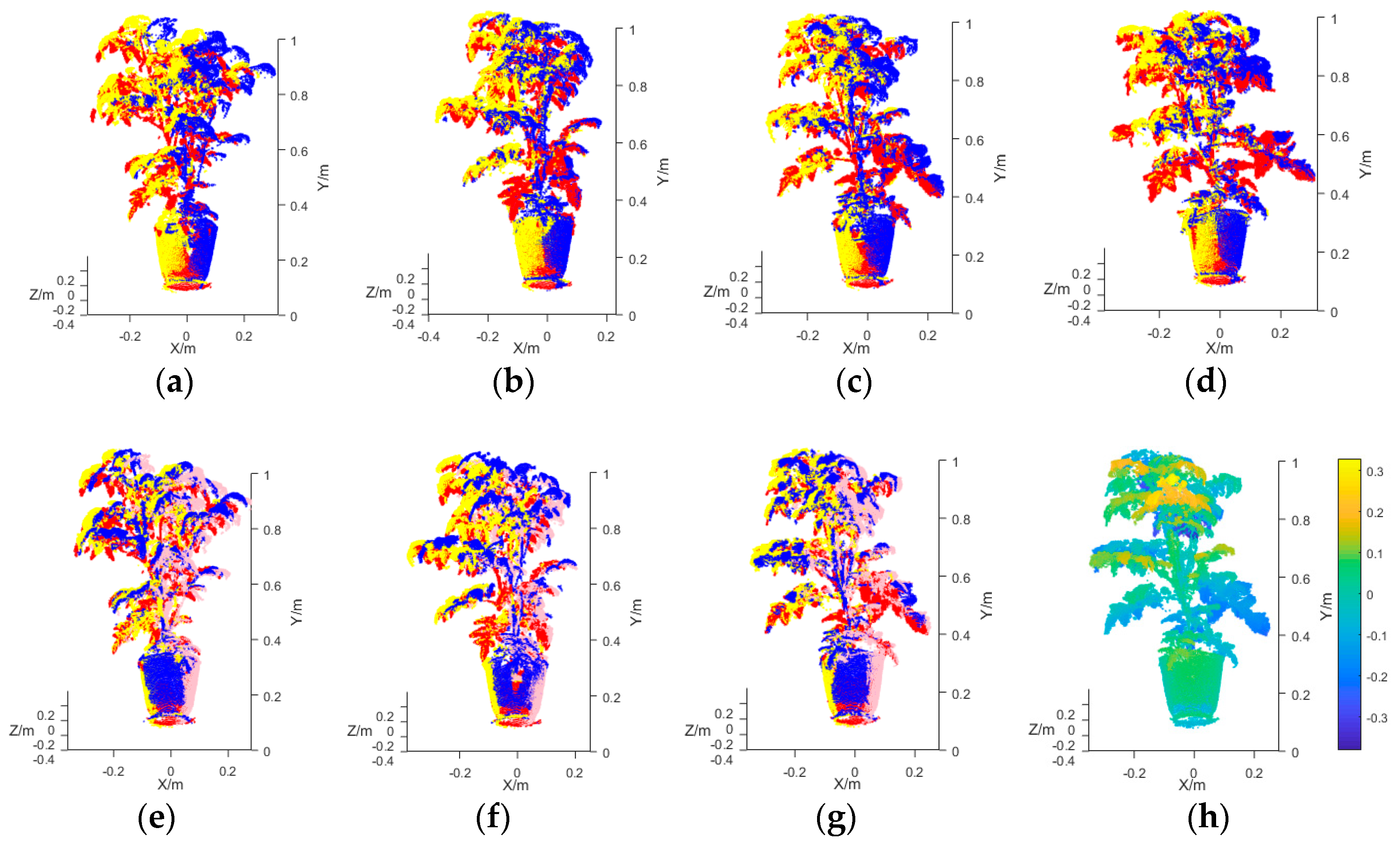
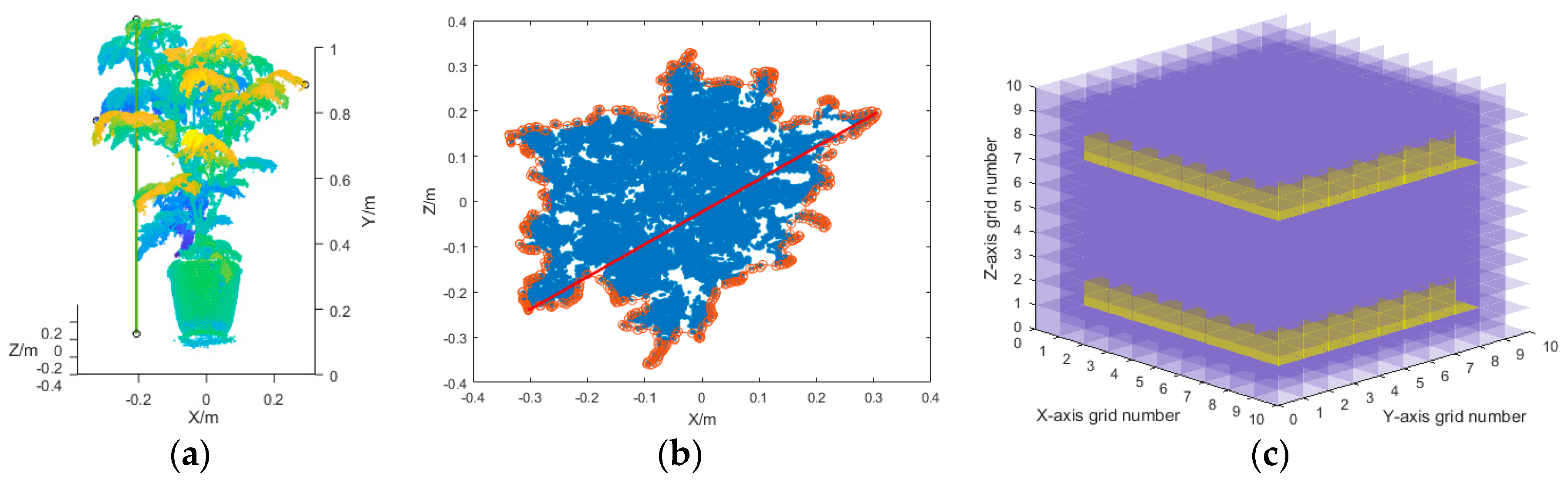
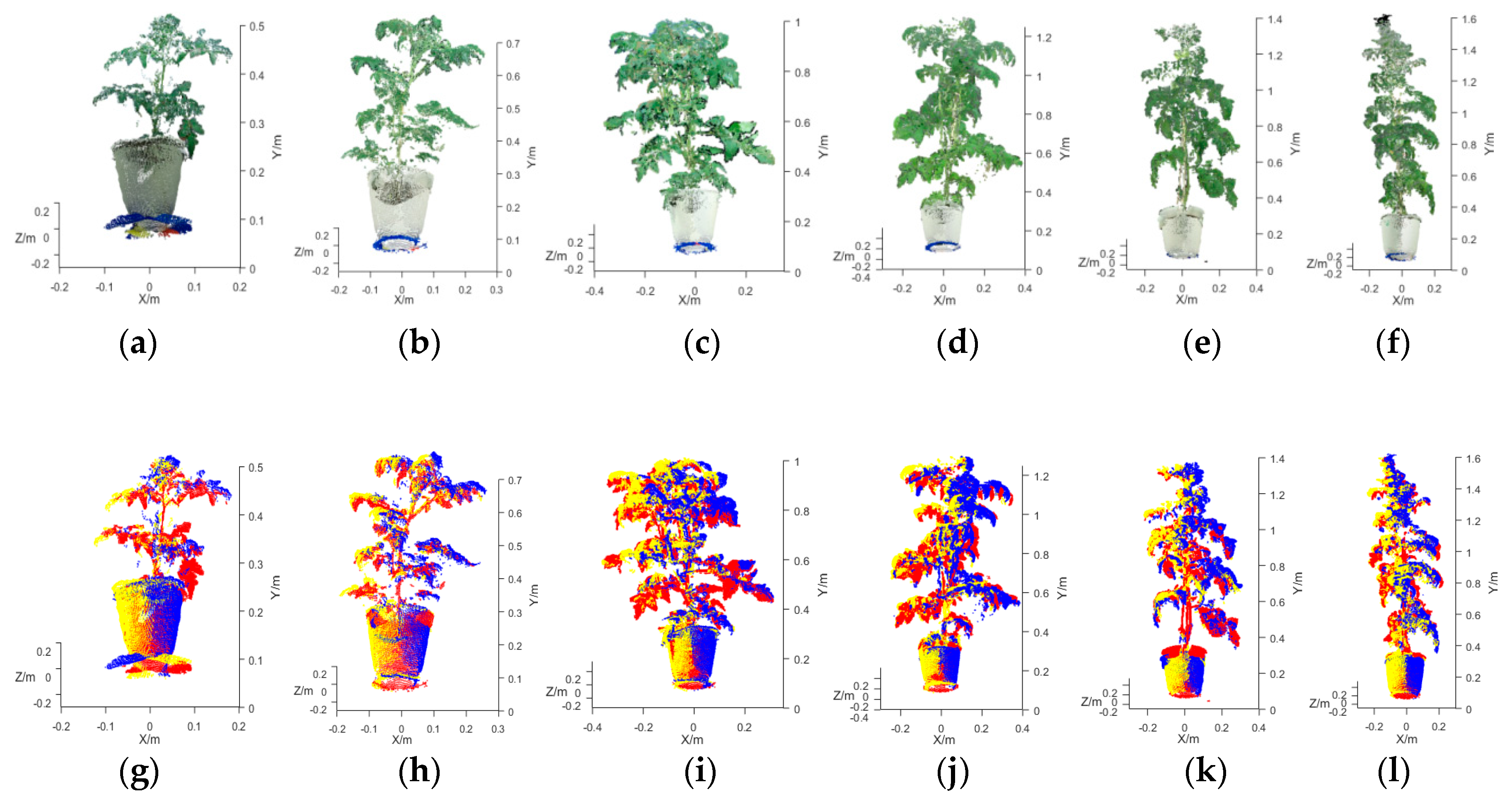
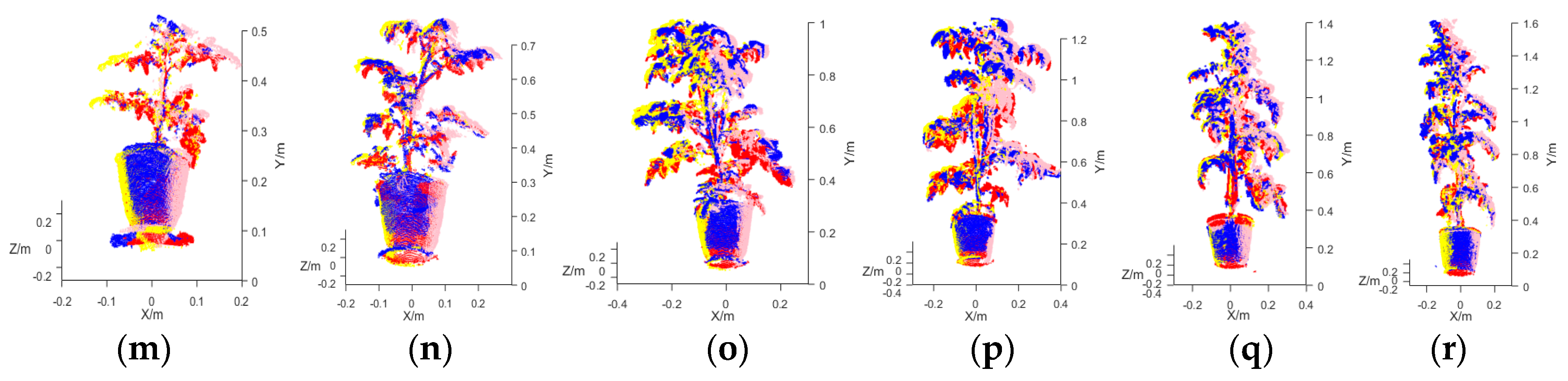
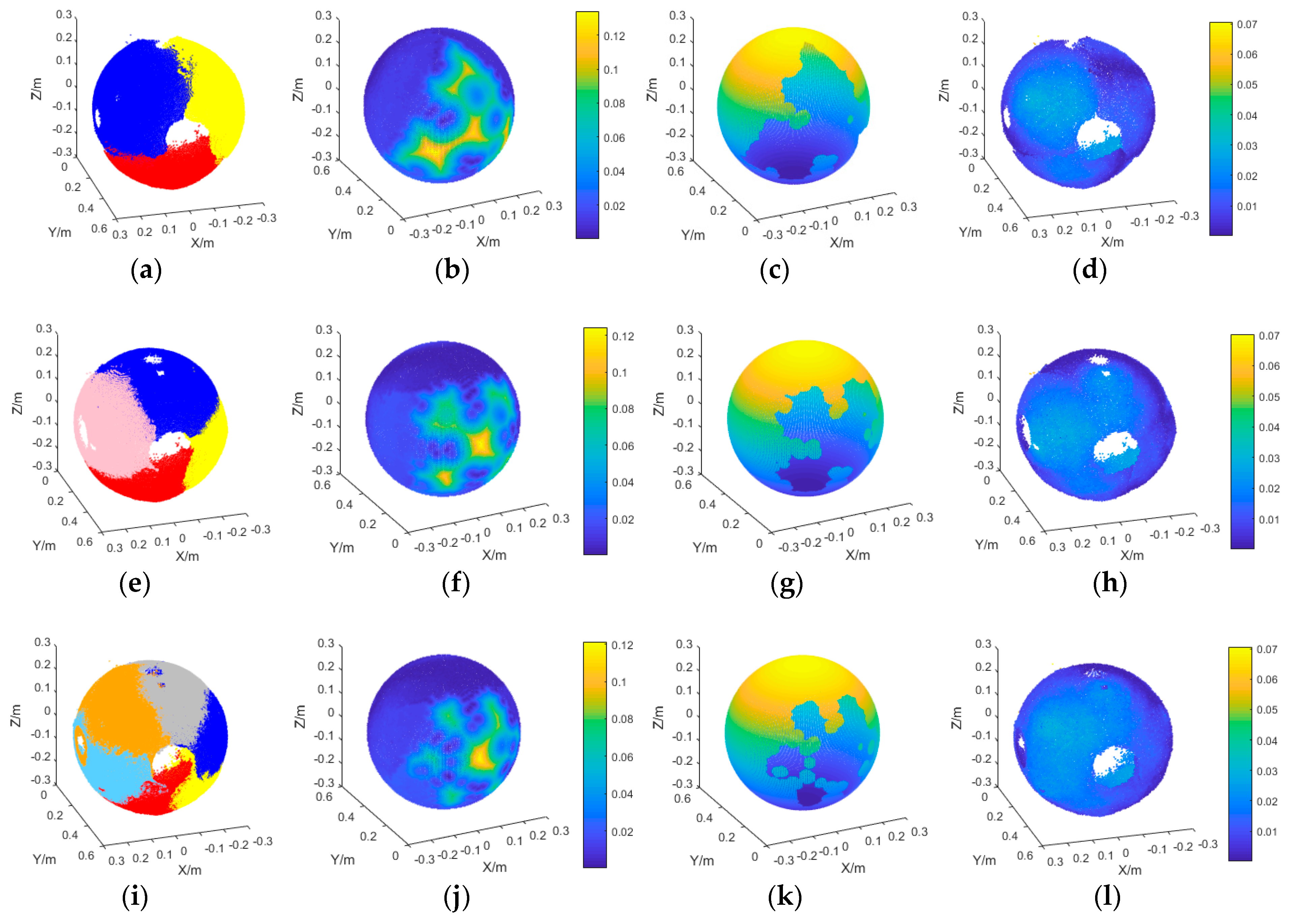
Figure A2 shows the reconstructed 3D point clouds of the SSB and corresponding reconstruction accuracy analysis.
Figure A2a shows the 3D point cloud of the SSB reconstructed based on RGB-D images captured at three AOVs (point clouds at 0°, 120°, and 240°, highlighted in red, yellow, and blue, respectively). The 3D point cloud was down-sampled using a 3D mesh filter. The 3D mesh threshold was set to 5 mm. Based on its outer boundary, the volume of the 3D point cloud of the SSB was calculated. As shown in
Figure A2b, a set of distances (
HSR) between the points of the reference and reconstructed point clouds of the SSB was calculated. When
HSR < 5.00% of the diameter of the SSB, the point was considered to have been scanned by the sensor. In
Figure A2c, the area of the SSB scanned by the sensor is marked. Based on Equation (6), the
Cr of the reconstructed point cloud was calculated. Based on Equations (7)–(10),
HD and
HRS of the SSB were calculated,
HRS as shown in
Figure A2d.
Figure A2.
Reconstructed 3D point cloud of the SSB and reconstruction accuracy analysis. (a) point cloud of the SSB reconstructed based on images captured at three AOVs, (b) HSR set, (c) area covered by the reconstructed point cloud, (d) HRS set. (a–d) Point clouds reconstructed based on images captured at three AOVs. (e–h) Point clouds reconstructed based on images captured at four AOVs. (i–l) Point clouds reconstructed based on images captured at six AOVs.
Similarly,
Figure A2e–h and
Figure A2i–l show the 3D point clouds of the SSB reconstructed based on images captured at four and six AOVs, respectively, as well as corresponding reconstruction accuracy analysis. In
Figure A2e, the four AOVs (0°, 90°, 180°, and 270°) are highlighted in red, yellow, blue, and gray, respectively. In
Figure A2i, the six AOVs (0°, 60°, 120°, 180°, 240°, and 300°) are highlighted in red, yellow, blue, gray, orange, and sky blue, respectively.
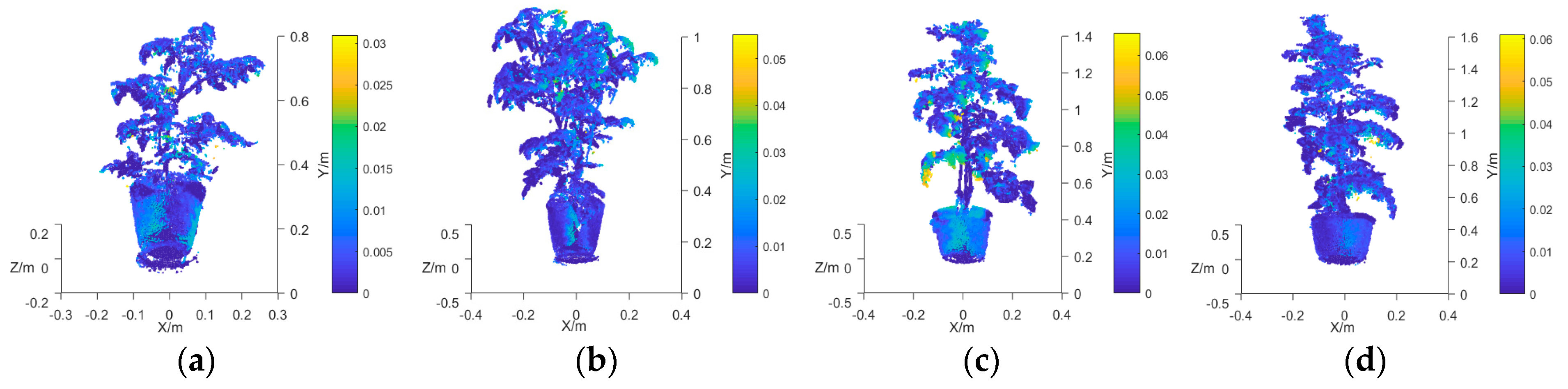
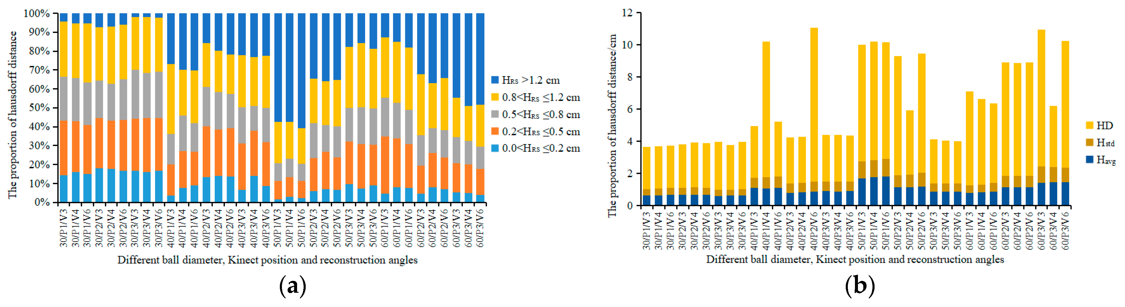
To quantitatively describe the accuracy of SSB 3D point cloud reconstruction, the distribution of the
HRS set of each of the SSBs with diameters of 30, 40, 50, and 60 cm and the corresponding point clouds reconstructed based on images captured by the Kinect sensor in three positions (
P1,
P2, and
P3) and at three, four, and six AOVs (
V3,
V4, and
V6) (a total of 36 combinations of measurement conditions) were statistically analyzed. The results are shown in
Figure A3a.
HRSs were categorized into five groups for statistical analysis, namely, 0 cm <
HRS ≤ 0.2 cm, 0.2 cm <
HRS ≤ 0.5 cm, 0.5 cm <
HRS ≤ 0.8 cm, 0.8 cm <
HRS ≤ 1.2 cm, and
HRS > 1.2 cm.
Figure A3.
Analysis of point cloud reconstruction of the SSBs: (a) Distribution of the HRS sets of the SSBs; (b) Metrics for assessing the accuracy of SSB 3D point cloud reconstruction.
Figure A3.
Analysis of point cloud reconstruction of the SSBs: (a) Distribution of the HRS sets of the SSBs; (b) Metrics for assessing the accuracy of SSB 3D point cloud reconstruction.
Figure A3b shows the metrics for assessing the accuracy of 3D point cloud reconstruction of SSBs, namely,
HD and the average (
Havg) and standard deviation (
Hstd) of the
HRS set. A comparison of the point clouds of the SSBs with diameters of 30, 40, 50, and 60 cm reconstructed based on images captured by the Kinect sensor in positions
P1,
P2, and
P3 at
V3,
V4, and
V6 and the corresponding respective reference point clouds shows that the average
HDs were 2.77, 4.33, 5.41, and 6.38 cm, respectively; the average
Havgs were 0.64, 0.93, 1.26, and 1.14 cm, respectively; the average relative
Havgs were 2.13%, 2.33%, 2.52%, and 1.90%, respectively; and the average
Hstds were 0.41, 0.64, 0.79, and 0.72 cm, respectively. The statistical data show that the excessively large
HDs were caused by the noise in the point clouds. However, based on
Havg and relative
Havg, the average distance between the reconstructed and reference point clouds of the SSBs was less than 1.26 cm, and the error in the reconstructed point clouds was less than 2.52%. A comparison of the point clouds of the SSBs reconstructed based on images captured at
V3,
V4, and
V6 and the corresponding reference point clouds shows that the average
HDs were 4.68, 4.38, and 5.12 cm, respectively; the average
Havgs were 0.98, 0.99, and 1.01 cm, respectively; and the average
Hstds were 0.62, 0.64, and 0.65 cm, respectively. A comparison of the point clouds of the SSBs reconstructed based on images captured by the Kinect sensor in positions
P1,
P2, and
P3 and the corresponding reference point clouds shows that the average
HDs were 5.26, 5.29, and 3.81 cm, respectively; the average
Havgs were 1.08, 0.95, and 0.95 cm, respectively; and the average
Hstds were 0.67, 0.64, and 0.61 cm, respectively. According to the statistical data, because
Cr varied insignificantly between
V3,
V4, and
V6 and the reconstructed point clouds were down-sampled in the same way, the accuracy of point cloud reconstruction was not significantly affected by
VN or by the Kinect sensor position.
Table A1 summarizes the statistical morphological measurement error data for the point clouds of the SSBs reconstructed based on images captured by the Kinect sensor in positions
P1,
P2, and
P3 and at
V3,
V4, and
V6. For the SSBs with diameters of 30, 40, 50, and 60 cm, the RADs for
DY were 2.96%, 2.49%, 1.99%, and 1.97%, respectively; the coefficients of variation (CVs) for
DY were 3.50%, 4.14%, 4.06%, and 4.76%, respectively; the RADs for
DX were 2.01%, 1.63%, 1.40%, and 1.61%, respectively; the CVs for
DX were 2.27%, 2.53%, 3.08%, and 4.42%, respectively; the RADs for
Vol were 4.87%, 3.95%, 1.72%, and 5.02%, respectively; the CVs for
Vol were 5.27%, 4.35%, 2.06%, and 5.18%, respectively; and the average
Crs were 92.81%, 89.85%, 89.91%, and 86.42%, respectively. The statistical data show that the measurement error in
DX was smaller than that in
DY and that the CV for
DX was smaller than that for
DY. This measurement error occurred mainly because some areas of the top and bottom of each SSB were not scanned, as shown in
Figure A2. In addition,
Cr decreased as the diameter of the SSB increased.
Table A1.
Analysis of morphological measurements of SSBs that differ in diameter.
Table A1.
Analysis of morphological measurements of SSBs that differ in diameter.
| Ball Diameter/cm | DY | DX | Vol | Cr/% |
|---|
| RAD/% | CV/% | RAD/% | CV/% | RAD/% | CV/% |
|---|
| 30 | 2.96 | 3.50 | 2.01 | 2.27 | 4.87 | 5.27 | 92.81 |
| 40 | 2.49 | 4.14 | 1.63 | 2.53 | 3.95 | 4.35 | 89.85 |
| 50 | 1.99 | 4.06 | 1.40 | 3.08 | 1.72 | 2.06 | 89.91 |
| 60 | 1.97 | 4.76 | 1.61 | 4.42 | 5.02 | 5.18 | 86.42 |
Table A2 summarizes the RADs for
DY,
DX, and
Vol and average
Cr of the point clouds of SSBs with diameters of 30, 40, 50, and 60 cm reconstructed based on images captured by the Kinect sensor in three positions (
P1,
P2, and
P3) and at three, four, and six AOVs (
V3,
V4, and
V6). For measurements taken at
V3,
V4, and
V6, the RADs for
DY were 2.33%, 2.38%, and 2.34%, respectively; the RADs for
DX were 1.52%, 1.42%, and 2.05%, respectively; the RADs for
Vol were 4.14%, 4.00%, and 3.52%, respectively; and the average
Crs were 85.45%, 90.17%, and 93.62%, respectively. The statistical data show that
VN did not significantly affect the error in the morphological measurement of the point cloud, but
Cr increased significantly as
VN increased. For measurements taken in positions
P1,
P2, and
P3, the RADs for
DY were 1.24%, 2.70%, and 3.12%, respectively; the RADs for
Dx were 1.30%, 1.31%, and 2.37%, respectively; the RADs for
Vol were 3.32%, 4.16%, and 4.19%, respectively; and the average
Crs were 87.10%, 87.60%, and 94.54%, respectively. The statistical data show that as the distance between the Kinect sensor and the measurement object decreased,
Cr increased significantly, but the RADs for the morphological parameters also increased.
Table A2.
Analysis of the morphological measurements of the SSBs (at various AOVs and in various positions).
Table A2.
Analysis of the morphological measurements of the SSBs (at various AOVs and in various positions).
| Reconstruction Angle | RAD | Cr | Kinect Position | RAD | Cr/% |
|---|
| DY/% | DX/% | Vol/% | DY/% | DX/% | Vol/% |
|---|
| V3 | 2.33 | 1.52 | 4.14 | 85.45 | P1 | 1.24 | 1.30 | 3.32 | 87.10 |
| V4 | 2.38 | 1.42 | 4.00 | 90.17 | P2 | 2.70 | 1.31 | 4.16 | 87.60 |
| V6 | 2.34 | 2.05 | 3.52 | 93.62 | P3 | 3.12 | 2.37 | 4.19 | 94.54 |
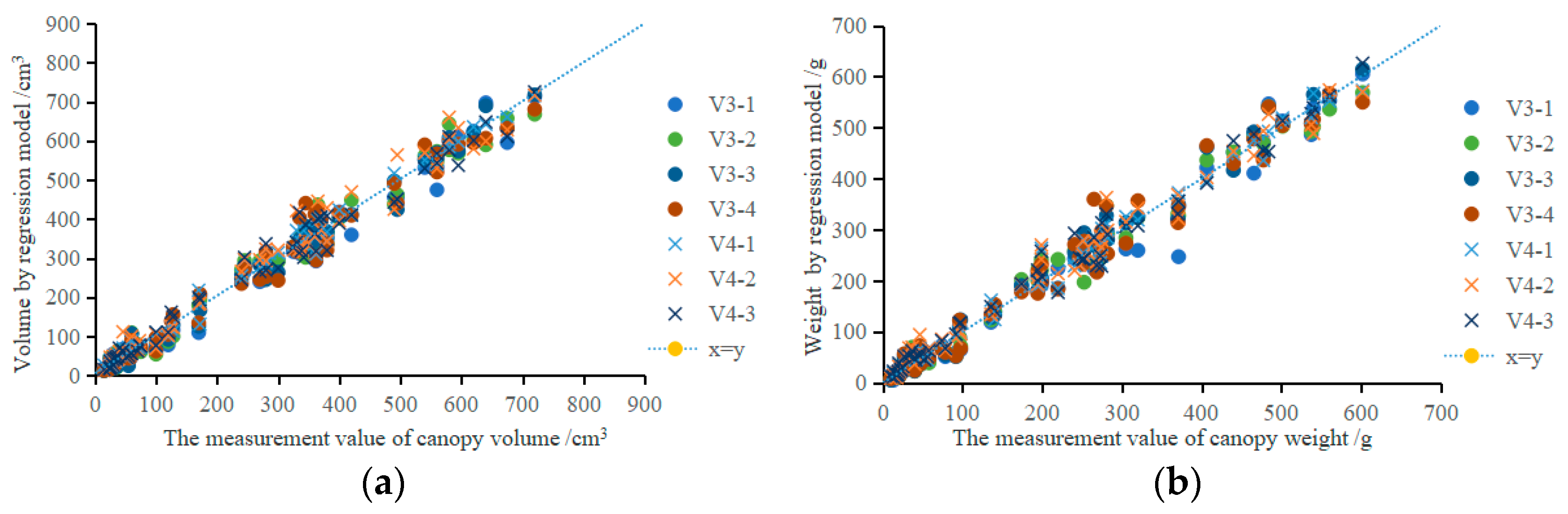
Based on the above analysis, for measurements taken at V3, V4, and V6, the average Crs were 85.45%, 90.17%, and 93.62%, respectively. The greater the number of perspectives, the greater the coverage, but the lower the reconstruction efficiency. Because the SSB is an entity measurement object, and the tomato plant is only partially blocked under each perspective, V3 and V4 reconstruction methods were selected to reconstruct the greenhouse tomato plants.


