Modelling Climate Suitability for Rainfed Maize Cultivation in Kenya Using a Maximum Entropy (MaxENT) Approach

Abstract

Climate change and variability are projected to alter the geographic suitability of lands for crop cultivation. In many developing countries, such as Kenya, information on the mean changes in climate is limited. Therefore, in this study, we model the current and future changes in areas suitable for rainfed maize production in the country using a maximum entropy (MaxENT) model. Maize is by far a major staple food crop in Kenya. We used maize occurrence location data and bioclimatic variables for two climatic scenarios-Representative Concentration Pathways (RCP) 4.5 and 8.5 from two general circulation models (HadGEM2-ES and CCSM4) for 2070. The study identified the annual mean temperature, annual precipitation and the mean temperature of the wettest quarter as the major variables that affect the distribution of maize. Simulation results indicate an average increase of unsuitable areas of between 1.9–3.9% and a decrease of moderately suitable areas of 14.6–17.5%. The change in the suitable areas is an increase of between 17–20% and in highly suitable areas of 9.6% under the climatic scenarios. The findings of this study are of utmost importance to the country as they present an opportunity for policy makers to develop appropriate adaptation and mitigation strategies required to sustain maize production under future climates.

1. Introduction

Climate change has become the greatest global challenge that is affecting cropping patterns and yields, leading to threats on food security for the growing population [1,2]. According to the Fifth Assessment Report of the Intergovernmental Panel on Climate Change (IPCC), climate change is likely to alter the distribution of crops in the world, leading to increased suitability of lands in Northern Hemisphere higher altitudes and decreased suitability in tropical regions [3]. For instance, in eastern Africa, suitability of lands for rainfed maize cultivation is likely to shift from lower to higher elevation regions under the A1F1 scenario [3]. Kenya, being one of the countries in this region, is no exception when it comes to the impacts of climate change on maize cultivation, which is a major staple food for over 90% of the population [4]. According to Zabel et al. [5], country specific estimates on the changes in land suitability for agricultural production under the changing climate are critical in order to develop adequate adaptation and mitigation strategies.

In the recent years, multiple modelling programs to analyse suitability for the production of crops under changing climate have been made possible by the current advances in remote sensing and geographic information techniques [6]. Alongside this, projections of climate variabilities have been broadly researched and reported based on general climate models (GCMs) [3]. The use of species distribution models (SDMs), which are regarded as empirical tools in ecology and natural resource management, has been accepted as important in generating predictions of the presence of species based on correlations between environmental variables and geo-localized species data [7]. Apart from delineating the necessary conditions for the species, SDMs predict spatial and temporal potential distribution of species [8,9]. Importantly, SDMs have been used to identify hotspots of threatened species, evaluate the possible hazard of invasive species and predict biodiversity and to establish potential locations for species cultivation in response to climate change [10,11,12,13].

Some of the SDMs that have been developed for this purpose include: dynamic simulation model (CLIMEX and BIOCLIM), generalized additive model (GAM); neural networks; generalized linear model (GLM); and Maximum Entropy (MaxENT) model [7,13,14,15,16]. Among the models, MaxENT is one of the widely used species distribution models to predict potential distribution of target species [14], for example, invasive species range dynamics [11,17], potential distribution of agricultural crops [18,19,20,21,22] and threatened forest species in the Philippines [23], among others.

According to Beck [24], there has been increased application of ecological niche models to investigate the impact of climate change on crop plants. However, despite the importance of maize being a staple food crop in Kenya, there is relatively limited documented information on future climatic suitability for maize production. As a step towards filling this research gap, the objective of the present study was to analyse the current and potential impacts of climate change on suitability of various parts of the country for maize cultivation using the Maximum Entropy (MaxENT) model. The specific objectives of the study were to: (1) select the climatic factors that potentially affect spatial suitability for maize production; (2) model the current and projected future suitability of lands based on two climate scenarios (RCP 4.5 and 8.5) for the year 2070; (3) examine suitability of lands for maize production in various counties; and (4) determine spatial climatic suitability shifts for maize production in the country. This study is essential, as the findings will provide basic information towards development of adaptation and mitigation strategies for maize production under the facets of climate change.

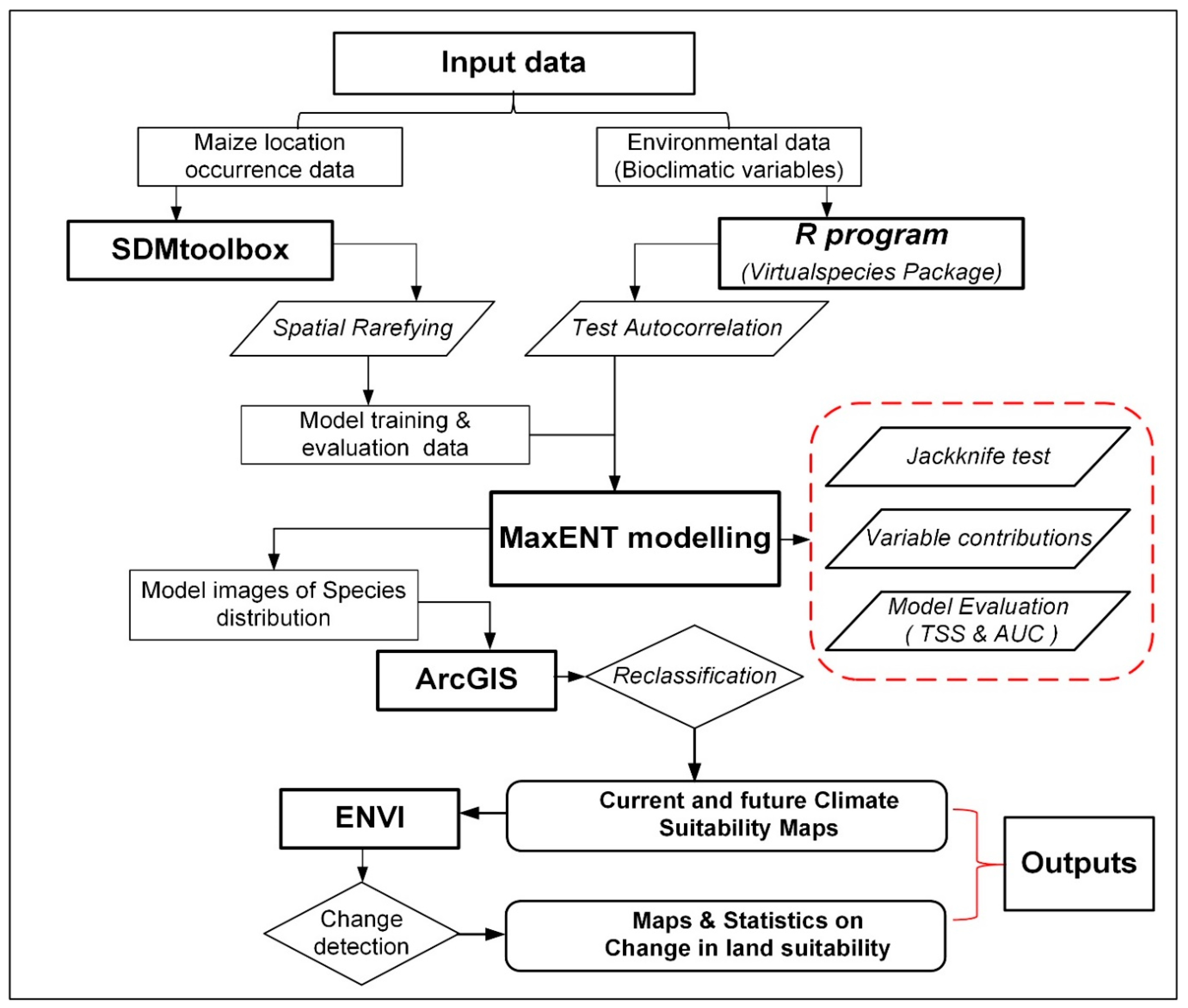
2. Materials and Methods

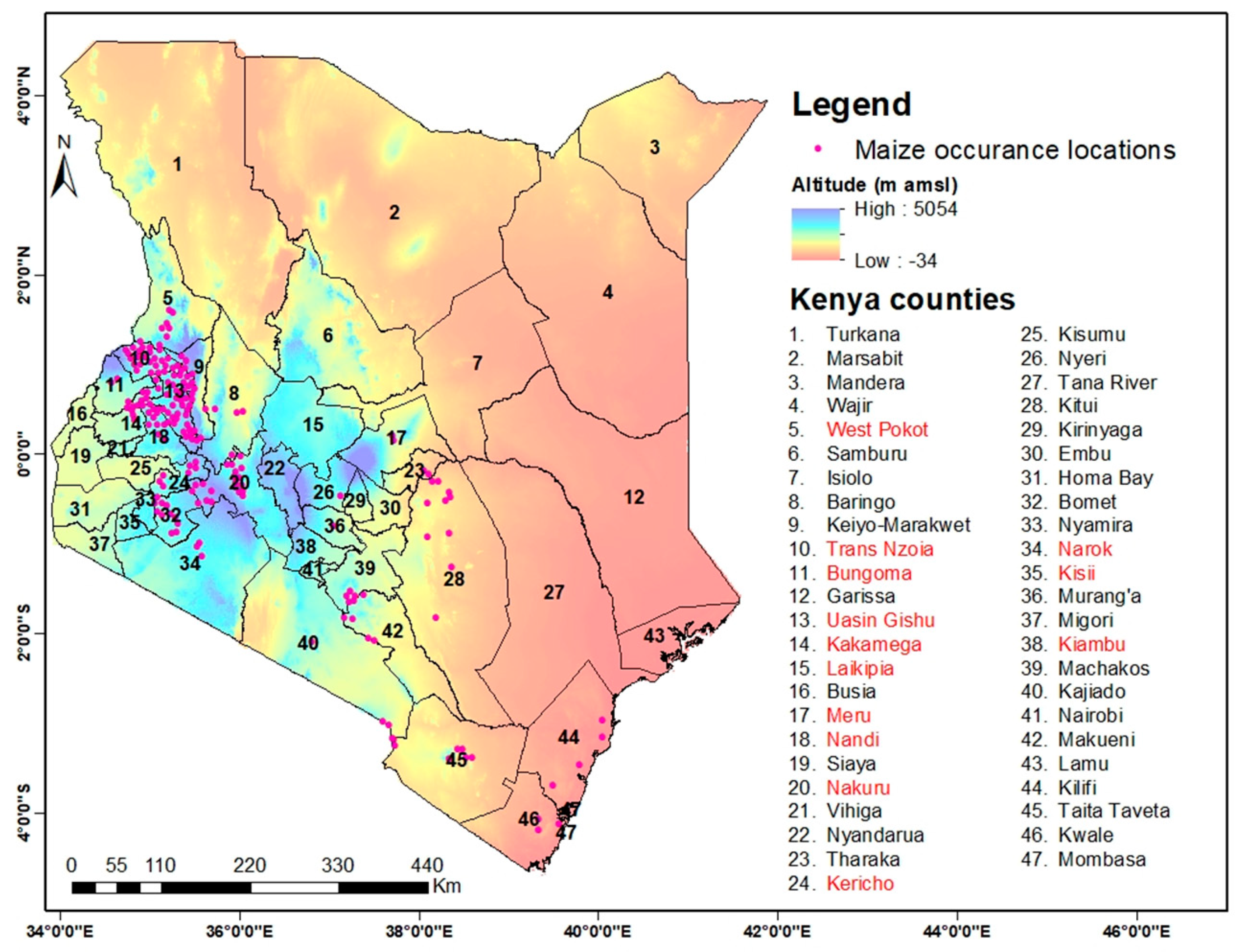
2.1. Study Area

This study focused on Kenya, which is divided into 47 administrative regions of counties and lies on latitude 5°S-5°N and between longitude 34°E-42°E (Figure 1). The country’s climate is moderated by variability in topography and the influence of the Indian Ocean and Lake Victoria. Temperatures range from 15 to 35 °C and have increased at an average rate of 0.21 °C per decade since 1960 and are projected to increase by 1.6 to 2.7 °C by 2060s [25]. The mean annual rainfall is bi-modal and ranges from 200 to 2200 mm. The long rains occur in the months of March to May, and the short rains from October to December. Approximately 84% of the country’s land area is either arid or semi-arid and only 16% falls between high and medium potential, suitable for crop production [26]. The agro-ecological zones in Kenya include: (I) low tropics; (II) dry mid; (III) moist-mid; (IV) dry transitional; (V) moist transitional; (VI) high transitional; and (VII) the arid zones [27]. Maize is Kenya’s major crop and is mainly grown in areas located in agro-ecological zones II- IV under rainfed conditions [28]. The major counties where maize is produced in Kenya are Trans-Nzoia, Uasin Gishu, Nandi, Nakuru, Laikipia, Kisii, Narok, Bungoma, Kakamega, Nandi, Kericho, Kiambu and Meru (Figure 2).

2.2. Environmental Modelling Data

The data used in this study were divided into bioclimatic and geographic distribution data of maize growing locations. The data on current bioclimatic information were obtained as raster layers from WorldClim [29] available at 30 arc-seconds (~1 km²) spatial resolution at the equator [30]. To predict the future area suitability for maize cultivation under climate change scenarios, the study used downscaled global climate model data from the Coupled Model Inter-Comparison Project Phase 5 (CMIP5) for the year 2070 under greenhouse gas (GHG) concentration scenarios (RCP 4.5 and 8.5) available on http://worldclim.org/cmip5_30s (accessed February, 2019) [30]. Among the GCMs available, we used the Hadley Centre Global Environmental Model 2-Earth System (HadGEM2-ES) and the Community Climate System Model, Version 4 (CCSM4). Our use of HadGEM2-ES was motivated by the work of Dike et al. [31], who observed that the model simulations were close to the multimodel ensemble mean over Africa. Likewise, CCSM4 has improved El Niño-Southern Oscillation (ENSO) variability with more reasonable frequency distribution compared to earlier versions of CCSMs [32]. ENSO is a major driver of interannual rainfall variability in eastern Africa [33].

Data were retrieved for RCP 4.5 and RCP 8.5, which represent medium and high emissions scenarios, respectively [3]. A multicollinearity test was undertaken using R-program Package ‘virtualspecies’ (version 1.4–4) to screen highly correlated environmental predictors among the 19 bioclimatic variables that represent a combination of annual trends, extreme environmental conditions and seasonality. In recent SDM literature, this package has been used for variable selection [17]. The temperature-related variables include the annual mean temperature (BIO₁), diurnal temperature range (BIO₂), Isothermality (BIO₃), temperature seasonality (BIO₄), maximum temperature of warmest month (BIO₅), minimum temperature of the coldest month (BIO₆), annual temperature range (BIO₇), mean temperature of the wettest quarter (BIO₈), mean temperature of the driest quarter (BIO₉), mean temperature of the warmest quarter (BIO₁₀), and the mean temperature of the coldest quarter (BIO_11). The precipitation-related bioclimatic variables include annual precipitation (BIO₁₂), precipitation of the wettest month (BIO_13A), precipitation of the driest month (BIO₁₄), precipitation seasonality (BIO₁₅), precipitation of the wettest quarter (BIO₁₆), precipitation of the driest quarter (BIO₁₇), precipitation of the warmest quarter (BIO₁₈) and precipitation of the coldest quarter (BIO₁₉) (http://worldclim.org/bioclim). A Pearson correlation coefficient (r) ≥ 0.7 was selected as an absolute value to filter out correlated variables as it has been recognized as an acceptable threshold level to minimize multicollinearity [34] (Figure S1). Some variables under the same cluster were selected due to their importance in maize productivity. Thus, a subset of seven variables was selected for model runs (Table S1). All the bioclimatic variables were converted into Raster ASCII GRIDS (.asc) format that is acceptable by the MaxENT model and projected to WGS1984_UTM_Zone37N. Finally, spatial jackknifing tests were performed for the selected variables using the SDMtoolbox to ascertain the relative contributions of each of the variables to the MaxENT model [35]. As per Phillips et al. [36], the Jackknifing procedure is one of the in-built functions of MaxENT that operates by excluding each variable in turn and creating a model with the remaining variables, creating a new model using each variable in isolation.

2.3. Species Occurrence Data

As per the FAO database, the average land area under maize production in Kenya between the years 2000 to 2017 was 1,871,147 hectares [37]. The farms where maize is grown were visually identified by systematically scanning maize growing counties in Google Earth, based on the first author’s knowledge of maize farms in the country. The maize farms could easily be identified visually in satellite images based on the distinct growing pattern and coloration of vegetation. Through this process, 962 occurrence points (Table S2) were extracted from the identified maize farms in various counties and their coordinates recorded for use in the model. Considering that there are a number of counties with zero maize production, we selected most occurrence points from farms in the western part of Kenya, which has diversified agro-ecological zones in order to capture variability. We compared the geographic coordinates of the locations on the map of Kenya croplands [38] (Figure S2). Considering that some of the points were close to each other, we used spatial rarefaction in the SDMtoolbox of ArcGIS (version 10.4.1) at a maximum user distance of 10 km in order to eliminate multiple auto correlated occurrence locations [35,36,39]. Through this process, the output was a record of 295 farms that were finally used as training data in the model (Figure 2).

2.4. Ecological Niche Modelling

In this study, we used Maximum Entropy software (MaxENT version 3.4) [36,40] to analyse current and future shifts in lands suitable for the cultivation of Zea mays L. in Kenya. Among the SDMs, we chose MaxENT based on the following reported advantages: (i) it is considered the best available species distribution and is highly regarded due to its superlative analytical capacity and precision in predicting distribution of different floral species [14]; (ii) the model performance is good with presence-only data and small numbers of records, and can utilize both continuous and categorical variables [23,36]; (iii) it is resistant to spatial errors in occurrence data to some extent and performs well with occurrences that show sampling bias [41]. The model computes the likely distribution of a species with the support of maximum entropy rules and statistical mechanisms [36]. The predictors that the model mainly utilizes are the environmental variables and the species occurrence information. The idea of MaxENT is to use species presence-only data and a set of environmental predictors across a defined land scape to compute the probability of target distribution by finding the possibility of maximum entropy [36]. The MaxENT algorithm builds on subjecting the constraints on an unknown target probability distribution over a set of known features (denoted as J, which in our case are the environmental variables or predictors thereof). For each site x_i, a non-negative probability denoted as p is assigned, and the likelihood is assumed to sum to 1. According to Phillips et al. [36], the entropy estimate of $\hat{\mathsf{\pi }}$ is defined as:

$$H \left(\hat{\mathsf{\pi }}\right)=-{{\displaystyle \sum }}_{x\in X}\hat{\mathsf{\pi }}\left(x\right)ln\hat{\mathsf{\pi }}\left(x\right)$$

(1)

where ln is the natural logarithm.

As per Merow et al. [42], the relative occurrence rate (ROR) is predicted by MaxENT as a function of predictors at a particular location that is defined in the form:

$$ROR=\exp (\mathrm{z}\left({\mathrm{x}}_i\right)|/{{\displaystyle \sum }}_i\exp \mathrm{z}\left({\mathrm{x}}_i\right)|)$$

(2)

where z is a vector of J environmental variables at location x_i, and | denotes a vector of regression coefficients.

2.5. MaxEnt Settings and Evaluation of Model Accuracy

The model was set to use 80% of the 295 maize presence locations as predictive training samples, and the remaining 20% for performance testing. The sub-sampling technique of the MaxENT algorithm was used and the model set to 10 replicates in order to use all the data efficiently and to ensure a more realistic average output [36]. This also helps to evaluate uncertainty in the model [42]. For model convergence, the number of maximum iterations was set to 5,000 in order to attain adequate predictions [36]. The number of background points for each analysis was set to 10,000 to represent pseudo-absence locations which are used by the model to define probability distribution and estimates [43]. Overall validation of the model was evaluated using the threshold-dependent True Skill Statistics (TSS) and threshold-independent area under the curve (AUC) of the receiver-operating characteristic (ROC) which is a plot of sensitivity against specificity [36,44]. According to Allouche et al. [45], TSS takes into account both the omission and commission errors and success as a result of random guessing and is presented as:

$$TSS=Se+Sp-1$$

(3)

where Se is the sensitivity and Sp is the specificity. As per Mason and Graham [46], AUC is determined as follows:

$$AUC=\frac{1}{n_1{n}_0}{\displaystyle \sum }_{i=1}^{n_1}{\displaystyle \sum }_{j=1}^{n_0}I\left(x_{1i},x_{0j}\right)$$

(4)

where

$$I\left(x_{1i} ,x_{0j}\right)=\{\begin{array}{ccc}0& if& x_{1i}< x_{0j}\\ 0.5& if& x_{1i}=x_{0j}\\ 1& if& x_{1i}>x_{0j}\end{array}$$

(5)

and where $x_{1i}$ is the predicted value for the presence site denoted as $n_1,$ and $x_{0j}$ is the predicted value for absence site denoted as $n_0$.

2.6. Reclassification and Change Detection

First, the simulated MaxENT outputs that present the possibility of a given geographic area for maize production was reclassified using the natural breaks (Jenks) classification method in ArcGIS. The classes of suitability under this study are described in

Table 1. Suitability assessment for maize cultivation in Kenya.

Class of Suitability	Suitability Cut-Off Values	Description
Highly suitable	>0.8	Lands with optimal conditions suitable for maize cultivation
Suitable	0.6–0.8	Lands with minor climatic limitations for optimal maize cultivation
Moderately suitable	0.2–0.4	Land with major climatic limitations that may significantly reduce production of maize
Unsuitable	<0.2	Lands with severe climatic limitations that are not favourable for cultivation of maize

:

Secondly, change detection was undertaken through an overlay analysis in ENVI (version 5.5) with the aim of analysing the spatial shifts in land from current to projected suitability under the various climate scenarios for the year 2070. The nature of the spatial shifts in the land suitability classes described in Table 1 was identified as follows: (1) expansion due to a gain from the conversion of other land categories; (2) Improvement due to a shift of a given land class to better suitability conditions; (3) Reduced suitability due to a conversion to a lower suitable category; (4) Constant/unchanged when the land areas remain under the same suitability category under the present and future climate.

Figure 3 is a methodological flowchart summarizing the above methodology. Presented are the inputs, data processing pathways and tools, MaxEnt modelling outputs and final processes of preparation of outputs and analysis through change detection.

3. Results

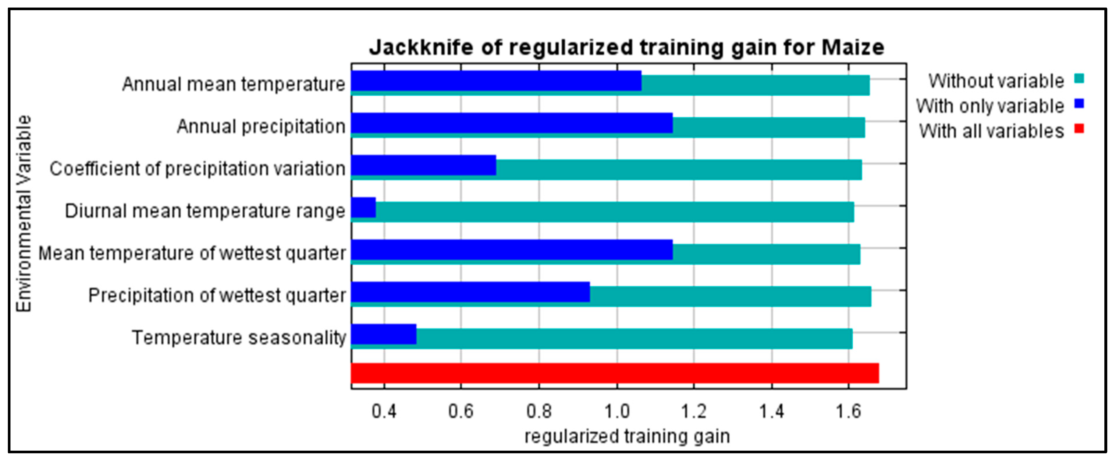
3.1. Climatic Variables Influencing Land Suitability for Maize Cultivation

The climatic factors that affect area suitability for maize production were derived from seven bioclimatic variables selected from each set of highly correlated predictors (Figure 4). The contribution of each of these predictors in influencing the geographic suitability for maize cultivation was analysed in a histogram of the jackknife test, which is one of the outputs of the MaxENT model.

As per the results of the jackknife test (Figure 4), it is important to note that the contribution of mean temperature of the wettest quarter, the annual rainfall and annual mean temperature are some of the predictors that present the most useful information in determining suitability of an area for maize cultivation (Figure 4). The percentage contributions of the bioclimatic predictors are presented in

Table 2. Contribution of bioclimatic factors that affect maize cultivation in Kenya.

Variable	Percentage Contribution (%)	Cumulative Contribution (%)
Annual precipitation	43.1	43.1
Mean temperature of the wettest quarter	31.2	74.3
Diurnal mean temperature range	9.5	83.8
Precipitation of the wettest quarter	6.7	90.5
Temperature seasonality	4.2	94.7
Coefficient of precipitation variation	3.4	98.1
Annual mean temperature	1.8	99.9

. The annual precipitation was the major determinant and contributed 43.1% to the model, followed by the mean temperature of wettest quarter at 31.2%. The lowest contributor was annual mean temperature. The accumulated percentage contribution of the seven variables was 99.9%.

3.2. Model Performance

In this study, the performance of the MaxENT model was examined based on the receiver operating characteristic curve (Figure 5) and TSS. The average AUC and TSS values for the 20% of the occurrence data for the ten replicate runs were 0.93 and 0.71, respectively.

3.3. Suitability Zones for Maize Production

Habitat suitability maps were created for the current and future regions for maize production and the coverage in Kenya (Figure 6 and Figure 7). Across the country, the simulation output shows that 70% of land is unsuitable for maize production under the present and future climate projections. The major counties that are not suitable are Marsabit, Turkana, Wajir, Garissa, Tana river, Mandera, Isiolo Kitui Samburu, Taita Taveta, Kilifi, Kajiado, Kwale, Lamu, Baringo, Meru, West Pokot, Makueni, Homa Bay and Siaya. The moderately suitable areas occupy between 16 and 19.6% of the country (Figure 6). The major counties that fall under this category are Nairobi, Machakos, Kiambu, Narok, Laikipia, Kajiado, Murang’a, Makueni, Nyeri, Vihiga, Embu, Nyandarua. At present, the highly suitable areas are estimated to occupy approximately 3.6% of the country and are projected to reduce in coverage to an average of 3.3% under RCP 4.5 and increase to an average of 4% under RCP 8.5. The counties in this category are Uasin Gishu, Trans Nzoia, Nandi, Nakuru, Baringo, West Pokot, Kericho, Keiyo-marakwet, Bungoma, Kakamega, Bomet, Kitui, Laikipia, Nyeri.

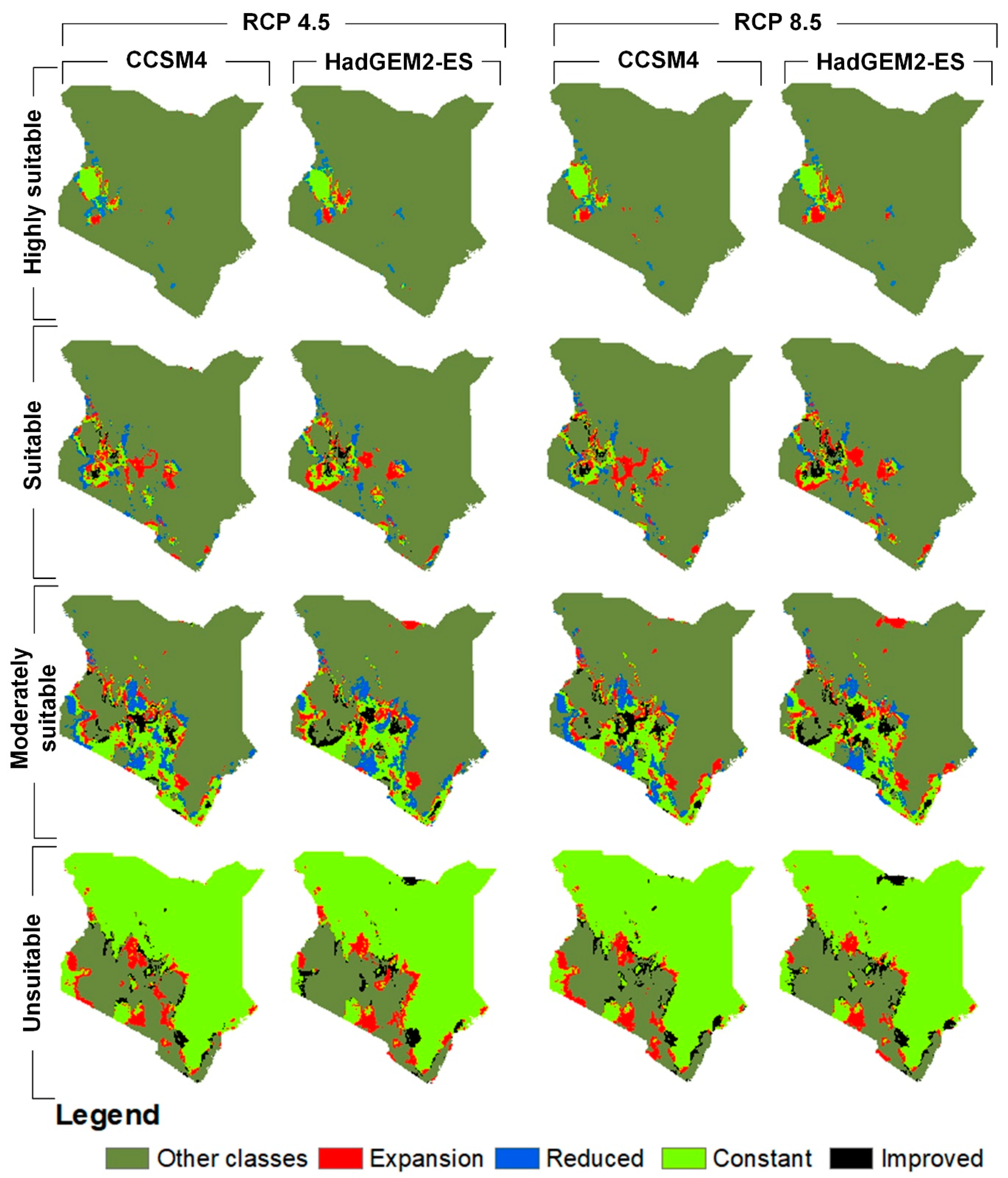
3.4. Change in Suitability for Maize Production

The predicted average conversions of the country’s suitability zones for maize production based on the two GCMs are presented in

Table 3. Changes in land suitability for maize production under RCP 4.5 in Kenya for 2070 compared to current suitability.

	Class of Suitability	Conversions from Current Climate in km2 (Percentage is Shown in Parentheses)				Area under (RCP 4.5)
		Unsuitable	Moderately Suitable	Suitable	Highly Suitable
RCP 4.5	Unsuitable	394,554 (95.8%)	31,262 (27.4%)	1931 (5%)	67 (0.3%)	427,814
	Moderately Suitable	16,704 (4.1%)	66,653 (58.4%)	10,062 (29%)	676 (3.2%)	94,094
	Suitable	608 (0.1%)	15,616 (13.7%)	19,084 (54%)	5,980 (28.3%)	41,288
	Highly suitable		558 (0.5%)	4,146 (12%)	14,395 (68.2%)	19,100
Total area (current)		411,865	114,089	35,223	21,118
Average change		15,987 (3.9%)	−19,936 (−17.5%)	6,065 (17%)	−2,019 (−6%)

Note: The average change represents the change in the class of suitability from the current climate.

and

Table 4. Changes in land suitability for maize production under RCP 8.5 in Kenya for 2070 compared to current suitability.

	Category Suitability	Conversions from Current Climate km2 (Percentage is Shown in Parentheses)				Area under (RCP 8.5)
		Unsuitable	Moderately Suitable	Suitable	Highly suitable
RCP 8.5	Unsuitable	391,033 (94.9%)	27,310 (23.9%)	1370 (4%)	3 (0.0%)	419,716
	Moderately Suitable	19,996 (4.9%)	67,198 (58.9%)	9502 (27%)	617 (2.9%)	97,313
	Suitable	836 (0.2%)	18,683 (16.4%)	17,954 (51%)	4643 (22.0%)	42,116
	Highly suitable	1 (0.0%)	898 (0.8%)	6397 (18%)	15,856 (75.1%)	23,152
Total area (current)		411,865	114,089	35,223	21,118
Average change		7877 (1.9%)	−16,707 (−14.6%)	6893 (20%)	2034 (9.6%)

. Projections for the future climate indicate that approximately 95% and 58.5% of the land will remain unsuitable and moderately suitable for maize production, respectively. Likewise, over 50% of suitable and 68–75% of highly suitable areas will remain unchanged. In terms of the changes in land suitability, it is projected that the climate will become unsuitable for the presently cultivated maize cultivars in parts of the currently moderately suitable lands in parts of Kajiado, Taita Taveta, Laikipia, Samburu, Narok, Kitui, Turkana and Siaya counties. This change is likely to cause expansion of unsuitable lands by an average of 27,310–31,262 km². However, parts of Marsabit, Lamu, Isiolo, Kitui and Meru counties that are currently unsuitable will shift to a moderately suitable status, by a total of 16,704 km² under RCP 4.5 and 19,996 km² under RCP 8.5. Likewise, 608–836 km² of the unsuitable land will be suitable for maize production.

The moderately suitable zones across Kenya are likely to reduce in coverage by approximately 19,936 km² (17.5%) and 16,707 km² (14.6%) under RCP 4.5 and RCP 8.5, respectively. The change in this category is as a result of predicted conversion to unsuitable zones by a total of 22,398 to 32,223 km². In addition, it is anticipated that there will be an improvement in the currently moderately suitable zones to better suitability by a total of between 16,174 to 19,581 km² that will majorly result from conversions in parts of Kajiado, Narok, Kitui, Embu, Machakos, Laikipia, Kwale and Kilifi counties. The suitable zones will increase by 22,203-24,162 km² under the projected climate through gains from deterioration of highly suitable lands and improvement in unsuitable and moderately suitable lands. It is projected that there be will an improvement in these zones due to conversion to highly suitable zones by a total of 4146–6397 km², mostly in parts of Nakuru, Baringo, Bomet, Kericho, Keiyo-Marakwet and Laikipia counties. The projected change in the highly suitable areas is a decrease in suitability of 5262–6732 km² and an expansion of an average of 4,704 km² under RCP 4.5 and 7296 under RCP 8.5.

The quantitative changes and maps of various suitability categories under the two IPCC scenarios, and HadGEM2-ES and CCSM4 GCMs presented in terms of improved suitability, unchanged/constant, expansion and decrease coverage are shown in

Table 5. Changes in land suitability categories.

Category of change	Change type	Area (km2) under RCP 4.5		Area (km2) under RCP 8.5
		CCSM4	HadGEM2-ES	CCSM4	HadGEM2-ES
Highly suitable	Constant	14,185 (67.2%)	14,606 (69.2%)	15,672 (74.2%)	16,039 (75.9%)
	Expand	4279 (20.3%)	5130 (24.3%)	5700 (27.0%)	8892 (42.1%)
	Decrease	6,933 (32.8%)	6512 (30.8%)	5446 (25.8%)	5079 (24.1%)
Suitable	Constant	18,513 (52.6%)	19,656 (55.8%)	18,375 (52.2%)	17,532 (49.8%)
	Expand	21,112 (59.9%)	23,294 (66.1%)	22,297 (63.3%)	26,027 (73.9%)
	Improve	3879 (11.0%)	4413 (12.5%)	5096 (14.5%)	7697 (21.9%)
	Decrease	12,831 (36.4%)	11,154 (31.7%)	11,752 (33.4%)	9994 (28.4%)
Moderately suitable	Constant	68,007(59.6%)	65,299 (57.2%)	64,882 (56.9%)	69,514 (60.9%)
	Expand	27,027(23.7%)	27,855 (24.4%)	28,976 (25.4%)	31,254 (27.4%)
	Improve	14,562 (12.8%)	17,786 (15.6%)	16,985 (14.9%)	22,178 (19.4%)
	Decrease	31,520 (27.6%)	31,004 (27.2%)	32,223 (28.2%)	22,398 (19.6%)
Unsuitable	Constant	396,188 (96.2%)	392,920 (95.4%)	392,854 (95.4%)	389,212 (94.5%)
	Expand	32,985 (8.0%)	33,536 (8.1%)	33,540 (8.1%)	23,827 (5.8%)
	Improve	15,677 (3.8%)	18,946 (4.6%)	19,012 (4.6%)	22,654 (5.5%)

Note: The percentages in parentheses denote the portion of the change in relation to the current suitability.

and Figure 8. Simulated results of areas under each climate suitability class for current and future maize production in various counties are presented in the Tables S3–S7).

4. Discussion

Geographic suitability of a given species is influenced by climatic variables that play a key role in the biological processes of the species growth, and this is critical in modelling [15,47]. This study investigated the current and potential geographic distribution of maize in Kenya for RCP4.5 and RCP8.5 scenarios using bioclimatic variables from HadGEM2-ES and CCSM4 GCMs. HadGEM2-ES used in this study was motivated by the findings of a study by Dike et al. [31], who observed that the model presents annual cycles of temperature and precipitation that are very close to the mean of CMIP5 models in Africa, thus, suitable for analysis of spatial patterns and future projections over the continent. The results from CCSM4 showed minor differences with those of HadGEM2-ES, which is contrary to the findings of Klein et al. [48], who indicated that the GCM does poorly in reproducing rainy seasons in East Africa. The minor variations in climatic suitability projections by the two models could be attributed to local differences in magnitudes of bioclimatic parameters as projected by the models and the RCPs.

The numbers of climatic variables were reduced from the initial 19 to seven variables (Figure 4) that have low correlation and are based on climate indices that have been used to examine maize production in Kenya and other regions in the world, such as the studies of Zhang et al. [6], He and Zhou [18], Mati [28], Ogutu et al. [49], Olson et al. [50]. The use of elevation was not considered since it is a proxy variable that could result in autocorrelations with temperature and rainfall data; bioclimatic variables are strong enough to determine the spatial limits of climatic tolerance of species [51,52].

In terms of model performance, the simulated results indicated that the average area under the curve (AUC) of the MaxENT model was 0.938, indicating good predictive accuracy [53,54,55]. The AUC value, which is closer to one, is indicative of minimum omission and commission errors of the model. The TSS value of the study was 0.71, which falls under the category of 0.4–0.8 that is considered as moderate performance [56] but towards the upper end. The Cohen’s kappa statistic, which is also used to measure model performance, was not used due to its dependency on prevalence [45]. In addition, the model jackknife test provided a measure on the contribution of the various environmental variables in influencing the suitability for maize production. The performance of the MaxEnt model confirmed its appropriateness for predicting climate suitability for maize production. This is in agreement with the findings of related studies that found the model is applicable in assessing crop suitability. Examples are studies on rice by Duan and Zhou [20] and Liu et al. [21]; maize by Machovina and Feeley [57], Ji et al. [58] and He and Zhou [18]; and banana by Machovina and Feeley [57]. This then confirms MaxENT’s capacity, which is based on machine learning and the principle of maximum entropy in estimating the multivariate distribution of habitat suitability conditions for crop suitability.

The results revealed that the annual temperature, mean annual precipitation and the mean temperature of the wettest quarter were the major factors influencing suitability for maize cultivation (Table 2). As for these contributors, it is worth understanding that the temperature governs maize suitability since it is a thermophilic C4 crop. For instance, temperature affects germination, growth and development of the crop. Similarly, annual precipitation plays a key role in water balances for growth and production of the crop [18,59,60].

Generally, different regions assume certain levels of suitability based on the changes in environmental parameters [61]. Therefore, any deviation of these parameters causes an improvement, an increase or decrease in the state of suitability for cultivation of a crop. In Kenya, maize usually does well in wetter areas than in drier regions because the most limiting factors are rainfall amount and distribution [28]. In addition, an increase in the suitability of high altitude areas for maize production will be directly related to an increase in temperature, but at lower elevations, the influential factor would be water balances [60].

Based on the climatic factors and the results of the MaxENT model, the geographic suitability of the climate for maize production in the country can be divided into highly suitable, suitable, moderately suitable and unsuitable areas, which at the present, almost match the distribution of maize cultivation in Kenya. For the current distribution, our simulation shows that the unsuitable areas occupy approximately 70.7% of the country and mainly cover the arid and semi-arid areas. The moderately suitable area covers approximately 19.6%, suitable being 6% and highly suitable areas being 3.6% (Table 3). These results are assumed to be acceptable due to the good performance of the model and the agreement of the findings with the present maize farming areas that fall under agro-climatic zones II, III and IV with rainfall of between 750 mm to 2200 mm per annum [28].

Due to impacts of climate change, the predicted future suitability of lands in Kenya is likely to result in some areas remaining constant, others expanding, improving or deteriorating in their suitability (Figure 7). From the findings, the extent of the unsuitable areas will increase by 2–4%, the moderately suitable areas are likely to decrease by 15–17% and the suitable areas likely to increase by 17–20% depending on the climate scenario. Likewise, the highly suitable areas are likely to decrease by 9.6% under RCP 4.5 or increase by approximately the same amount under RCP 8.5 (Table 4).

In terms of conversions in land suitability classes (Table 5), the simulation results show a higher likelihood of moderately suitable zones converting to unsuitable zones (27.4% under RCP 4.5 and 23.9% under RCP 8.5). Likewise, there is a potential shift of suitable lands of between 27–29% to moderately suitable lands. These conversions demonstrate a greater decrease in suitable areas compared to those that improve in suitability under both scenarios. As such, these findings seem to provide a more consistent picture, similar to the findings of Mati [28], who predicted a potential decrease of maize yields in zone III and an increase in zone IV agro-ecological zones of Kenya. Similarly, the findings strongly confirm the observations of the Fifth Assessment Report of the IPCC on the potential changes in agro-climatic zones [3]. For instance, the report predicts a possibility of shifts in agro-climatic zones that are currently good for crop production to more suitable and those that are currently marginally suitable becoming unsuitable [3].

The changes in suitability of lands for maize production in Kenya present an opportunity for the establishment of mitigation and adaptation measures required to sustain maize production under future climate. For instance, the government should consider taking advantage of the counties that are likely to experience potential expansion or improved suitability and explore their possibilities for future maize production. For the suitable and highly suitable areas that are likely to remain stable, it would be necessary to continue supporting and improving techniques for optimum maize production. However, in areas where there is potential decrease in suitability for maize production, there will be need to explore adaptation options such as potential alternative crops or shifts in diets in order to offset food shortages [62]. Other possibilities to counteract the negative impacts of climate change would be the use of irrigation and maize varieties with greater tolerance to local abiotic stresses and resistance to pests and diseases that may result from climate change [61,63].

Like most modelling studies on the effects of climate change on crop production, this study comes with some limitations. For example, there are substantial uncertainties in data on maize locations across the climate suitability classes and thus a constraint to notably examine the actual impacts on maize cultivation. Secondly, visual selection of occurrence location points may cause substantial bias in sample selection. In addition, we have not taken into consideration the influence of edaphic factors that affect the land on which particular crops grow, such as maize in this case. Soil is a medium in which the plant grows and supplies moisture and nutrients required for development and climate change is projected to significantly affect its processes and composition [6]. However, information on the contribution of soil to suitability of lands for crop production under a future climate has not been developed for Kenya. Other limitations include the influence of non-climatic factors such as changes in land uses, which could be considered in future research to further improve the results. We have also used a one niche modelling method (MaxENT) whose results may be different from those of other models. However, other studies that have compared the performance of niche models have concluded that MaxENT was the best among the models in predicting distribution of species, albeit with some limitations [23,64,65]. Lastly is the limitation associated with the use of GCMs, which mainly involve uncertainty from model bias related to structure and climate sensitivity of the model [3]. Despite the GCMs giving reasonably consistent results, we caution that a wider ensemble may result in quite different shifts, and this should be taken into consideration in policy-making.

5. Conclusions

This study investigates the potential impact of climate change on present and future geographic suitability and shifts of maize production lands in Kenya using an ecological niche model (MaxENT). The outputs indicate that approximately 13–17% of lands are likely to be more suitable for maize production in parts of Kajiado, Narok, Kitui, Embu, Machakos, Laikipia, Kwale and Kilifi counties. The highly suitable areas are likely to increase in parts of Nakuru, Baringo, Bomet, Kericho, Keiyo-Marakwet and Laikipia counties by a total of 4146–6396 km². The areas that are currently highly suitable for maize production show a likelihood of minimal changes under RCP 8.5 compared to RCP 4.5. The results of this study will enable the policy makers to understand the likely spatial shifts of future maize cultivation and form a basis for the development of adequate strategies on adaptation with respect to the impact of climate change.

The results of this study are based in part on the assumption that the potential total area with suitable climatic conditions for maize production also includes other land uses. In line with this, the implications of land use changes and their effects on the present and future coverage of potential lands for maize production remain unknown. In light of our findings, it is our recommendation that further analysis is needed to identify land use changes and determine the effective area of suitable lands that can be targeted for rainfed maize cultivation in order to ensure sustainable production and mitigate food insecurity.

References

1. Bennetzen, E.H.; Smith, P.; Porter, J.R. Agricultural production and greenhouse gas emissions from world regions—The major trends over 40 years. Glob. Environ. Chang. 2016, 37, 43–55. [Google Scholar] [CrossRef]
2. Godfray, H.C.J.; Crute, I.R.; Haddad, L.; Lawrence, D.; Muir, J.F.; Nisbett, N.; Pretty, J.; Robinson, S.; Toulmin, C.; Whiteley, R. The future of the global food system. Philos. Trans. R. Soc. Lond. B Biol. Sci. 2010, 365, 2769–2777. [Google Scholar] [CrossRef] [PubMed] [Green Version]
3. IPCC. Climate Change 2014: Impacts, Adaptation, and Vulnerability. Part B: Regional Aspects. Contribution of Working Group II to the Fifth Assessment Report of the Intergovernmental Panel on Climate Change; Barros, V.R., Field, C.B., Dokken, D.J., Mastrandrea, M.D., Mach, K.J., Bilir, T.E., Chatterjee, M., Ebi, K.L., Estrada, Y.O., Genova, R.C., et al., Eds.; IPCC: Geneva, Switzerland, 2014; p. 688. [Google Scholar]
4. Khan, Z.; Pickett, J.; Wadhams, L.; Muyekho, F. Habitat management strategies for the control of cereal stemborers and striga in maize in Kenya. Int. J. Trop. Insect Sci. 2001, 21, 375–380. [Google Scholar] [CrossRef]
5. Zabel, F.; Putzenlechner, B.; Mauser, W. Global agricultural land resources–a high resolution suitability evaluation and its perspectives until 2100 under climate change conditions. PLoS ONE 2014, 9, e107522. [Google Scholar] [CrossRef] [PubMed]
6. Zhang, Y.; Wang, Y.; Niu, H. Spatio-temporal variations in the areas suitable for the cultivation of rice and maize in China under future climate scenarios. Sci. Total Environ. 2017, 601, 518–531. [Google Scholar] [CrossRef]
7. Byeon, D.-H.; Jung, S.; Lee, W.-H. Review of CLIMEX and MaxEnt for studying species distribution in South Korea. J. Asia-Pac. Biodivers. 2018, 11, 325–333. [Google Scholar] [CrossRef]
8. Fourcade, Y.; Engler, J.O.; Rödder, D.; Secondi, J. Mapping species distributions with MAXENT using a geographically biased sample of presence data: A performance assessment of methods for correcting sampling bias. PLoS ONE 2014, 9, e97122. [Google Scholar] [CrossRef]
9. Remya, K.; Ramachandran, A.; Jayakumar, S. Predicting the current and future suitable habitat distribution of Myristica dactyloides Gaertn. using MaxEnt model in the Eastern Ghats, India. Ecol. Eng. 2015, 82, 184–188. [Google Scholar] [CrossRef]
10. Hossell, J.; Ellis, N.; Harley, M.; Hepburn, I. Climate change and nature conservation: Implications for policy and practice in Britain and Ireland. J. Nat. Conserv. 2003, 11, 67–73. [Google Scholar] [CrossRef]
11. Lamsal, P.; Kumar, L.; Aryal, A.; Atreya, K. Invasive alien plant species dynamics in the Himalayan region under climate change. Ambio 2018, 47, 697–710. [Google Scholar] [CrossRef]
12. Austin, M. Spatial prediction of species distribution: An interface between ecological theory and statistical modelling. Ecol. Model. 2002, 157, 101–118. [Google Scholar] [CrossRef]
13. Segurado, P.; Araujo, M.B. An evaluation of methods for modelling species distributions. J. Biogeogr. 2004, 31, 1555–1568. [Google Scholar] [CrossRef]
14. Elith, J.; Graham, C.H.; Anderson, R.P.; Dudík, M.; Ferrier, S.; Guisan, A.; Hijmans, R.J.; Huettmann, F.; Leathwick, J.R.; Lehmann, A. Novel methods improve prediction of species’ distributions from occurrence data. Ecography 2006, 29, 129–151. [Google Scholar] [CrossRef]
15. Beaumont, L.J.; Hughes, L.; Poulsen, M. Predicting species distributions: Use of climatic parameters in BIOCLIM and its impact on predictions of species’ current and future distributions. Ecol. Model. 2005, 186, 251–270. [Google Scholar] [CrossRef]
16. Shabani, F.; Kumar, L.; Taylor, S. Climate change impacts on the future distribution of date palms: A modeling exercise using CLIMEX. PLoS ONE 2012, 7, e48021. [Google Scholar] [CrossRef]
17. Kariyawasam, C.S.; Kumar, L.; Ratnayake, S.S. Invasive Plant Species Establishment and Range Dynamics in Sri Lanka under Climate Change. Entropy 2019, 21, 571. [Google Scholar] [CrossRef]
18. He, Q.J.; Zhou, G.S. Climate-associated distribution of summer maize in China from 1961 to 2010. Agric. Ecosyst. Environ. 2016, 232, 326–335. [Google Scholar] [CrossRef]
19. Jayasinghe, S.L.; Kumar, L. Modeling the climate suitability of tea [Camellia sinensis (L.) O. Kuntze] in Sri Lanka in response to current and future climate change scenarios. Agric. For. Meteorol. 2019, 272, 102–117. [Google Scholar] [CrossRef]
20. Duan, J.; Zhou, G. Climatic suitability of double rice planting regions in China. Sci. Agric. Sin. 2012, 45, 218–227. [Google Scholar]
21. Liu, Z.; Yang, P.; Tang, H.; Wu, W.; Zhang, L.; Yu, Q.; Li, Z. Shifts in the extent and location of rice cropping areas match the climate change pattern in China during 1980–2010. Reg. Environ. Chang. 2015, 15, 919–929. [Google Scholar] [CrossRef]
22. Davis, A.P.; Gole, T.W.; Baena, S.; Moat, J. The impact of climate change on indigenous arabica coffee (Coffea arabica): Predicting future trends and identifying priorities. PLoS ONE 2012, 7, e47981. [Google Scholar] [CrossRef] [PubMed]
23. Garcia, K.; Lasco, R.; Ines, A.; Lyon, B.; Pulhin, F. Predicting geographic distribution and habitat suitability due to climate change of selected threatened forest tree species in the Philippines. Appl. Geogr. 2013, 44, 12–22. [Google Scholar] [CrossRef]
24. Beck, J. Predicting climate change effects on agriculture from ecological niche modeling: Who profits, who loses? Clim. Chang. 2013, 116, 177–189. [Google Scholar] [CrossRef]
25. GoK. Government of Kenya Adaptation Technical Analysis Report; Climate and Development Knowledge Network (CDKN): Nairobi, Kenya, 2012. [Google Scholar]
26. GoK. Agricultural Sector Development Strategy, 2010–2020; Government of Kenya: Nairobi, Kenya, 2010.
27. Sombroek, W.G.; Braun, H.; Van der Pouw, B. Exploratory soil Map and Agro-Climatic Zone Map of Kenya, 1980. Scale 1: 1,000,000; Kenya Soil Survey: Nairobi, Kenya, 1982. [Google Scholar]
28. Mati, B.M. The influence of climate change on maize production in the semi-humid–semi-arid areas of Kenya. J. Arid Environ. 2000, 46, 333–344. [Google Scholar] [CrossRef]
29. WorldClim Home Page. Available online: http://worldclim.org/version2 (accessed on 20 February 2019).
30. Hijmans, R.J.; Cameron, S.E.; Parra, J.L.; Jones, P.G.; Jarvis, A. Very high resolution interpolated climate surfaces for global land areas. Int. J. Climatol. A J. R. Meteorol. Soc. 2005, 25, 1965–1978. [Google Scholar] [CrossRef]
31. Dike, V.N.; Shimizu, M.H.; Diallo, M.; Lin, Z.; Nwofor, O.K.; Chineke, T.C. Modelling present and future African climate using CMIP5 scenarios in HadGEM2-ES. Int. J. Climatol. 2015, 35, 1784–1799. [Google Scholar] [CrossRef]
32. Gent, P.R.; Danabasoglu, G.; Donner, L.J.; Holland, M.M.; Hunke, E.C.; Jayne, S.R.; Lawrence, D.M.; Neale, R.B.; Rasch, P.J.; Vertenstein, M. The community climate system model version 4. J. Clim. 2011, 24, 4973–4991. [Google Scholar] [CrossRef]
33. Fer, I.; Tietjen, B.; Jeltsch, F.; Wolff, C. The Influence of El Nino-Southern Oscillation Regimes on Eastern African Vegetation and Its Future Implications under the RCP8. 5 Warming Scenario. Biogeosciences 2017, 14, 4355–4374. [Google Scholar] [CrossRef]
34. Dormann, C.F.; Elith, J.; Bacher, S.; Buchmann, C.; Carl, G.; Carré, G.; Marquéz, J.R.G.; Gruber, B.; Lafourcade, B.; Leitão, P.J. Collinearity: A review of methods to deal with it and a simulation study evaluating their performance. Ecography 2013, 36, 27–46. [Google Scholar] [CrossRef]
35. Brown, J.L. SDM toolbox: A python-based GIS toolkit for landscape genetic, biogeographic and species distribution model analyses. Methods Ecol. Evol. 2014, 5, 694–700. [Google Scholar] [CrossRef]
36. Phillips, S.J.; Anderson, R.P.; Schapire, R.E. Maximum entropy modeling of species geographic distributions. Ecol. Model. 2006, 190, 231–259. [Google Scholar] [CrossRef] [Green Version]
37. FAOSTAT Home Page. Available online: http://www.fao.org/faostat/en/#data/QC (accessed on 25 February 2019).
38. ICPAC Geoportal Home Page. Available online: http://geoportal.icpac.net/layers/geonode%3 Akenya_croplands_2015 (accessed on 15 September 2019).
39. Veloz, S.D. Spatially autocorrelated sampling falsely inflates measures of accuracy for presence-only niche models. J. Biogeogr. 2009, 36, 2290–2299. [Google Scholar] [CrossRef]
40. Steven, J. Phillips. 2007. Maxent Software for Modelling Species Niches and Distributions. Available online: http://biodiversityinformatics.amnh.org/open_source/maxent/ (accessed on 15 February 2019).
41. Graham, C.H.; Elith, J.; Hijmans, R.J.; Guisan, A.; Townsend Peterson, A.; Loiselle, B.A.; NCEAS Species Distribution Modeling Group. The influence of spatial errors in species occurrence data used in distribution models. J. Appl. Ecol. 2008, 45, 239–247. [Google Scholar] [CrossRef]
42. Merow, C.; Smith, M.J.; Silander, J.A., Jr. A practical guide to MaxEnt for modeling species’ distributions: What it does, and why inputs and settings matter. Ecography 2013, 36, 1058–1069. [Google Scholar] [CrossRef]
43. Zaniewski, A.E.; Lehmann, A.; Overton, J.M. Predicting species spatial distributions using presence-only data: A case study of native New Zealand ferns. Ecol. Model. 2002, 157, 261–280. [Google Scholar] [CrossRef]
44. A MaxEnt model v3. 3.3 e Tutorial (ArcGIS v10). Available online: https://www.coloradoview.org/wp-content/coloradoviewData/trainingData/a-maxent-model-v8.pdf (accessed on 25 March 2019).
45. Allouche, O.; Tsoar, A.; Kadmon, R. Assessing the accuracy of species distribution models: Prevalence, kappa and the true skill statistic (TSS). J. Appl. Ecol. 2006, 43, 1223–1232. [Google Scholar] [CrossRef]
46. Mason, S.J.; Graham, N.E. Areas beneath the relative operating characteristics (ROC) and relative operating levels (ROL) curves: Statistical significance and interpretation. Q. J. R. Meteorol. Soc. 2002, 128, 2145–2166. [Google Scholar] [CrossRef]
47. Gavilán, R.G. The use of climatic parameters and indices in vegetation distribution. A case study in the Spanish Sistema Central. Int. J. Biometeorol. 2005, 50, 111–120. [Google Scholar] [CrossRef]
48. Klein, F.; Goosse, H.; Graham, N.E.; Verschuren, D. Comparison of simulated and reconstructed variations in East African hydroclimate over the last millennium. Clim. Past 2016, 12. [Google Scholar] [CrossRef]
49. Ogutu, G.E.O.; Franssen, W.H.P.; Supit, I.; Omondi, P.; Hutjes, R.W.A. Probabilistic maize yield prediction over East Africa using dynamic ensemble seasonal climate forecasts. Agric. For. Meteorol. 2018, 250, 243–261. [Google Scholar] [CrossRef]
50. Olson, J.M.; Alagarswamy, G.; Andresen, J.A.; Campbell, D.J.; Davis, A.Y.; Ge, J.; Huebner, M.; Lofgren, B.M.; Lusch, D.P.; Moore, N.J. Integrating diverse methods to understand climate–land interactions in East Africa. Geoforum 2008, 39, 898–911. [Google Scholar] [CrossRef]
51. Sun, J.; Cheng, G.; Li, W. Meta-analysis of relationships between environmental factors and aboveground biomass in the alpine grassland on the Tibetan Plateau. Biogeosciences 2013, 10, 1707–1715. [Google Scholar] [CrossRef] [Green Version]
52. Woodward, F.I. Climate and Plant Distribution; Cambridge University Press: Cambridge, UK, 1987. [Google Scholar]
53. Fielding, A.H.; Bell, J.F. A review of methods for the assessment of prediction errors in conservation presence/absence models. Environ. Conserv. 1997, 24, 38–49. [Google Scholar] [CrossRef]
54. Peterson, A.T.; Soberón, J.; Pearson, R.G.; Anderson, R.P.; Martínez-Meyer, E.; Nakamura, M.; Araújo, M.B. Ecological Niches and Geographic Distributions (MPB-49); Princeton University Press: Princeton, NJ, USA, 2011; Volume 56. [Google Scholar]
55. Pearce, J.; Ferrier, S. Evaluating the predictive performance of habitat models developed using logistic regression. Ecol. Model. 2000, 133, 225–245. [Google Scholar] [CrossRef] [Green Version]
56. Pramanik, M.; Paudel, U.; Mondal, B.; Chakraborti, S.; Deb, P. Predicting climate change impacts on the distribution of the threatened Garcinia indica in the Western Ghats, India. Clim. Risk Manag. 2018, 19, 94–105. [Google Scholar] [CrossRef]
57. Machovina, B.; Feeley, K.J. Climate change driven shifts in the extent and location of areas suitable for export banana production. Ecol. Econ. 2013, 95, 83–95. [Google Scholar] [CrossRef]
58. Ji, Y.H.; Zhou, G.S.; He, Q.J.; Wang, L.X. The Effect of Climate Change on Spring Maize (Zea mays L.) Suitability across China. Sustainability 2018, 10, 3804. [Google Scholar] [CrossRef]
59. Berg, A.; De Noblet-Ducoudré, N.; Sultan, B.; Lengaigne, M.; Guimberteau, M. Projections of climate change impacts on potential C4 crop productivity over tropical regions. Agric. For. Meteorol. 2013, 170, 89–102. [Google Scholar] [CrossRef]
60. Thornton, P.K.; Jones, P.G.; Alagarswamy, G.; Andresen, J. Spatial variation of crop yield response to climate change in East Africa. Glob. Environ. Chang. 2009, 19, 54–65. [Google Scholar] [CrossRef]
61. Lane, A.; Jarvis, A. Changes in climate will modify the geography of crop suitability: Agricultural biodiversity can help with adaptation. SAT eJournal 2007, 1, 1–11. [Google Scholar]
62. Ramírez Villegas, J.; Thornton, P.K. Climate Change Impacts on African Crop Production; CGIAR Research Program on Climate Change, Agriculture and Food Security (CCAFS): Copenhagen, Denmark, 2015. [Google Scholar]
63. Kipkorir, E.; Raes, D.; Massawe, B. Seasonal water production functions and yield response factors for maize and onion in Perkerra, Kenya. Agric. Water Manag. 2002, 56, 229–240. [Google Scholar] [CrossRef]
64. Saupe, E.; Barve, V.; Myers, C.; Soberón, J.; Barve, N.; Hensz, C.; Peterson, A.; Owens, H.L.; Lira-Noriega, A. Variation in niche and distribution model performance: The need for a priori assessment of key causal factors. Ecol. Model. 2012, 237, 11–22. [Google Scholar] [CrossRef]
65. Ward, D.F. Modelling the potential geographic distribution of invasive ant species in New Zealand. Biol. Invasions 2007, 9, 723–735. [Google Scholar] [CrossRef]
Figure 1. Location map of Kenya in Africa. The inset map shows the country’s seven agro-ecological zones.
Agronomy 09 00727 g001
Figure 2. Distribution of maize production occurrence sites selected for training the MaxENT model; included are the altitude and the counties in Kenya. The key maize growing locations are highlighted in the legend.
Agronomy 09 00727 g002
Figure 3. Flowchart summarizing the methodology used in this study.
Agronomy 09 00727 g003
Figure 4. Results of jackknife test showing potential climatic contributors to suitability for maize cultivation. Regularised-training gain defines how well the model distribution fits the presence data compared to a uniform distribution. The light blue bars (without variable ) show the gain lost when the variable is removed from the model, while the dark blue bars (with only one variable) indicate the gain from using a variable in isolation, and the red bar (with all variables) indicates the gain in using all variables in the model.
Agronomy 09 00727 g004
Figure 5. The receiver operating characteristic (ROC) curve. The values shown are the average of the replicate runs.
Agronomy 09 00727 g005
Figure 6. Potential geographic suitability for maize production under current and future climatic conditions in Kenya. The inset is a pie chart showing the potential coverage of each class of suitability.
Agronomy 09 00727 g006
Figure 7. Current and future potential area suitability for maize growing in Kenya under RCP 4.5 and RCP 8.5 for the year 2070.
Agronomy 09 00727 g007
Figure 8. Changes in suitability zones across the country for maize production by 2070.
Agronomy 09 00727 g008