Accuracy of Balloon Trajectory Forecasts in the Lower Stratosphere

Abstract

This paper investigates the accuracy of simulated long-duration super-pressure balloon trajectories in the lower stratosphere. The observed trajectories were made during the (tropical) Pre-Concordiasi and (polar) Concordiasi campaigns in 2010, while the simulated trajectories are computed using analyses and forecasts from the European Centre for Medium-Range Weather Forecasts (ECMWF) Integrated Forecast System model. In contrast with the polar stratosphere situation, modelling accurate winds in the tropical lower stratosphere remains challenging for numerical weather prediction systems. The accuracy of the simulated tropical trajectories are quantified with the operational products of 2010 and 2016 in order to understand the impact of model physics and vertical resolution improvements. The median errors in these trajectories are large (typically ≳250 km after 24 h), with a significant negative bias in longitude, for both model versions. In contrast, using analyses in which the balloon-borne winds have been assimilated reduces the median error in the balloon position after 24 h to ∼60 km. For future campaigns, we describe operational strategies that take advantage of the geographic distribution and the episodic nature of large error events to anticipate the amplitude of error in trajectory forecasts. We finally stress the importance of a high vertical resolution in the model, given the intense shears encountered in the tropical lower stratosphere.

1. Introduction

The tropical tropopause layer (TTL) is a striking example of a transition region between two circulation regimes that is challenging to accurately model [1]. Over several kilometers, the dynamics and composition gradually change from the convectively dominated motions of the troposphere (maximal convective outflow at the height of 13–15 km) [2] to the slow Brewer-Dobson circulation of the stratosphere [3]. Models still struggle with the description of tropical dynamics, in particular in the upper troposphere and lower stratosphere (UTLS) [4]. Two major reasons for this are the breakdown of geostrophic balance at low latitudes and the sparsity of wind observations. In the extra-tropics, the combination of hydrostatic and geostrophic balances implies that the wind, pressure and temperature fields are, to a very good approximation, tied by simple relations. This is reflected in the error covariance matrix used in assimilation schemes, where temperature increments derived from spaceborne sounder observations are correlated with wind increments. In the tropics, the geostrophic approximation is no longer valid, and motions involve, as well as result from, processes on a wide range of scales (notably equatorial and gravity waves ranging from the planetary scale down to a few kilometers, convective outflow and overshoots, and also slow radiatively driven ascent), which have different balances with the mass field. As a consequence, the wind field is not as tightly constrained by observations of the mass field as in the mid-latitudes, even though observations of temperature profiles from GPS radio-occultation have been found to have a positive impact on tropical zonal winds. Nonetheless, direct observations of tropical winds remain determining, and observing stations providing information on winds above cloud tops are sparse near the equator [5]. The rather poor perfomances of operational weather models and the only weak improvement in their description of winds at 250 hPa [4] have therefore well-identified reasons.

Yet, the tropical UTLS plays a key role in the atmosphere, in particular as a gateway to the stratosphere [1], and changes in water vapor at this extremely cold and dry region affects the global climate [6,7]. Understanding the dehydration of air in the tropical UTLS is hence necessary in order to accurately model the composition of air entering the stratosphere. The essentials of the dehydration process has been understood via trajectory calculations (e.g., [8,9]), which capture the advection of air through the coldest regions of the TTL and the resulting relation between the interannual variations of large-scale temperature anomalies with those of water vapor mixing ratio entering the stratosphere [10]. Although the large-scale picture is rather well understood, the precise mechanisms remain a challenge to model [11]. In particular, waves play an important role in processes controlling the transport of water vapor (e.g., [12]), but part of the waves involved are not explicitly resolved in operational models (e.g., [13]) either because they are sub-grid processes and/or since observations are lacking to provide accurate constraints.

The importance of trajectory calculations in the TTL, either in global (e.g., [9]) or case studies [14], and even in observation match techniques [15], along with the known difficulty to model winds in the tropical UTLS, make the (rare) opportunities to assess modelled winds and trajectory errors in that region very valueable. The 2010 Pre-Concordiasi superpressure balloon campaign has provided such an opportunity. During that campaign, three balloons were launched in February 2010 from Seychelles Island in the Indian Ocean, and flew at altitudes of 17 to 19 km for about three months, covering the whole equatorial band. Measurements of winds collected during the three Pre-Concordiasi balloon flights allowed to assess the realism of low-latitude UTLS winds in analyses and reanalyses [16], since those observations were not assimilated in operational models. This study highlighted errors as large as 8 ms⁻¹ in winds provided by both the European Center for Medium-range Weather Forecasts (ECMWF) Integrated Forecast System (IFS) analyses and the Modern-Era Retrospective analysis for Research and Applications (MERRA) reanalyses for periods of time as long as one month. Such episodes preferably occurred over regions where wind observations are very sparse such as the Indian Ocean, and the Central and Eastern Pacific.

The present study aims at assessing the accuracy of trajectories calculated with recent ECMWF operational analyses and forecasts, with an emphasis on balloon trajectory forecasts for the forthcoming Strateole-2 campaigns. Building on the experience gained from polar campaigns [17,18] and pursuing efforts pioneered in the 1970s (e.g., [19]), the next superpressure balloon campaigns will actually take place in the tropics within the Strateole-2 project [20]. Strateole-2 has been notably designed to investigate processes involved in tropical dehydration, since those quasi-Lagrangian balloon platforms provide a unique opportunity to measure gravity-wave induced fast temperature fluctuations experienced by air parcels [21]. These fluctuations contribute to shaping the characteristics of crystals that form in ice clouds (e.g., [22,23]), as well as the vertical distribution of these crystals [24]. The Pre-Concordiasi balloon observations have already been used to guide and constrain modelling of cirrus formation along trajectories [11], which found varying but persistent discrepancies between modeled and observed particle size ditributions, highlighting the need of further observational investigations of TTL ice clouds. During Strateole-2, the balloon-borne Lagrangian description of the flow could be enhanced by coordinated observations from ground-based facilities, e.g., by radiosondes, radars or lidars. Such coordinated measurements critically rely on our ability to forecast balloon trajectories with enough accuracy to issue warnings when a balloon is approaching the location of a ground station. Computing trajectory hindcasts for the 2010 Pre-Concordiasi flights will therefore enable us to diagnose whether model upgrades and/or the assimilation of balloon observations contribute to improving the accuracy of forecast trajectories. In this sense, our study is an update of previous works that have examined the accuracies of simulated balloon trajectories in the stratosphere (e.g., [16,25,26,27]), but with an emphasis on forecast issues during balloon campaigns. While simulated trajectories are prone to many potential error sources (truncation errors, interpolation errors, wind field errors, and assumptions on the vertical motions) [28], our trajectory computations will be performed by the same trajectory model so that our results will mostly emphasize errors in the wind fields used to advect the simulated balloons.

Section 2 briefly describes the Concordiasi and Pre-Concordiasi balloon campaigns, the four meteorological products used in this study, and the trajectory model used to compute the balloon trajectories. A first baseline estimate of the trajectory errors in both the polar and tropical lower stratosphere, obtained with the 2010 operational model, is presented in Section 3. In Section 4, tropical balloon trajectories are computed with the 2016 version of the IFS model, and the impacts of model upgrades, assimilation of balloon winds and model vertical resolution on the trajectory accuracy are discussed. Operational strategies to deal with trajectory errors during the forthcoming Straleole-2 balloon campaigns are discussed in Section 5. Finally, Section 6 summarizes the results, and provides some general conclusions.

2. Data and Methodology

2.1. The Concordiasi and Pre-Concordiasi Balloons Campaigns

Concordiasi was a French-US project primarily aimed at improving the assimilation over icy surfaces of Infrared Atmospheric Sounding Interferometer (IASI) products in numerical weather prediction systems [18,29]. IASI has been developed by the French Space Agency (CNES), and the first of this instrument series has been part of the European Metop-A polar orbiting satellite payload. The main activity of Concordiasi consisted in a long-duration balloon campaign that took place over Antarctica from September 2010 to January 2011. During this campaign, 19 superpressure balloons were launched by the CNES balloon team from McMurdo station (166.7° E, 77.8° S). Superpressure balloons have the ability to drift for several months in the atmosphere on constant density surfaces. The 12-m diameter balloons used for Concordiasi flew at ∼19 km altitude, and were therefore carried in the southern hemisphere polar vortex circulation. 13 of the 19 balloons were carrying dropsondes that could be released on command from a ground station. Most of these dropsondes were released when the Metop-A satellite was passing over the balloons, enabling co-located in-situ and remote observations of the atmospheric profile below the balloons. All the balloons furthermore carried the Temperature SENsor (TSEN) instrument that performs in-situ temperature, pressure and wind observations every 30 s along the balloon flights. This instrument has been used on all CNES long-duration balloon campaigns since 2002, e.g., [17], and observations provided by TSEN have already been used extensively to examine the quality of meteorological analyses, e.g., [16,25,26,27,30]. Since superpressure balloons are advected by the wind, wind observations are simply deduced from successive balloon positions, which are measured by a GPS receiver onboard the gondola. Podglajen et al. [16] have estimated that the uncertainty of horizontal wind observations reported by TSEN is 0.06 ms⁻¹.

A technological campaign, named Pre-Concordiasi, was conducted a few months before the Concordiasi campaign. During Pre-Concordiasi, three superpressure balloons were launched from Seychelles Islands (55.5° E, 4.6° S) in February 2010. These balloons flew until May 2010, and were first carried in the circulation associated with the eastward phase of the Quasi-Biennial Oscillation (QBO). The QBO reversal took place in April 2010, and the last part of the flights therefore took place during the westward QBO phase. 30-s TSEN meteorological observations were also performed during the Pre-Concordiasi flights. In contrast with polar observations, these tropical observations have revealed large wind differences with contemporaneous meteorological analyses [16].

2.2. Numerical Weather Prediction Model Outputs

Trajectory calculations were performed with winds from analyses and forecasts issued by the ECMWF IFS. Four sets of simulation outputs were used, associated with two versions of the model. The denominations for these four sets are indicated in

Table 1. Configurations of the European Center for Medium-range Weather Forecasts (ECMWF) Integrated Forecast System (IFS) model for the four sets of runs used.

Name	Configuration
OA-2010	2010 model: Operational Analyses
FC-2010	2010 model: Operational Forecasts
CTL-2016	2016 model: Control Run (balloon winds are not assimilated)
BAL-2016	2016 model: balloon winds are assimilated

.

First, the operational 2010 model analyses and forecasts are used, corresponding to the IFS CY36R1 version. The number of vertical level at that time was 91, corresponding to a vertical resolution of ∼500 m at the balloon flight altitude, while the horizontal resolution was ∼16 km (spectral resolution T1279). Both the analyses and the forecasts were retrieved on model levels. As previously stated, the Pre-Concordiasi balloon observations were not assimilated in the operational 2010 model. In contrast, the subsequent balloon observations of the polar Concordiasi campaign were assimilated.

Second, runs were carried out as a hindcast exercise with the version of the model that became operational in November 2016, CY43R1. Among the most notable changes relative to the 2010 version of the model, the number of vertical level was increased to 137, roughly doubling the vertical resolution at the balloon altitude. The horizontal resolution used for such research runs however was not the full operational resolution, but TCo399 (triangular-cubic-octahedral) corresponding approximately to a horizontal grid spacing of 30 km. The hindcast exercise that was carried out aimed at evaluating the impact of assimilating wind observations provided by the long-duration balloons. Hence two sets of runs were performed: A control run (CTL-2016) that assimilated the same observations as the 2010 operational model (all satellite and conventional observations), and a second run (BAL-2016), in which winds collected along the two long-duration balloon flights that remained in the tropics were assimilated. The balloon-borne zonal and meridional winds were assimilated as if they were two Aeolus Doppler wind lidar horizontal line-of-sight (HLOS) wind components, which is mathematically equivalent to assimilating the wind vector. For simplicity, no thinning of the observations was carried out, but an artificially large observational error was assigned to compensate for the highly dense observations. This method of inflating errors has been shown to work for other dense observation datasets, such as densely sampled aircraft observations e.g., [31]. No further attempt to optimize the assigned error value was made. Both the control run and that assimilating the balloon winds used a fixed climatological background error covariance B matrix (unlike the operational flow-dependent B matrix). Using an ensemble of data-assimilation derived B matrix was found to not improve the use of the superpressure balloon winds to any significant degree. Assimilating the balloon winds led to some small improvement in the fit in the tropics of short-range forecast to GPS radio occultation and AMSU-A radiances (both of which measure temperature information) particularly during the episode of largest zonal wind departures (period B in [16]). This suggests that the assimilation of the superpressure balloons data is indeed moving the model closer to the truth.

The present study uses these runs (CTL-2016 and BAL-2016) as an opportunity to explore the impacts of model improvement and balloon-borne wind assimilation on the accuracy of balloon trajectory calculations; however, those runs were primarily designed to evaluate whether assimilating long-duration balloon observations could reduce errors reported in [16], so that forecasts were archived on pressure levels only, i.e., at a significantly reduced resolution with respect to model levels. Hence, the simulated trajectories calculated with those runs use analyzed winds. In operational conditions, during Strateole-2, forecast winds will be used, inducing greater uncertainty.

2.3. Trajectory Calculations

We have simulated the trajectory of superpressure balloon flights in the meteorological model analyses and forecasts described in the previous section. The trajectory model simulates the constant-density flights of superpressure balloons. It uses a fourth order adaptative Runge–Kutta scheme to advance the ordinary differential equations:

$$\frac{d{\overrightarrow{x}}_b}{dt}={\overrightarrow{u}}_h(x_b,y_b,{\rho }_b,t)$$

(1)

where ${\overrightarrow{x}}_b=(x_b,y_b)$ is the horizontal position of the simulated balloon, and ${\overrightarrow{u}}_h(x_b,y_b,{\rho }_b,t)$ is the model horizontal wind at the position of the simulated balloon at time t. The vertical coordinate is the balloon density ${\rho }_b$, which is kept constant during the integration. Reference [27] have shown that such constant-density trajectories provide the best estimate of superpressure-balloon trajectories. Cubic spline interpolation is used to interpolate in space and time in the gridded meteorological model fields onto the simulated balloon position. The cubic spline interpolation uses four grid points on each side of the balloon position in each space/time direction ($x,y,\rho ,t$).

Simulated balloon flights were launched every 6 h along the real balloon trajectories, at the initial position and density corresponding to those of the real balloons. The trajectories were integrated for three days, but unless otherwise stated, only the spherical distance between the real and simulated balloons after 24 h of integration are presented hereafter. While this integration period may seem short, we will show that low-latitude trajectories were already quite inaccurate after one day. Furthermore, within the context of Strateole-2, ground-based observatories need to know typically one day in advance that a long-duration balloon will pass over their places to prepare special measurements.

The IFS model generated four analyses each day, corresponding to the state of the atmosphere at 00, 06, 12 and 18 UT. Only two of those (00 and 12 UT) were used to generate meteorological forecasts for the next days. Simulated trajectories with analysed winds simply used the 6 hourly analyses. For trajectories computed with forecasts, we used the most recent forecast set that was initialized at least 24 h before the trajectory starting time. For instance, if a simulated balloon trajectory were to be started on 3 March 2010 at 06:00 UT, we would use the forecast set initialized on 2 March 2010 at 00 UT ($t_0$), and the following forecast steps ($t_0+6,12,18,24,30\dots$ h) This time difference between the forecast initialization time and the trajectory starting time mimics the time needed for the numerical weather prediction (NWP) center to compute the forecast set in real-time operations. It is also needed by the interpolation scheme in the trajectory code, which requires at least four time steps in each side of the simulated trajectory time.

3. Baseline Estimate of Errors from the 2010 Operational Model

The present section illustrates and quantifies the accuracy of trajectory calculations using operational products of 2010, for the polar Concordiasi (Section 3.1) and the tropical Pre-Concordiasi (Section 3.2) campaigns. It is recalled that balloon observations were assimilated into the ECMWF IFS model during Concordiasi, but not during Pre-Concordiasi. This difference exacerbates the contrast between simulated polar trajectories (where modelled winds are more accurate) and those at low latitudes (where modelled winds are of poorer accuracy and weakly constrained by observations). Hence the two situations are not directly comparable, but rather illustrate extreme cases for the perfomances of the model. As our focus is on tropical winds, we only briefly discuss polar latitude trajectories, and provide more detailed results on tropical trajectory calculations.

3.1. Trajectories in Polar Latitudes

Trajectories calculated using the analyzed winds for the Concordiasi campaign show very good agreement with real trajectories. This is illustrated with an example in Figure 1. In the left panel, it is seen that all the trajectories computed with the analyses stay close to the real balloon’s trajectory, even after three days. The trajectories were also calculated using the wind forecasts, and the resulting trajectories are shown in the right panel. As expected the forecast trajectories spread more around the real balloon trajectory, but overall they remain very consistent with the real trajectory.

The difference between the real and simulated balloon positions after 24 h of simulations are displayed in Figure 2 and

Table 2. Error statistics for the polar Concordiasi flights. Reported are differences in latitude, as well as spherical distances between the calculated and real trajectories after 24 h of simulation. Quantiles used are the median, as well as the 25th and 75th percentiles.

Run	Latitude (°)			Distance (km)
	25th	50th	75th	25th	50th	75th
OA-2010	−0.35	0.02	0.42	50	88	159
FC-2010	−0.43	0.06	0.54	64	108	173

. In the table, errors are quantified through the median, 25th and 75th percentiles. With the analyzed winds, the median error was 88 km, and there was a 75% chance for the simulated balloon to be within ∼160 km from the position of the real balloon after 24 h of simulation. With the forecast winds, the median error slightly increased, and there was a 75% chance for the simulated balloon to be within ∼173 km from the position of the real balloon after 24 h of simulation.

In summary, at high latitudes (and when balloon winds are assimilated) the calculated trajectories behaved as one expects: they were slightly more accurate when they were computed with analyzed winds than with forecast winds, but all trajectories were generally consistent with the real trajectory. The errors were of the order of 100 km after 24 h, making it possible to plan for a balloon’s overpass of a given ground-based station. It can finally be noted that, in the polar vortex, where average winds typically amount to 30 to 50 ms⁻¹, balloons are typically displaced by more than 2500 km per day. In comparison, the error in position with forecast winds is therefore small, typically much less than 10% of the covered distance.

3.2. Trajectories in the Tropics

Figure 3 displays the real and calculated trajectories with all four ECMWF runs for balloon 1 of Pre-Concordiasi, from 31 March to 4 April 2010 as it was approaching South America from the Pacific Ocean. In this section however, we will focus on the trajectories obtained with the 2010 model. Two features strikingly come out of this map:

• The trajectories computed with either OA-2010 or FC-2010 very often appear poorly linked to the real trajectory. This is indicative of errors so large in the modelled winds that the calculated trajectories carry little or no useful information on the real trajectory of the balloon.
• The trajectories computed with both analyses and forecasts look quite similar, whatever the quality of the forecast trajectory. In other words, contrary to common expectations, the analyses do not appear conspicuously closer to the observations than the forecasts.

Figure 3 was purposefully chosen to illustrate some of the worst performances of the model. Before providing statistics for the errors over the whole flights, it is fair to show a case when trajectory simulation performs well or in nearly good agreement with the real trajectories. Figure 4 displays real and calculated trajectories for balloon 1 of Pre-Concordiasi during 19–22 March 2010. Only little deviation between the real and simulated trajectories are found during this time period.

The Probability Distribution Functions of tropical trajectory errors computed with OA-2010 and FC-2010 are displayed in Figure 5. We choose here to show separately the errors in longitude and latitude, because the errors are very anisotropic. Indeed, Podglajen et al. [16] have revealed that wind errors display a pronounced anisotropy, with zonal winds being largely underestimated for several weeks. Statistics on these errors are furthermore provided in

Table 3. Global error statistics in tropical trajectories for all four IFS runs after 24 h of simulation and for the calculations using only persistence of the balloon-measured wind. Errors in latitudes, longitudes and spherical distances are shown separately. Quantiles used are the median, as well as the 25th and 75th percentiles.

Run	Longitude (°)			Latitude (°)			Spherical Distance (km)
	25th	50th	75th	25th	50th	75th	25th	50th	75th
OA-2010	−4.0	−1.41	−0.12	−0.89	−0.08	0.96	152	270	530
FC-2010	−6.0	−2.86	−0.86	−1.5	−0.29	1.24	240	419	739
CTL-2016	−4.0	−1.38	−0.28	−0.16	−0.03	0.89	130	261	507
BAL-2016	−0.60	−0.16	0.19	−0.22	−0.03	0.30	36	63	108
Persistence	−1.73	−0.13	1.51	−2.15	−0.01	2.13	219	370	531

. The longitudes of the simulated tropical balloons are strongly biased, both in the analyses and in the forecasts, with respective median errors of −1.41° and −2.86°. The 25% most erroneous trajectories have bias in longitudes even larger than −4° (0A-2010), or −6° (FC-2010), after only one day of simulation. The errors in latitudes, on the other hand, do not display such large biases, even though their spread is larger than in the polar trajectories. Last, the errors in spherical distance highlight that these tropical trajectories are of poorer accuracies than the polar ones.

These PDFs and the trajectories shown in Figure 3 reveal that the simulated trajectories in the tropics differ markedly from those at high latitudes. A first finding is that there are periods when the modelled winds are so wrong that the calculated trajectories bear little relation to the real trajectory. Trajectories computed with both analyses and forecasts look quite often very similar but differ from the real trajectory, as illustrated on the error PDFs. This is likely suggestive of a lack of observational wind constaints in the tropical UTLS during the assimilation cycle of the ECMWF IFS. It is suggestive that mere persistence, in such cases, would be more informative. To quantify this, an additional calculation was carried out. Trajectories for balloons 1 and 2 were calculated as follows: For a trajectory started at a time $t_0$, a constant advecting wind velocity was used, equal to the wind velocity observed at $t_0$ by the balloon. These trajectories were started at the same times as the other trajectory calculations. The statistics of the resulting errors after 24 h are reported in Table 3. The median error in spherical distance for trajectories using persistence was larger than the other calculations. However, the errors in longitude and latitude seem unbiased and symmetric. Moreover, time series suggest that the larger errors occur sporadically, and with less extreme values, than in the trajectory calculations based on analyses or forecasts. Only during those episodes with very large errors (e.g., from 10 March to 8 April for balloon 1, see Figure 10), trajectories based on persistence performed better than the calculations using model output.

A second finding is that, as expected from the wind errors documented in Podglajen et al. [16], the errors in the simulated trajectories are strongly anisotropic: Errors in longitudes are found to be very large and their PDFs are stronlgy asymmetric. The errors are also inhomogeneous in space and time. Larger errors are found to be concentrated over the Eastern Pacific and the Indian Ocean, i.e., regions without wind observations in the UTLS, and mostly occur during time periods corresponding to misrepresented Kelvin waves in the model in westerly flow.

While this baseline estimate for the accuracy of tropical trajectory forecasts may hinder the possibility of coordinating measurements from ground-based stations during Strateole-2, we will argue in the following sections that it is likely a too pessimistic statement.

4. Trajectories in the IFS 2016 Model

Whereas the former section examined the accuracy of simulated trajectories using outputs from the 2010 version of the ECMWF operational model, forecast trajectories in the coming Strateole-2 campaigns will use outputs from an improved model, including higher resolution, as well as data assimilation of the balloon-borne winds. One can only speculate on the resulting improvements for balloon trajectories; nonetheless, an opportunity for quantifying the impacts of different changes is provided by runs which were carried out with the 2016 version of the model, with and without assimilating the balloon winds (see Table 1). Below we examine the impacts of the model upgrades (Section 4.1), the effect of assimilating balloon winds (Section 4.2) and stress the need for a high vertical resolution in the model winds (Section 4.3).

4.1. Effect of Model Upgrades

By comparing trajectories computed with OA-2010 and those with CTL-2016, we are able to assess how upgrades in the IFS model have improved the tropical UTLS winds, and hence the calculation of balloon trajectories, all other things being equal. The PDFs of trajectory errors obtained with CTL-2016 are reported in Figure 5, and the corresponding statistics in Table 3.

The accuracy of tropical trajectories computed with CTL-2016 display similar characteristics than those computed with the operational analyses of the 2010 model. The balloon longitudes obtained with CTL-2016 in particular are similarly biased, suggesting no significant improvement in the tropical zonal winds between the 2010 and 2016 models. The latitudinal spread of simulated trajectories seems on the other hand to be slightly reduced in CTL-2016 with respect to OA-2010.

4.2. Assimilation of Balloon Winds

Figure 6 shows, after 24 h of simulations, the PDFs of differences in longitude and latitude between the real and simulated balloons in BAL-2016, in which the balloon winds were assimilated. Statistics of these differences are also provided in Table 3. This figure, Figure 3 and the table very clearly exhibit the striking difference between the BAL-2016 tropical trajectories and those computed with the other model setups. The assimilation of the Pre-Concordiasi balloon winds in the IFS 2016 model indeed enables it to recover the trajectory accuracies obtained at polar latitudes. Such good agreement between the real and simulated trajectories is of course not unexpected, since the simulated trajectories are computed with winds in the near vicinity of where balloon-borne winds were assimilated. Yet, it also highlights the potential impact of wind observations in the tropical UTLS for improving NWP models.

The BAL-2016 setup provides an upper bound for the accuracy of the trajectory calculations, other things being equal. Further improvements would require upgrades either in the assimilation scheme (e.g., optimizing the representativity error), in the model itself (e.g., increasing the vertical resolution), or in the balloon trajectory model (e.g., using higher order approximation than the constant-density behaviour).

When compared to the CTL-2016 simulations, the BAL-2016 trajectories also enable us to provide further details on the deficiencies of current NWP systems in the tropical UTLS.

Table 4. Statistics of spherical distance error (km) for tropical trajectories computed with the 2016 IFS model, after 24 h of simulation. Errors when background winds are easterly and westerly are shown separately. Quantiles used are the median, as well as the 25th and 75th percentiles.

Run	Easterly Winds			Westerly Winds
	25th	50th	75th	25th	50th	75th
CTL-2016	122	218	343	130	285	650
BAL-2016	35	62	111	35	62	107

presents the errors of calculated trajectories for CTL-2016 and BAL-2016 seggregated in easterly and westerly winds. While the BAL-2016 simulations do not show any dependency on the mean zonal flow, the CTL-2016 simulations exhibit much larger errors in westerly wind conditions. This confirms that a significant contribution of the trajectory errors is associated with Kelvin wave episodes that are not fully captured by the standard CTL-2016 setup. In contrast, the improvement of the trajectory accuracy in BAL-2016 in those westerly winds is really impressive.

4.3. On the Crucial Need for High Vertical Resolution

We have shown in the previous section that the BAL-2016 run enables us to compute tropical balloon trajectories with an accuracy similar to that found in the polar trajectories. Yet, these trajectories were computed with analyzed winds, while during the forthcoming Strateole-2 campaign, we will have to use forecast winds. As stated previously, the forecasts associated with the BAL-2016 run, where balloon winds have been assimilated, were not saved on model levels, but on pressure levels. We have investigated whether it is possible to compute trajectories based on forecasts on pressure levels. The present section illustrates and explains the difficulty encountered, which emphasizes the need for high vertical resolution in the modelled wind.

The levels on which the forecasts have been archived include pressure levels at 150, 100, 70, 50 and 30 hPa in the height range surrounding the balloon flight level. These pressure levels roughly correspond to heights between 14 and 24 km, implying a vertical resolution of ∼2.5 km. As a preliminary test for the use of model outputs with a coarser vertical resolution, trajectories were calculated from the analyses of the BAL-2016 run, but using winds on pressure levels rather than on model levels. Purposefully, we chose to use the run for which the errors were weakest, in order to isolate and estimate the error resulting from a degraded vertical resolution. One could expect the calculated trajectories to remain relevant, albeit with larger errors.

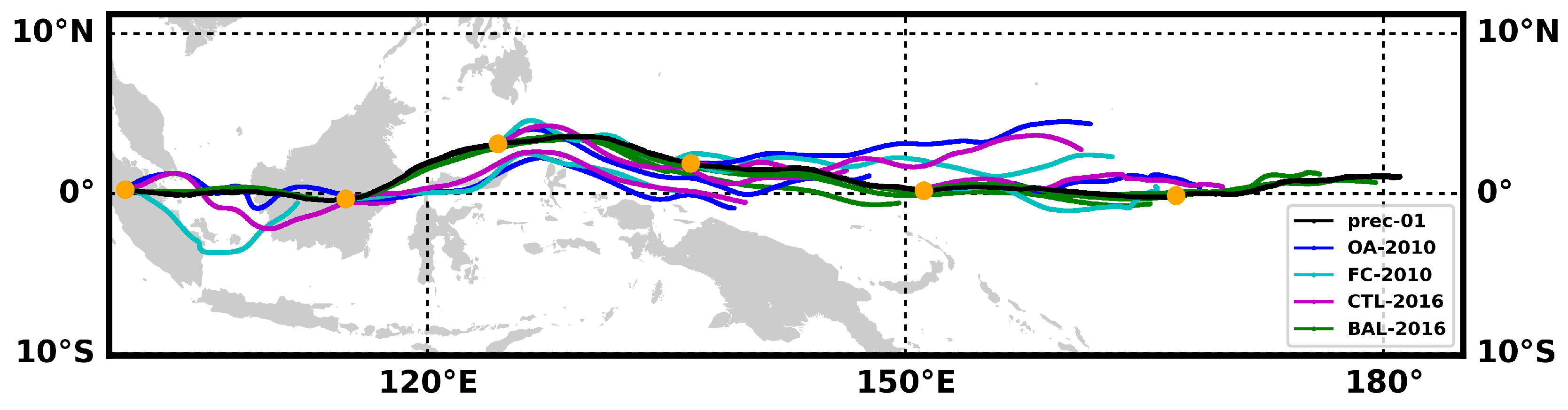
Figure 7 shows the real and calculated trajectories for the same dates as those of Figure 3. In Figure 7, the trajectories computed with model-level winds closely follows the real trajectory, whereas those computed with pressure-level winds strikingly deviate from it. Figure 8 illustrates why the degraded vertical resolution suffices to lose the relevant information contained in the BAL-2016 analyses. A strong shear of nearly 20 ms⁻¹km⁻¹ was found to be present at the balloon flight level in the assimilated run, associated with a eastward wind disturbance likely induced by a Kelvin wave packet. This disturbance was not present in the 2016 control run, and the vertical resolution of the pressure levels was obviously not sufficient to resolve the wind variability induced by the wave packet. Coincidentally, the BAL-2016 wind profile at the low vertical resolution was almost similar to that of CTL-2016 on model levels. This strongly suggests that a high vertical resolution is necessary to compute accuracte trajectories in the tropical UTLS. In practice, the operational forecasts during the Strateole-2 campaigns will be available on model levels, so this is not a concern for this specific application. More generally however, this result suggests that errors in trajectory calculations in the tropical UTLS are very sensitive to the vertical resolution, as this region is prone to large vertical shears associated either with equatorial waves or the QBO. The pre-Concordiasi period was obviously very special in this respect, since it corresponded to the QBO westerlies to easterlies reversal with Kelvin waves close to their critical levels. Air parcel trajectories computed with insufficient resolution may thus miss a significant part of this variability, and thus include large errors.

5. Pathways for Enhanced Accuracy

The accuracy to be expected for trajectory forecasts in the coming Strateole-2 campaigns lies in-between the results obtained for CTL-2016 (which incorporates a number of model upgrades) and those obtained for BAL-2016 (close to maximal accuracy because they use analyses and not forecasts). The range between the two extremes is large, and the low accuracy end of this range is rather poor. However, these are statistics obtained over the whole tropical band and for the entire 3-month flight. In operations, there will be ways to expect an enhanced accuracy, for temporally and/or spatially localised regions.

5.1. Regional Analysis of Trajectory Errors

Podglajen et al. [16] have emphasized that the largest errors in the tropical UTLS winds are found in specific regions such as over the Indian Ocean, and over the Eastern and Central Pacific (see their Figure 10), in agreement with Baker and co authors [5]. The geographical distribution of these errors in the modelled winds simply reflects the paucity of wind observations in these regions. To quantify how this zonal asymmetry in wind errors translates into trajectory accuracies, we have divided the tropics into four longitudinal sectors, and Figure 9 reports the corresponding trajectory statistics. The four sectors roughly correspond to the Western Pacific (100° E–180° E), Eastern Pacific (180° W–80° W), South America, Atlantic Ocean and Africa (80° W–20° E), and Indian Ocean (20° E–100° E). In the CTL-2016 setup, we indeed observe large differencies in trajectory accuracies among the longitudinal sectors. The largest 25th–75th interquartile spread in longitudinal difference between the real and simulated balloon positions is found as expected over the Eastern Pacific, while the largest median error over the Indian Ocean. The remaining two sectors, where most of the low-latitude radiosounding stations and ground-based instrumented sites are located, exhibit better statistics. On the other hand, the trajectory accuracy is found to be very homogenous over all four sectors in the BAL-2016 setup.

These results therefore suggest that the overall CTL-2016 statistics in trajectory accuracy are likely over-pessimistic, and that significantly better balloon trajectory forecasts can be achieved over continental areas and when balloon winds are assimilated.

5.2. Temporal Evolution of the Error

Podglajen et al. [16] have highlighted that the occurrence of large errors in the modelled winds arises in episodes, stemming either from the underestimation or even the mere absence of large-scale features of the flow, notably Kelvin waves or mixed Rossby–gravity waves. Such features have broad horizontal lengthscales and last for several days, hence the associated errors in winds and in trajectory forecasts also present a certain coherence in time. The fact that errors have a temporal coherence is illustrated in Figure 10. Many of the results described in previous sections are recalled in this figure: The success of the data assimilation is illustrated by the strikingly smaller errors for the trajectories calculated with BAL-2016 (bottom panel). The fact that major errors occur in episodes is conspicuous for balloon 1 (blue curves), but it also is relevant for balloon 2.

Such time coherence in the modelled wind errors can be used in practice in trajectory computations by estimating the error in the forecast trajectories from the error in the recent past. To show the information carried by the recent error, Figure 11 displays a scatterplot of the error in position after 24 h against the most recent error, i.e., the error in the trajectory started 24 h earlier. The correlation coefficient of the past and future errors is 0.78 in the CTL-2016 setup. Hence, the temporal coherence of trajectory errors is such that a majority of situations with large errors may be anticipated. Trajectories calculated from BAL-2016 yield much weaker errors, as documented earlier, and the correlation for the weaker errors is poor. However, this has little consequence for operational planning as the challenge is rather to anticipate large errors.

6. Summary and Conclusions

The primary objective of this study was to estimate the accuracy that can be expected in trajectory forecasts of the upcoming Strateole-2 long-duration balloon flights in the tropical UTLS. This accuracy is quantified through statistics on the distance between simulated and real balloon positions after 24 h of calculated trajectory. The balloon flights used are those of the 2010 polar Concordiasi and tropical Pre-Concordiasi campaigns, which provide a rare opportunity to compare real UTLS trajectories with calculated ones.

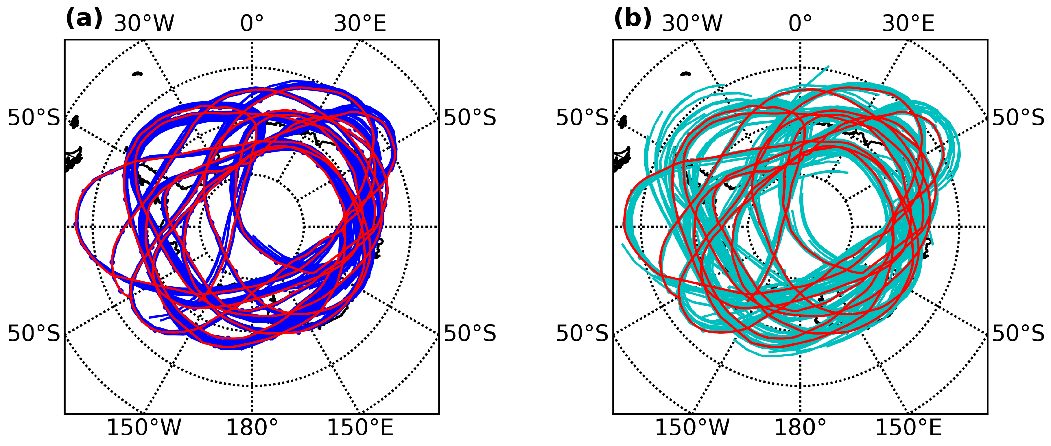
We have first compared the balloon trajectories with those computed with the 2010 ECMWF IFS operational model in order to understand the differences between analyzed and forecast winds. During the upcoming campaigns, the latter only will be relevant. In hindcast situations, the former provides an upper bound on the accuracy that may be hoped for.

At polar latitudes, the calculated trajectories behave as one expects: Both sets of trajectories are close to the real trajectories, and the error slightly increases when the forecast winds are used rather than the analysed winds. The median of the error in separation between the real and simulated balloons after 24 h is respectively 88 km and 108 km for the trajectories calculated with analyses, and forecasts, respectively. Note that the Concordiasi balloon winds were assimilated in the ECMWF IFS, making these estimates truly upper bound estimates for the accuracy.

In the tropics, results are in stark contrast with those at the pole: There are times when errors in model winds are so large that trajectories computed with either the analyses or forecasts bear little relation to the real trajectory. Separation errors are very anisotropic, and reflect a strong underestimation of westerly winds in the IFS model: After 24 h, the calculated trajectory has a 50% chance of being at a distance from the real balloon larger than ∼270 km when using the analyses, and ∼420 km when using the forecasts. For comparison, trajectories based on assuming persistence of the observed wind have a 50% chance of being at a distance larger than ∼370 km after 24 h. Such uncertainty is incompatible with an operational use of the forecast trajectories to plan coordinated observations between the balloons and groud-based instrumented sites. Yet, those statistics contitutes a pessimistic estimate of the expected trajectory accuracy during Strateole-2.

We then used winds issued by a more recent version of the ECMWF IFS model (CY43R1), with an increased vertical resolution. In the control setup in which balloon-borne winds were not assimilated, the accuracy of tropical balloon trajectories were found to be very similar to those computed in the 2010 model. This result emphasizes that the main factor limiting the model wind accuracy in the tropical UTLS is the paucity of wind observations in that region.

In contrast, tropical trajectories computed with analyses in the model setup that assimilated balloon-borne winds resulted in an accuracy comparable to that of the polar flights. Yet, this constitutes an upper bound for the accuracy of trajectories that will be computed during Strateole-2, since the favourable increments associated with the balloon wind observations may erode quickly in the forecasts. This might for instance be the case, if the balloon-borne increments are linked to a Kelvin wave packet, but are either too few to impose its large-scale structure in the model, or the model tends to damp these increments too rapidly.

We have nevertheless suggested that it is possible to estimate the accuracy of future balloon trajectories, knowing that of past trajectories. Several pieces of evidence [5,16] indeed suggest that modeled wind errors occur (i) primarily over the Indian and eastern Pacific oceans, which are regions where wind observations are sparse; and (ii) during episodes that last for several days. In operations, it will hence be possible to use the errors of the trajectories calulcated on a given day as an indication for the likely forecast errors for the next day.

Last, one should keep in mind that the Pre-Concordiasi balloons flew at levels close to the QBO wind reversal, making it possibly a particularly challenging period for wind forecasts. An attempt to compute trajectories with winds stored only on pressure levels actually stressed the importance of a high vertical resolution (i.e., a few hundred meters) to describe these strong vertical shears.

While this study focused on balloon trajectories, our conclusions likely have broader implications. Indeed, many investigations of UTLS processes use trajectory calculations, driven by analyses or reanalyses, even though it is difficult to estimate the accuracy of such calculations. The Pre-Concordiasi balloon flights provide a rare and unique opportunity to investigate errors in trajectory calculations in the tropical UTLS. The balloon trajectories are isopycnic, and hence they are less challenging than air parcel trajectories, which involve cross-isentropic displacements due to diabatic heating, in addition to the horizontal displacements. These diabatic heating rates constitute an additional source of uncertainty, so that errors found in balloon trajectories are likely lower estimates of the errors in air parcel trajectories. The fact that large errors are found after 24 h in our balloon trajectories emphasizes that air-parcel trajectory calculations in the tropical UTLS should be manipulated with caution. The largest errors are however localized in space and time, as they occured in episodes, over regions where wind observations are exremely sparse (Indian Ocean, eastern Pacific Ocean). This is not incompatible with previous case studies which convincingly showed, using complementary observations of water vapor in particular, trajectory calculations which provided insight on injection and transport of water vapor in the UTLS ([14,15], and B. Legras and S. Bucci, personal communication). Our results nonetheless emphasize the need for continued efforts to better understand processes and model error in the UTLS near the Equator, and to pay particular attention to uncertainties in trajectory calculations in process studies.

References

1. Fueglistaler, S.; Dessler, A.E.; Dunkerton, T.J.; Folkins, I.; Fu, Q.; Mote, P.W. Tropical Tropopause Layer. Rev. Geophys. 2009, 47. [Google Scholar] [CrossRef]
2. Folkins, I.; Martin, R. The vertical structure of tropical convection and its impacts on the budgets of water vapor and ozone. J. Atmos. Sci. 2005, 62, 1560–1573. [Google Scholar] [CrossRef]
3. Butchart, N. The Brewer-Dobson circulation. Rev. Geophys. 2014, 52, 157–184. [Google Scholar] [CrossRef]
4. Haiden, T.; Janousek, M.; Bauer, P.; Bidlot, J.; Dahoui, M.; Ferranti, L.; Prates, F.; Richardson, D.; Vitart, F. Evaluation of ECMWF forecasts, including 2014–2015 upgrades. ECMWF Tech. Memo 2015, 765, 51. [Google Scholar]
5. Baker, W.; Atlas, R.; Cardinali, C.; Clement, A.; Emmitt, G.D.; Gentry, B.M.; Hardesty, R.M.; Källén, E.; Kavaya, M.J.; Langland, R.; et al. Lidar-Measured Wind Profiles: The Missing Link in the Global Observing System. Bull. Am. Meteor. Soc. 2014, 95, 543–564. [Google Scholar] [CrossRef]
6. Solomon, S.; Rosenlof, K.; Portmann, R.; Daniel, J.; Davis, S.; Sanford, T.; Plattner, G.K. Contributions of Stratospheric Water Vapor to Decadal Changes in the Rate of Global Warming. Science 2010, 1219–1223. [Google Scholar] [CrossRef] [PubMed]
7. Riese, M.; Ploeger, F.; Rap, A.; Vogel, B.; Konopka, P.; Dameris, M.; Forster, P. Impact of uncertainties on atmospheric mixing on simulated UTLS composition and related radiative effects. J. Geophys. Res. Atmos. 2012, 117, 2156–2202. [Google Scholar] [CrossRef]
8. Holton, J.; Gettelman, A. Horizontal transport and the dehydration of the stratosphere. Geophys. Res. Lett. 2001, 28, 2799–2802. [Google Scholar] [CrossRef]
9. Liu, Y.; Fueglistaler, S.; Haynes, P. Advection-condensation paradigm for stratospheric water vapor. J. Geophys. Res. 2010, 115. [Google Scholar] [CrossRef]
10. Randel, W.; Jensen, E. Physical processes in the tropical tropopause layer and their roles in a changing climate. Nat. Geosci. 2013, 6, 169–176. [Google Scholar] [CrossRef]
11. Jensen, E.J.; Ueyama, R.; Pfister, L.; Bui, T.V.; Alexander, M.J.; Podglajen, A.; Hertzog, A.; Woods, S.; Lawson, R.P.; Kim, J.E.; et al. High-frequency gravity waves and homogeneous ice nucleation in tropical tropopause layer cirrus. Geophys. Res. Lett. 2016, 43, 6629–6635. [Google Scholar] [CrossRef]
12. Fujiwara, M.; Hasebe, F.; Shiotani, M.; Nishi, N.; Vömel, H.; Oltmans, S. Water vapor control at the tropopause by equatorial Kelvin waves observed over the Galapagos. J. Geophys. Res. 2001, 28, 3143–3146. [Google Scholar] [CrossRef]
13. Haag, W.; Kärcher, B.; Ström, J.; Minikin, A.; Lohmann, U.; Ovarlez, J.; Stohl, A. Freezing thresholds and cirrus cloud formation mechanisms inferred from in situ measurements of relative humidity. Atmos. Chem. Phys. 2003, 3, 1791–1806. [Google Scholar] [CrossRef]
14. Khaykin, S.; Pommereau, J.P.; Riviere, E.; Held, G.; Ploeger, F.; Ghysels, M.; Amarouche, N.; Vernier, J.; Wienhold, F.; Ionov, D. Evidence of horizontal and vertical transport of water in the Southern Hemisphere tropical tropopause layer (TTL) from high-resolution balloon observations. Atmos.Chem. Phys. 2016, 16, 12273–12286. [Google Scholar] [CrossRef]
15. Inai, Y.; Hasebe, F.; Fujiwara, M.; Shiotani, M.; Nishi, N.; Ogino, S.Y.; Vömel, H.; Iwasaki, S.; Shibata, T. Dehydration in the tropical tropopause layer estimated from the water vapor match. Atmos. Chem. Phys. 2013, 13, 8623–8642. [Google Scholar] [CrossRef]
16. Podglajen, A.; Hertzog, A.; Plougonven, R.; Žagar, N. Assessment of the accuracy of (re)analyses in the equatorial lower stratosphere. J. Geophys. Res. 2014, 119, 11166–11188. [Google Scholar] [CrossRef]
17. Hertzog, A.; Cocquerez, P.; Basdevant, C.; Boccara, G.; Bordereau, J.; Brioit, B.; Cardonne, A.; Guilbon, R.; Ravissot, A.; Schmitt, E.; et al. Stratéole/Vorcore—Long duration, superpressure balloons to study the Antarctic stratosphere during the 2005 winter. J. Ocean. Atmos. Technol. 2007, 24, 2048–2061. [Google Scholar] [CrossRef]
18. Rabier, F.; Bouchard, A.; Brun, E.; Doerenbecher, A.; Guedj, S.; Guidard, V.; Karbou, F.; Peuch, V.-H.; Amraoui, L.E.; Puech, D.; et al. The Concordiasi project in Antarctica. Bull. Am. Meteor. Soc. 2010, 91, 69–86. [Google Scholar] [CrossRef]
19. Fleming, R.J.; Kaneshige, T.M.; McGovern, W.E.; Bryan, T.E. The Global Weather Experiment II. The second Special Observing Period. BAMS 1979, 60, 1316–1322. [Google Scholar] [CrossRef]
20. Haase, J.; Alexander, M.; Hertzog, A.; Kalnajs, L.; Deshler, T.; Davis, S.; Plougonven, R.; Coquerez, P.; Venel, S. Around the world in 84 days. EOS 2018, 99. [Google Scholar] [CrossRef]
21. Podglajen, A.; Hertzog, A.; Plougonven, R.; Legras, B. Lagrangian temperature and vertical velocity fluctuations due to gravity waves in the lower stratosphere. Geophys. Res. Lett. 2016, 43, 3543–3553. [Google Scholar] [CrossRef]
22. Spichtinger, P.; Krämer, M. Tropical tropopause ice clouds: A dynamic approach to the mystery of low crystal numbers. Atmos. Chem. Phys. 2013, 13, 9801–9818. [Google Scholar] [CrossRef]
23. Dinh, T.; Legras, B.; Podglajen, A.; Hertzog, A.; Plougonven, R. Effect of temperature variations on homogeneous ice nucleation. Atmos. Chem. Phys. 2016, 16, 35–46. [Google Scholar] [CrossRef]
24. Podglajen, A.; Plougonven, R.; Hertzog, A.; Jensen, E. Impact of gravity waves on the motion and distribution of atmospheric ice particles. Atmos. Chem. Phys. 2018, 18, 10799–10823. [Google Scholar] [CrossRef]
25. Knudsen, B.M.; Christensen, T.; Hertzog, A.; Deme, A.; Vial, F.; Pommereau, J.P. Accuracy of analyzed temperatures, winds and trajectories in the Southern Hemisphere tropical and midlatitude stratosphere as compared to long-duration balloon flights. Atmos. Chem. Phys. 2006, 6, 5391–5397. [Google Scholar] [CrossRef]
26. Boccara, G.; Hertzog, A.; Basdevant, C.; Vial, F. Accuracy of NCEP/NCAR reanalyses and ECMWF analyses in the lower stratosphere over Antarctica in 2005. J. Geophys. Res. 2008, 113. [Google Scholar] [CrossRef]
27. Hoffmann, L.; Hertzog, A.; Rößler, T.; Stein, O.; Wu, X. Intercomparison of meteorological analyses and trajectories in the Antarctic lower stratosphere with Concordiasi superpressure balloon observations. Atmos. Chem. Phys. 2017, 17, 8045–8061. [Google Scholar] [CrossRef]
28. Stohl, A. Computation, accuracy and applications of trajectories—A review and bibliography. Atmos. Environ. 1998, 32, 947–966. [Google Scholar] [CrossRef]
29. Rabier, F.; Cohn, S.; Cocquerez, P.; Hertzog, A.; Avallone, L.; Deshler, T.; Haase, J.; Hock, T.; Doerenbecher, A.; Wang, J.; et al. The Concordiasi Field Experiment over Antarctica: First Results from Innovative Atmospheric Measurements. BAMS 2013, 94, ES17–ES20. [Google Scholar] [CrossRef]
30. Hertzog, A.; Basdevant, C.; Vial, F.; Mechoso, C.R. The accuracy of stratospheric analyses in the northern hemisphere inferred from long-duration balloon flights. Q. J. R. Meteorol. Soc. 2004, 130, 607–626. [Google Scholar] [CrossRef]
31. Anderson, J.; Hoar, T.; Reader, K.; Liu, H.; Collins, N.; Torn, R.; Avellano, A. The Data Assimilation Research Testbed: A community facility. Bull. Am. Meteorol. Soc. 2009, 90, 1283–1296. [Google Scholar] [CrossRef]
Figure 1. Trajectory of Concordiasi balloon 14, from 16 October to 22 December 2010 (red). Also plotted are trajectories calculated with (a) OA-2010 analyses (dark blue, left panel), and (b) FC-2010 forecasts (cyan, right panel). Simulated trajectories are started every 6 h from the real balloon positions, and last each for three days.
Atmosphere 10 00102 g001
Figure 2. Probability Density Function (PDF) of spherical distance between the real and simulated balloon trajectories during the Concordiasi campaign with the ECMWF 2010 operational analyses (blue), and forecasts (red).
Atmosphere 10 00102 g002
Figure 3. Pre-Concordiasi balloon 1 trajectory (black line) and those calculated with winds from OA-2010 (blue), FC-2010 (cyan), CTL-2016 (purple) and BAL-2016 (green). The period depicted starts on 31 March 2010, while the real balloon is drifting eastward toward South America. Calculated trajectories shown here start every day along the real balloon flight, and last three days. Filled orange circles are shown every 24 h on the real balloon trajectories.
Atmosphere 10 00102 g003
Figure 4. Same as Figure 3, but for the period starting on 19 March 2010.
Atmosphere 10 00102 g004
Figure 5. Probability Density Functions (PDF) of (a) longitudinal and (b) latitudinal error in the position of the simulated tropical balloons after 24 h, for trajectories calculated with winds from OA-2010 (dark blue), FC-2010 (light blue), and CTL-2016 (purple). Note that the horizontal axis covers 20°, i.e., about 2200 km, and that the PDFs in longitudes are asymmetric, in contrast to those in latitudes.
Atmosphere 10 00102 g005
Figure 6. Same as Figure 5 but for the IFS BAL-2016 setup, in which the balloon-measured winds have been assimilated. Note the difference in the horizontal-axis range when compared with Figure 5.
Atmosphere 10 00102 g006
Figure 7. Same as Figure 3, but for BAL-2016 trajectories computed either on model levels (dark green) or on pressure levels (light green). The vertical resolution of the archived winds is about 10 times higher on model levels than on pressure levels (250 m vs. 2.5 km).
Atmosphere 10 00102 g007
Figure 8. Vertical profiles of the zonal wind at the time and location corresponding to the first set of simulated trajectories shown in Figure 7: OA-2010 (blue) and BAL-2016 (dark green) on model levels, as well as BAL-2016 on pressure levels (light green). The black horizontal line indicates the balloon flight level.
Atmosphere 10 00102 g008
Figure 9. Summary of the balloon trajectory errors in longitudes (x-axis) and latitudes (y-axis) after 24 h of simulation for the different IFS setups. The left panel displays the errors statistics obtained over the whole tropics, while the right panel displays those errors in different longitude ranges for the CTL-2016 and BAL-2016 setup. Shown are the 25th–75th interquartile error spreads both in longitude and latitude. The two spreads cross at the median longitudinal and latitudinal errors. The latitude scale on the y-axis is represented by horizontal (either dotted or solid) lines that are plotted every degree. Dotted lines correspond to a 0° error in latitude for the IFS setup (right panel) or longitude range (left panel) indicated along the y-axis.
Atmosphere 10 00102 g009
Figure 10. Time series of spherical distance between the real and simulated balloon positions after 24 h of simulation, for the three PreConcordiasi balloons. The simulated trajectories are calculated using the OA-2010 (top panel), CTL-2016 (middle panel) and BAL-2016 (bottom panel) IFS setups.
Atmosphere 10 00102 g010
Figure 11. Scatterplot of the error in position after 24 h (vertical axis), as a function of the error in the trajectory started 24 h earlier (horizontal axis), for simulations using CTL-2016 (purple) and for those using BAL-2016 (green). Note the logarithmic axes. The linear correlation coefficients (R) and slope of the regression line (m) in log-log space are provided in the figure.
Atmosphere 10 00102 g011