Abstract
A low-frequency inertial atmospheric gravity wave (AGW) event was studied with lidar (40.5° N, 116° E), meteor radar (40.3° N, 116.2° E), and TIMED/SABER at Beijing on 30 May 2012. Lidar measurements showed that the atmospheric temperature structure was persistently perturbed by AGWs propagating upward from the stratosphere into the mesosphere (35–86 km). The dominant contribution was from the waves with vertical wavelengths and wave periods . Simultaneous observations from a meteor radar illustrated that MLT horizontal winds were perturbed by waves propagating upward with an azimuth angle of , and the vertical wavelength () and intrinsic period () of the dominant waves were inferred with the hodograph method. TIMED/SABER measurements illustrated that the vertical temperature profiles were also perturbed by waves with dominant vertical wavelength . Observations from three different instruments were compared, and it was found that signatures in the temperature perturbations and horizontal winds were induced by identical AGWs. According to these coordinated observation results, the horizontal wavelength and intrinsic phase speed were inferred to be ~560 km and ~21 m/s, respectively. Analyses of the Brunt-Väisälä frequency and potential energy illustrated that this persistent wave propagation had good static stability.
1. Introduction
It is widely recognized that atmospheric gravity wave (AGW) activity has a profound effect on general circulation patterns, temperature structure, and the spatial distributions of atmospheric gas mixing ratios by transporting energy and momentum from the troposphere into the middle and upper atmosphere [1]. Since Hines’ seminal work [2], many observational and theoretical research about the characteristics and effects of AGWs in the lower, middle, and upper atmosphere have been carried out at different locations in the world [3,4,5].
AGWs can be effectively studied with various ground-based remote sensing techniques, such as lidar, airglow imaging, and radar [6,7,8,9,10,11,12,13]. Lidar observation is an effective method to study medium and low-frequency AGWs from the troposphere up to the lower thermosphere, and it can be carried out quasi-permanently with high temporal and spatial resolutions. Airglow imaging can be used to directly study the two-dimensional horizontal characteristics of AGWs in the mesosphere and lower thermosphere (MLT) with high temporal and horizontal resolutions. Medium and large scale AGWs with periods of several hours can be measured with radar, and some intrinsic wave propagation parameters can be derived using winds observed with radar. Recently, satellite observations (e.g., TIMED/SABER, SOFIE/AIM) was used by researchers to analyze AGW activities in the middle and upper atmosphere, and it was proved that satellite observations are sensitive to low-frequency AGWs with horizontal and vertical wavelengths longer than ~100–200 km and ~4 km, respectively [14,15,16].
For a comprehensive study of AGW activities in the middle and upper atmosphere, coordinated observations from multiple instruments are likely more efficient, and it has become a tendency in the past decade. Although lidar observation is powerful for the study of AGW activities in the middle and upper atmosphere, only the vertical structure of AGWs can be probed with this method. Meteor radar has an advantage in measuring the background winds in the mesopause region, and it also cannot be used to directly explore the horizontal wave structures. Airglow imager can be used to observe the horizontal wave structures, but the vertical structure of AGWs cannot be directly measured with it. Meanwhile, because the horizontal wave-field of AGW is often inhomogeneous, it is generally difficult for those ground-based instruments to monitor the spatial variations of AGW activities. In this respect, satellite observations can be a valuable complement to conventional ground-based and in situ observations of AGWs. By using a temperature lidar and two meteor radars, gravity waves observed by airglow imagers were investigated by Nielsen et al. [17] during the MaCWAVE winter campaign. Similarly, after the background conditions of temperature and winds were respectively measured with lidar and meteor radar, AGWs that were simultaneously observed with airglow imagers were studied by Ejiri et al. [18]. By conducting a coordinated observation using airglow imager, sodium temperature lidar and radar, AGW dynamics observed by airglow were studied by Suzuki et al. [10,19] in Japan and Norway.
Although an enormous amount of observational studies regarding the characteristics and effects of AGWs in the middle and upper atmosphere have been published in the past several decades [5,9,20,21], most of them focused on the AGW activities observed in the MLT region, and few activities of larger scale AGWs propagating from the stratosphere into the mesosphere have been reported. By combining different types of lidar observations (i.e., sodium or potassium resonance lidar, Rayleigh lidar, Raman lidar, and Doppler lidar), several cases of AGW propagation from the stratosphere into the lower thermosphere have been reported by Rauthe et al. [22] in Germany (54° N, 12° E), Lu et al. [23] near Hawaii (19.5° N, 155.6° E), and Baumgarten et al. [24] in northern Norway (69° N, 16° E).
With support from the Chinese Meridian Project, coordinated observations and studies of AGW activities in the middle and upper atmosphere over China can be realized by conducting simultaneous observations from lidar, airglow imager, and radar at different observation stations. However, for AGW observations with coordinated instruments in China, only one case study of an MLT gravity wave has been reported so far [25]. In this paper, with the coordinated observations from lidar (40.5° N, 116° E), meteor radar (40.3° N, 116.2° E) and TIMED/SABER, a persistent and dominant AGW event observed in the middle and upper atmosphere over Beijing will be studied. This work attempts to give a comprehensive picture of this special mesoscale AGW propagation from the stratosphere into the mesosphere (35–86 km), regarding vertical and horizontal wavelengths, intrinsic period, phase speed, propagation directions, and static stability.
2. Instrumentation and Observation Results
The locations of the two ground-based observation stations and TIMED/SABER (the Sounding of the Atmosphere using Broadband Emission Radiometry aboard the satellite Thermosphere–Ionosphere–Mesosphere Energetics and Dynamics) footprints are depicted in Figure 1. The Yanqing (40.5° N, 116° E) lidar station was built in early 2010 [26]. Its lidar system works with two laser beams (532 nm and 589 nm), and their emitted energies are approximately 320 mJ and 60 mJ per shot, respectively. For an individual lidar profile, the photon counts accumulate for every 5000 laser shots in 3 min, and the spatial resolution and temporal resolution are 96 m and 3 min, respectively. The Shisanling (40.3° N, 116.2° E) meteor radar station was established in 2002. Atmospheric winds over an altitude range of 70–110 km can be measured by this radar with 2 km altitude and 1 h temporal resolution [27]. The TIMED satellite was launched into orbit with an altitude of 625 km and inclination of 74.1° in the December of 2001. The SABER instrument on board the TIMED satellite has measured temperature and several trace species profiles from ~20 km to ~110 km since January of 2002 [28]. It is using a limb-scanning measurement technology, and the average spatial resolution is ~0.4 km. The latitude coverage shifts from 53° N–83° S to 53° S–83° N, due to the yaw cycle of ~60 days. The SABER temperature retrieval procedure and validation have been reported by Remsberg et al. [29], and the system errors in temperature profiles are 1–2 K under the altitude of 100 km.
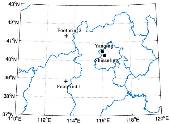
Figure 1.
Map showing the station locations and the footprints of TIMED/SABER. The observation stations marked with black dots are Yanqing (40.5° N, 116° E) and Shisanling (40.3° N, 116.2° E). Satellite footprints marked with crosses are footprint 1 (38.87° N, 113.49° E) and footprint 2 (41.27° N, 113.44° E).
2.1. Lidar-Observed Atmospheric Temperature Structure and Wave Propagation
By employing the method introduced in the references [6,30,31], atmospheric temperature in the 35–87 km altitude range was retrieved from the photon counts of the Rayleigh backscatter assuming hydrostatic equilibrium, and the altitude-time contour of temperature was plotted in Figure 2 according to the dual-wavelength lidar observations at nighttime on 30 May 2012.
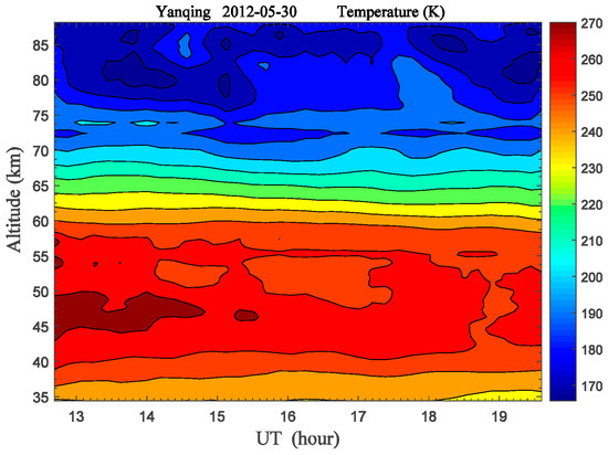
Figure 2.
Atmospheric temperature structure (35–87 km) derived from the dual-wavelength Rayleigh lidar observations at Yanqing (40.5° N, 116° E) at nighttime on 30 May 2012.
Here, the back-scattered signal at 532 nm is used as a high-sensitivity channel to measure the atmospheric temperature at an altitude range of 56–87 km, and the signal at 589 nm is used as a low-sensitivity channel to measure the atmospheric temperature at 35–56 km altitude. When deriving the atmospheric temperature profile, in order to increase the signal-to-noise ratio (SNR) and extend the upper altitude limit of integration, photon profiles were spatially and temporally added simultaneously to obtain profiles with a 384 m spatial resolution and a 25 min temporal resolution. The relative error of lidar-measured temperature is inversely proportional to the RMS photon counts [32]. The temperature uncertainty is set to <5% at different altitudes, and the upper altitude limit reached 87 km after data calibration [31,33]. Temperature values from the NRLMSISE-00 model data are used for each temperature profile derivation at an altitude of 89 km.
Temperature deviations from the nightly mean were calculated at different altitudes, and the relative temperature perturbation, (=), was plotted in Figure 3a. Coherent wave structures shown by the dotted lines in the figure indicate that the temperature structure (35–86 km) was obviously perturbed by multiple AGWs during lidar observation. The downward phase progress indicates that the wave energy was transported upward [34]. To reveal the contribution from AGWs with different vertical wavelengths, the vertical wavenumber power spectra, , was calculated for each temperature perturbation profile by a Fourier transform using the autocorrelation function. The analysis results are plotted versus the observation time in Figure 3b.
where is the autocorrelation function of the relative temperature perturbation in a spatial sequence, and s represents the predetermined altitude difference for sampling.
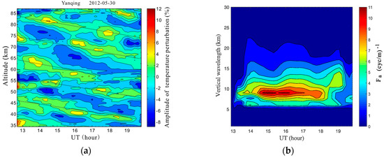
Figure 3.
(a) Lidar-observed relative temperature perturbation at nighttime on 30 May 2012. The black dotted lines were plotted manually to show the coherent temperature perturbation structures. (b) Corresponding vertical wavenumber power spectra for the temperature perturbations associated with gravity waves.
The black dotted lines in Figure 3a illustrate that the wave perturbations had similar structures throughout the observed altitudes and persisted for the entire lidar observation time. On the other hand, Figure 3b shows that the time-varying power spectra were obviously dominant and the contribution mainly came from AGWs with vertical wavelengths of ~8–10 km. These results may suggest that the persistent waves observed at different altitudes possibly originated from the same wave packet and represented the same dominant wave mode. Thus, an average vertical phase velocity, , was first estimated from the mean slope of the dotted lines in Figure 3. Then, the observed wave period, , was calculated with .
Of course, since a nightly mean method is employed to obtain the temperature perturbations, the influences from tides have not been effectively eliminated [35,36]. However, vertical wavelengths of the diurnal tide are generally greater than 20 km in the middle and upper atmosphere at the mid-latitudes [27,37,38]. The semidiurnal tide and terdiurnal tide have even longer wavelengthes, as well. Therefore, it was believed that those wave-like temperature perturbation structures, shown in Figure 3 were associated with AGW activity.
2.2. Background Wind and Wave Propagation Observed by Meteor Radar
To our knowledge, due to the rapid decrease of atmospheric density, AGWs usually have large amplitude near the mesopause region. After the contributions from the mean background flow, planetary waves and tides are removed, many observations report that wind profiles measured by meteor radar are often obviously perturbed by AGWs with vertical scales ranging from 5 km to 15 km [13,39,40]. Here, the MLT horizontal winds were simultaneously measured with meteor radar at Shisanling (40.3° N, 116.2° E), and the observation data were analyzed with the method introduced by Tsuda et al. [39]. The mean background wind in the altitude range of 76–106 km is plotted in the left panel of Figure 4, and the corresponding wind perturbations are plotted in the right panel. Noted that both the northward and the eastward winds had positive values in the figures. The wind perturbations were obtained by applying a bandpass filter, with cutoffs at 5 km and 17 km, after the mean background flow was removed from the observation data [13,39].
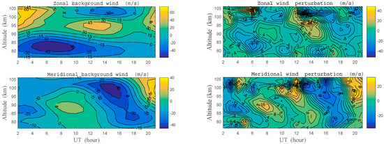
Figure 4.
The mean background horizontal wind (left panel) and wind perturbations (right panel) measured simultaneously with meteor radar at Shisanling (40.3° N, 116.2° E) on 30 May 2012. Positive values in the figures indicate the northward meridional wind or the eastward zonal wind.
In Figure 4, both the zonal wind and the meridional wind perturbations present fair wave-like structures. This result means that wave propagation in the MLT region was simultaneously observed by meteor radar at Shisanling. To extract more details of these wave propagations, meteor radar observations at 16 UT were analyzed, and the corresponding hodograph is plotted in Figure 5. The hodograph of wind perturbations in the altitude range of 76–86 km was fitted with an ellipse in Figure 5b using the least squares method [24,39,41]. The fitting results show that the wind vector rotated clockwise as altitude increased, indicating upward energy transportation with a downward phase velocity. The horizontal direction of wave propagation was along the major axis of the ellipse, but it had a 180° ambiguity unless the relationship was clear between the perturbations of wind and temperature [9,24,41]. On the basis of temperature measurement from lidar (i.e., Figure 3a), the hodograph was analyzed in Figure 5c for the perturbations of zonal wind and temperature in the 76–86 km altitude range. It is found that the vector rotated anticlockwise in Figure 5c with increasing altitude. Since the two vectors rotate contrarily in Figure 5 with increasing altitude, it is determined that those waves propagated toward the southwest with an azimuth , as shown by the black arrow in Figure 5b. Here, the azimuth means the angle between the major axis of the ellipse and normal North direction.
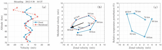
Figure 5.
(a) Vertical profiles of horizontal wind perturbations measured with meteor radar at 16 UT on 30 May 2012. A bandpass filter was applied to the wind data, with cutoffs at 5 km and 17 km. (b) Hodograph analysis for zonal and meridional wind perturbations. By using the least squares method, hodograph (solid line with dots) was fitted with an ellipse (red dashed line) in the 76–86 km altitude range. The black arrow indicates the horizontal wave propagation direction. (c) Hodograph analysis for zonal wind and temperature perturbations in the 76–86 km altitude range.
Moreover, the two extremities of the semimajor axis are located at approximately 80 km and 85 km in Figure 5b, indicating that a dominant vertical wavelength of ~ was measured for AGWs in this altitude range. The amplitudes of the semimajor and semiminor axes of the ellipse are 14.7 m/s and 5.9 m/s, respectively, with a ratio of 2.5. According to the linear polarization relation for inertial AGWs, the intrinsic frequency can be calculated with Equation (2), and an intrinsic period was inferred for the dominant waves [39]
where and represent the horizontal perturbation velocities parallel and perpendicular to the azimuth of the propagation vector, respectively. Variable f represents the inertial frequency, and the corresponding inertial period at the latitude of Shisanling is .
2.3. Wave Structures Observed by TIMED/SABER
The temperature data measured by TIMED/SABER near Beijing (i.e., at footprint 1 and footprint 2 in the map) on 30 May 2012 were analyzed, and the AGW parameters were extracted with a method similar to that described by Fetzer and Gille [42], Preusse et al. [14,43], Yamashita et al. [44], and Liu et al. [16,45]. The temperature structure (30–87 km) measured at ascending nodes near 40.5° N was plotted in Figure 6a. Here, the temperature profiles () in the latitude band of 38–43° N are rearranged in the order of increasing longitude to produce a longitude-altitude temperature distribution. To minimize the influence of tides on GWs, this rearrangement was only performed on the data measured at ascending nodes, and the mean latitude was 40.22° N with a standard deviation of 1.31° [43,44,45,46]. The background temperature () was obtained and plotted in Figure 6b by applying a least square harmonic fitting to the temperature structure at each altitude. The corresponding zonal wavenumbers were set to , such that tides and planetary waves can be eliminated efficiently, since they have longer horizontal wavelengths [43,44,46]. By removing the background temperature from the observed temperature, the residuals (Figure 6c) were regarded as the temperature perturbations () induced by AGWs. With this harmonic analysis method, TIMED/SABER observations are sensitive to low-frequency AGWs with horizontal and vertical wavelengths longer than ~100–200 km and ~4 km, respectively [14,15].
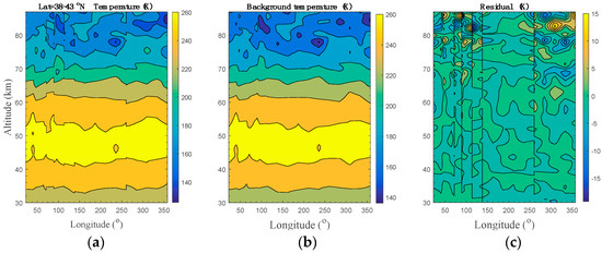
Figure 6.
TIMED/SABER measurement results on 30 May 2012. (a) Temperature structure observed in the latitude range of 38–43° N. (b) Background temperature obtained by the least square harmonic fitting with zonal wavenumbers from 0 to 7. (c) Residual (temperature perturbation) obtained by subtracting the fitted background temperature from the observed temperature.
To focus on the measurements at the two footprints near Beijing in the map, the relative temperature perturbation profiles () were calculated with first; and then, wavelet analysis (i.e., morlet) was performed to obtain the main wave components [47]. Finally, a new temperature perturbation profile was reconstructed with the three dominant wave components. These results are plotted in Figure 7a,b, and at both footprints, in the altitude range of 30–86 km, the temperature profiles were perturbed by AGWs with vertical wavelengths of approximately 6–10 km. Furthermore, a phase comparison was made for the wave propagations at different altitudes in Figure 7c. It is interesting to find that the phase varied entirely contrarily with the increasing altitude at the two footprints. Since the time lag was less than 1 min, the temperature profiles at the two footprints were measured by TIMED/SABER approximately at the same time. This suggests that the horizontal distance between the two footprints in Figure 1 is approximately the odd times of the half wavelength.
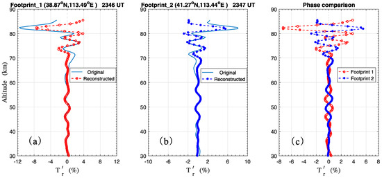
Figure 7.
Wave structures observed by TIMED/SABER at footprint 1 (38.87° N, 113.49° E) and footprint 2 (41.27° N, 113.44° E) on 30 May 2012. (a) The relative temperature perturbation (solid line) observed at footprint 1 and the reconstructed AGW profile (dashed line with circles) by wavelet filter. (b) The relative temperature perturbation (solid line) observed at footprint 2 and the reconstructed AGW profile (dashed line with dots) by wavelet analysis. (c) Phase comparison between AGW propagations observed at the two footprints.
3. Comparisons and Discussion
3.1. Temperature Measurement Comparison
In Figure 8a, the lidar-measured temperature profile was compared to the simultaneous measurement from TIMED/SABER at 1433 UT. The corresponding result from the NRLMSISE-00 empirical model (http://ccmc.gsfc.nasa.gov/modelweb/models_home.html) was also plotted for comparison with a red dashed line. The spatial resolution of the SABER/TIMED measurement is 0.5 km, and it is 0.2 km for the results from the NRLMSISE-00 model.
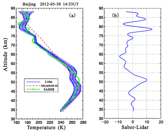
Figure 8.
Temperature measurement comparison. (a) Temperature profiles measured by lidar and TIMED/SABER over Beijing at 1433 UT on 30 May 2012. The red dashed line indicates the temperature profile from the NRLMSISE-00 model. The horizontal bars represent standard deviations of the lidar-measured temperature. (b) Temperature difference (SABER-lidar) between the lidar and TIMED/SABER measurements at different altitudes.
In Figure 8a, the comparisons show that in the altitude region of 35–87 km, similar variation tendencies in the temperature profile were shown by the three methods. Moreover, in Figure 8b, the maximum temperature difference between the measurement results from lidar and SABER was less than 15 K. That is, temperature structures (plotted in Figure 2) measured by the dual-wavelength lidar over Beijing were reliable. Meanwhile, the measurement differences at different altitudes in Figure 8b were likely related to the following two facts:
- The atmospheric temperature profile was measured by lidar at Yanqing (40.5° N, 116° E) using a vertical detection method, and the temperature profile was measured by SABER using the limb-scanning measurement technique when the TIMED satellite was over Beijing (40.406° N, 105.605° E) at 1433 UT; and
- There are some temporal differences between the two measurements. To improve the accuracy, the sampling period was set to 25 min for the lidar measurement, but it was 36 s for the TIMED/SABER measurement.
3.2. Phase Relations between the Temperature and Wind Perturbations
Because the horizontal distance between Yanqing (40.5° N, 116° E) and Shisanling (40.3° N, 116.2° E) is less than 40 km on the map, the same wave propagations could be simultaneously observed by lidar and meteor radar. Therefore, the phase relation between the lidar-observed temperature perturbation () and the wind perturbation () was analyzed in Figure 9. Note that, this means the perturbation of the k-ward horizontal wind calculated according to the meteor radar measurement results in Figure 4. The AGW linear theory gives the following relation (Equation (3)) between the perturbation of horizontal wind and temperature, i.e., temperature perturbation usually lags the k-ward horizontal wind by in phase [10,24].
where are the perturbations of the k-ward horizontal wind, are the temperature perturbations, is vertical wavelength, is horizontal wavelength, is the intrinsic frequency, i is the imaginary unit, g is gravity acceleration, and N is the Brunt-Väisälä frequency.
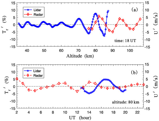
Figure 9.
Phase relations between the perturbations of temperature and horizontal wind. (a) Perturbation profiles of temperature (circle) and the k-ward horizontal wind (diamond) measured by lidar and meteor radar at 18 UT, respectively. (b) Time-varying perturbations of temperature (circle) and the k-ward horizontal wind (diamond) at an altitude of 80 km.
It is found in Figure 9a that at overlapping measurement altitudes (76–86 km), there is an average wave path-difference of ~2.4 km between the two curves. Meanwhile, it is shown by the simultaneous measurement results from lidar (Figure 3) and meteor radar (Figure 5) that the dominant vertical wavelength was approximately 10 km in this altitude range. Therefore, this average wave path-difference is approximately a quarter of the wavelength. That is, there was a phase-difference of approximately between the perturbations of temperature and horizontal wind at 18 UT.
In Figure 9b, the average time lag between the two curves is ~2.2 h. The dominant wave period was inferred to be in Figure 5. This average time lag is ~18% greater than the value of a quarter of the wave period. Thus, for the simultaneous measurements from lidar and meteor radar at an altitude of 80 km, there roughly existed a phase-difference of about between the perturbations of temperature and horizontal wind.
Indeed, the phase comparisons above are likely not so precise. It is probably because of the following two reasons:
- The spatial and temporal resolution of meteor radar measurements are 2 km and 1 h, respectively. Too much uncertainty probably exists in the wind data;
- The horizontal distance is ~40 km between the two observing locations, and there were some objective phase differences in the observed wave propagations.
However, the phase relations obtained above from realistic measurements were still roughly consistent with the prediction of the linear gravity wave theory. This may suggest that identical wave propagations were simultaneously observed by lidar at Yanqing (40.5° N, 116° E) and meteor radar at Shisanling (40.3° N, 116.2° E).
3.3. Atmospheric Gravity Wave Properties
For comparison, observation results of the dominant gravity waves from lidar, meteor radar, and TIMED/SABER are listed in Table 1, regarding the wavelengths, wave periods, and wave propagation direction.

Table 1.
Characteristics of the dominant gravity waves observed by lidar, meteor radar, and TIMED/SABER.
3.3.1. Wavelengths
In Table 1, lidar measurements show that the dominant vertical wavelength was 8–10 km in the altitude range of 35–86 km, meteor radar measurements illustrate the dominant vertical wavelength was ~10 km at the 76–86 km altitude range, and TIMED/SABER observations give a similar result with the dominant vertical wavelength of 6–10 km in the altitude range of 30–86 km. Although it is generally difficult to obtain an accurate one-to-one correspondence for specific AGW parameter values, due to the differences in their observation resolution, similar dominant vertical wavelengths were still observed at different altitudes with the three instruments.
To focus on the measurement results in the 76–86 km altitude range, a dominant vertical wavelength of ~10 km was derived in Figure 5 according to the meteor radar measurements at 16 UT. Both the lidar observation results in Figure 3 and the TIMED/SABER measurement results in Figure 7, illustrate a dominant vertical wavelength ~10 km in this altitude range. For the corresponding dominant horizontal wavelength of this dominant AGW at this altitude range, it can be estimated with the gravity wave linear dispersion relation [1].
where is the horizontal wavenumber vector, and is the k-ward horizontal wind velocity. c represents the ground-based horizontal phase speed, and is the scale height. denotes the Brunt-Väisälä frequency, and it can be calculated with Equation (5)
Here, at the 76–86 km altitude range, is estimated to be 20 m/s according to the meteor radar measurement results (Figure 4) around 16 UT. The term denotes the local temperature gradient, obtained according to the lidar measurements (Figure 2). cp represents the specific heat at constant pressure. By substituting into these simultaneous measurement results of temperature and wind from lidar and meteor radar, a corresponding horizontal wavelength was calculated with Equations (4–5). To combine the TIMED/SABER measurement result (Figure 7) that the horizontal distance between the two footprints in Figure 1 was approximately the odd times of the half wavelength, the value of the dominant horizontal wavelength was modified to ~560 km, since the horizontal distance between the two footprints is ~280 km in the map.
That is, the dominant vertical wavelengths of this AGW were observed to be 6–10 km at different altitude ranges by lidar, meteor radar, and TIMED/SABER. At an altitude range of 76–86 km, a dominant ~10 km vertical wavelength was observed by all of the three instruments. Since temperature and wind measurements were available, the dominant horizontal wavelength of this wave propagation was estimated at ~560 km with the linear dispersion relation.
3.3.2. Wave Periods and Propagation Direction
In Table 1, the lidar-observed wave period was 6.6 ± 0.7 h in the 35–86 km altitude range, and the hodograph analysis of meteor radar measurements (Figure 5) show that the intrinsic wave period was 7.4 h in the 76–86 km altitude range. That is, a low-frequency inertial AGW event was observed over Beijing. In general, due to the influence of background wind, wave periods observed by ground-based instruments are actually Doppler-shifted, and the relation between the observed period () and the intrinsic period () is
To confirm the reliability of the simultaneous measurement results of wave periods from lidar and meteor radar, the following values were substituted into Equation (6) to estimate the values of horizontal phase speed c and the ,
Here, it should be noted that the horizontal wavelength ~560 km and the intrinsic period 7.4 h were derived above from the coordinated measurements of meteor radar and TIMED/SABER in the 76–86 km altitude range. The observed 6 h wave period was from the measurement results around the altitude of 80 km (i.e., Figure 9b). The calculation results are and . This gives if the background wind is in the same direction as the propagated wave and if they are opposite. It is found from Figure 4 that, in the altitude range of 76–86 km, both the background zonal wind and the meridional wind seldom approach 50 m/s, and they are negative and less than 10 m/s during the most observations. Therefore, the first solution of is more probable, and the waves are propagating in a similar direction to background flow. Namely, the dominant wave is propagating toward the southwest with a 26 m/s horizontal phase speed, and the intrinsic horizontal phase speed is ~21 m/s. These analysis results are consistent with hodograph analysis results in Figure 5.
Regarding the wave propagation directions, lidar observations show that the waves propagate upward with a mean downward phase speed of ~0.38 m/s. The same result for the vertical propagation direction was confirmed by simultaneous observations from a meteor radar. For the horizontal wave propagation direction, meteor radar observations show that the waves were propagating toward southwest with an azimuth angle of 247°. Therefore, it is clear that, on that night, AGWs propagated obliquely upward from the stratosphere into the lower thermosphere at an azimuth angle of ~247°.
3.3.3. Static Stability
It is known that the real propagation process in the middle and upper atmosphere is complicated, and AGWs always dissipate, become saturated, or become broken, due to the influence of the mean background [1]. In this way, the transportation of energy and momentum is realized between the lower and upper atmosphere. However, in Figure 1, persistent wave propagation was observed for the entire nighttime, and the coherent wave-structure was only fairly disrupted at 55 km approximately 18 UT. For this reason, the Brunt-Väisälä frequency and AGW potential energy were calculated and analyzed according to the lidar measurements. Here, is calculated with Equation (5), and the potential energy of per unit volume is calculated as
where the atmospheric density profile is from the lidar measurements. By employing the method introduced by Guan at al. [33], photomultiplier tubes’ (PMT) pulse pile-up and signal-induced noise (SIN) calibrations have been made for lidar signals, and the uncertainty in the retrieved atmospheric density is less than 5% at different altitudes.
The time-altitude variation of is plotted in Figure 10a, and it is found that the background atmosphere under 80 km was stable for the entire night, and some unstable regions (i.e., ) only occurred near the mesopause. The nightly mean is plotted in Figure 10b, and it shows that the value was greater than at most altitudes. This means the background atmosphere had good convective stability for nighttime wave propagation on 30 May 2012. Moreover, the curve plotted in Figure 10c illustrates that AGW potential energy deceased gradually with increasing altitude under 80 km. This also means that no obvious wave breaking happened during the obliquely upward propagation from the stratosphere to the mesosphere. In addition, in Figure 10c, it is noticed that the nightly mean potential energy decreased by about two orders in the altitude range of 54–73 km. This means that the waves have dissipated at those altitudes, due to the influences of the mean background atmosphere. To compare with observation results of plotted in Figure 10a, it is found that they were marginally stable regions (i.e., ), and the waves were probably to saturate and dissipate in this persistent low-stability layer.
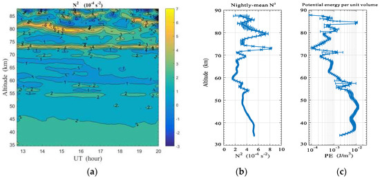
Figure 10.
(a) Time-altitude variation of the Brunt-Väisälä frequency N2, (b) nightly mean N2 profile, and (c) nightly mean profile of AGW potential energy per unit volume. The horizontal bars represent standard deviations.
Similar persistent gravity wave propagation event from the stratosphere to the mesosphere has been reported by Rauthe et al. [22] (their Figures 2 and 5) according to observations from the Rayleigh-Mie-Raman lidars in Germany (54° N, 12° E), and their wavelet spectrum analyses also revealed that the wave propagation was dominated by multiple AGWs with vertical wavelengths of 11–18 km in the middle and upper atmosphere. Additionally, their seasonal distribution analysis [16] (their Figure 8) shows that AGWs with the dominant vertical wavelength 6–20 km were more frequent. Another similar case was observed by Lu et al. [23] (their Figure 4) with lidars near Hawaii (19.5° N, 155.6° E). They reported that in the altitude range of 35–103 km (with a data gap at 76–84 km), the wave propagation was also dominated by AGWs with 6–13 km vertical wavelength, ~2140 km horizontal wavelength, and an ~15 h intrinsic period. Baumgarten et al. [24] (their Figure 3) also observed a persistent inertial gravity wave event in the middle atmosphere (20–80 km) with Doppler Rayleigh lidar in northern Norway (69° N, 16° E). They reported that the wavefield was also characterized by the presence of multiscale waves. In the 59.6–67 km altitude range, the dominant vertical wavelength was 5–10 km, and the mean intrinsic period was ~9.4 h.
To compare, the observation results of this persistent AGW event over Beijing are compatible with the lidar observations at Hawaii, Germany, and Norway. However, a significant difference is that, the wave propagation from the stratosphere into the mesosphere reported in this paper was coordinately studied with multiple instruments (i.e., lidar, meteor radar, and TIMED/SABER) at different locations. Measurements with multiple instruments at different locations are relatively more effective in the interpretation of the observed wave characteristics (e.g., modification to the horizontal wavelength estimation with TIMED/SABER measurements in this paper). On the other hand, A significant “damping layer” was observed around the stratopause region by Lu et al. [23] at Hawaii (19.5° N, 155.6° E), and their lidar observations showed that the wave experienced strong dissipation as it propagated through the damping layer. Some ‘‘nodes’’ in the temperature deviation profiles were also found at different altitudes by Rauthe et al. [22] in Germany (54° N, 12° E), and the wave amplitudes strongly decreased at those altitudes. For this case observed over Beijing, although no obvious wave breaking was observed, it was found that the waves gradually dissipated in the persistent low-stability layer (54–73 km). Therefore, the realistic propagation processes of AGWs from the lower atmosphere to the upper Atmosphere are often complicated, and the waves always get dissipated, saturated, or broken, due to the influences of the background atmosphere.
As far as we know, such kind of low-frequency inertial AGW propagating from the stratosphere to the mesosphere and persisting the entire night has not been reported in China. For the recent work from Jia et al. [25], it is an MLT gravity wave event observed mainly with airglow imager. Indeed, airglow imager observation is helpful to the direct measurements of the horizontal wave structure in the MLT region. Unfortunately, for the AGW event reported by us in this paper, we failed to identify waves with medium or large scales from the simultaneous observations of the OH airglow imager at Xinglong (40.2° N, 117.4° E). We ascribe the failure to the longer wave period (~7.4 h) comparative to the effective observation time of the airglow imager in that night. However, in our work, the atmospheric temperature perturbation in a larger vertical altitude range (35–86 km) was measured by the dual-wavelength lidar, and it is likely more relevant to observe AGWs at medium or large scales and helpful to present the details of the wave propagation process from the stratosphere into the upper mesosphere. Meanwhile, TIMED/SABER observations are a valuable complement to the measurement results from lidar and meteor radar, and useful information on the dominant vertical and horizontal wavelengths of AGW were provided by them.
4. Conclusions
By using lidar (40.5° N, 116° E), meteor radar (40.3° N,116.2° E), and TIMED/SABER, a low-frequency inertial AGW propagating obliquely from the stratosphere into the upper mesosphere and persisted for an entire night was observed over Beijing on 30 May 2012. At an altitude range of 35–86 km, temperature measurements from lidar show that AGWs propagated upward with a mean phase speed of ~0.38 m/s, and the dominant waves had a vertical wavelength and wave period . MLT winds were simultaneously measured by meteor radar, and hodograph analysis of wind perturbation shows that the waves propagated upward at an azimuth of . In the 76–86 km altitude range, the dominant vertical wavelength was ~10 km, and the intrinsic period was deduced to be 7.4 h. Gravity wave propagation was also observed by TIMED/SABER, and it was found that the dominant vertical wavelength was 6–10 km in the altitude range of 30–86 km. According to the coordinated measurements of temperature and horizontal winds, the dominant horizontal wavelength was calculated with the linear dispersion relation. The horizontal intrinsic phase speed was inferred to be ~21 m/s. Variations of the Brunt-Väisälä frequency and potential energy were analyzed, and it was found that these waves had good stability during their obliquely upward propagation.
It is the first time to comprehensively study such kind of persistent and dominant AGW event over China with coordinated instruments at different locations. Although it is generally hard to obtain an accurate one-to-one correspondence of measurement results from different instruments, comparisons between the measurements from lidar, meteor radar and TIMED/SABER proved that the signatures in the temperature perturbations and horizontal winds were induced by identical gravity wave propagations. For this type of low-frequency inertial AGW event propagating from the stratosphere into the mesosphere, it probably had relatively stable and strong sources in the lower atmosphere. Saturation, dissipation and breaking from such mesoscale waves should have a significant impact on the general circulation [21]. Therefore, this work could be helpful for the clarification of AGW contributions to atmospheric dynamics in the middle and upper atmosphere, and it is worth carrying out a long-term and deeper investigation on the wave generation, saturation and dissipation mechanisms with coordinated instruments in China.
Author Contributions
Formal analysis, S.G. and G.Y.; Investigation, S.G., X.L. and Q.L.; Resources, G.Y.; Writing—original draft preparation, S.G. Supervision, J.X.
Funding
This research was funded by the National Natural Science Foundation of China (grant numbers 41864005 and 41264006), and Project Supported by the Specialized Research Fund for State Key Laboratories.
Acknowledgments
The lidar observation data were obtained freely from http://www.meridianproject.ac.cn/, the meteor radar measurement data were downloaded freely from http://space.iggcas.ac.cn, and the TIMED/SABER measurement data were downloaded freely from http://saber.gats-inc.com/data.php. The authors are thankful to the TIMED/SABER team for the freely downloadable data, and we acknowledge the use of data from the Chinese Meridian Project and the Space Electromagnetic Environment Laboratory.
Conflicts of Interest
The authors declare no conflict of interest.
References
- Fritts, D.C.; Alexander, M.J. Gravity wave dynamics and effects in the middle atmosphere. Rev. Geophys. 2003, 41, 1003. [Google Scholar] [CrossRef]
- Hines, C.O. Internal atmospheric gravity waves at ionospheric heights. Can. J. Phys. 1960, 38, 1441–1481. [Google Scholar] [CrossRef]
- Hines, C.O. The saturation of gravity waves in the middle atmosphere, II. Development of Doppler–spread theory. J. Atmos. Sci. 1991, 48, 136Cl379. [Google Scholar] [CrossRef]
- Gardner, C.S. Diffusive filtering theory of gravity wave spectra in the atmosphere. J. Geophys. Res. 1994, 99, 20601–20622. [Google Scholar] [CrossRef]
- Yang, G.; Clemesha, B.; Batista, P.; Simonich, D. Gravity wave parameters and their seasonal variations derived from Na lidar observations at 23oS. J. Geophys. Res. 2006, 111, D21107. [Google Scholar] [CrossRef]
- Chanin, M.L.; Hauchecorne, A. Lidar observation of gravity and tidal waves in the stratosphere and mesosphere. J. Geophys. Res. 1981, 86, 9715–9721. [Google Scholar] [CrossRef]
- Sivakumar, V.; Rao, P.B.; Bencherif, H. Lidar observations of middle atmospheric gravity wave activity over a low-latitude site (Gadanki, 13.5° N, 79.2° E). Ann. Geophys. 2006, 24, 823–834. [Google Scholar] [CrossRef]
- Li, T.; She, C.-Y.; Liu, H.-L.; Leblanc, T.; McDermid, I.S. Sodium lidar-observed strong inertia-gravity wave activities in the mesopause region over Fort Collins, Colorado (41° N, 105° W). J. Geophys. Res. 2007, 112, D22104. [Google Scholar] [CrossRef]
- Gong, S.; Yang, G.; Dou, X.; Xu, J.; Chen, C.; Gong, S. Statistical study of atmospheric gravity waves in the mesopause region observed by a lidar chain in eastern China. J. Geophys. Res. Atmos. 2015, 120, 7619–7634. [Google Scholar] [CrossRef]
- Suzuki, S.; Nakamura, T.; Ejiri, M.K.; Tsutsumi, M.; Shiokawa, K.; Kawahara, T.D. Simultaneous airglow, lidar, and radar measurements of mesospheric gravity waves over Japan. J. Geophys. Res. 2010, 115, D24113. [Google Scholar] [CrossRef]
- Li, Q.; Xu, J.; Yue, J.; Yuan, W.; Liu, X. Statistical characteristics of gravity wave activities observed by an OH airglow imager at Xinglong, in northern China. Ann. Geophys. 2011, 29, 1401–1410. [Google Scholar] [CrossRef]
- Gavrilov, N.M.; Fukao, S.; Nakamura, T.; Tsuda, T. Statistical analysis of gravity waves observed with the middle and upper atmosphere radar in the middle atmosphere: 1. Method and general characteristics. J. Geophys. Res. 1996, 101, 29511–29521. [Google Scholar] [CrossRef]
- Xiong, J.; Wan, W.; Ning, B.; Liu, L. Gravity waves in the mesosphere observed with Wuhan meteor radar: A preliminary result. Adv. Space Res. 2003, 32, 831–836. [Google Scholar] [CrossRef]
- Preusse, P.; Dörnbrack, A.; Eckermann, S.D.; Riese, M.; Schaeler, B.; Bacmeister, J.T.; Broutman, D.; Crossmann, K.U. Space based measurements of stratospheric mountain waves by CRISTA: 1. Sensitivity, analysis method and a case study. J. Geophys. Res. 2002, 107, 8178. [Google Scholar] [CrossRef]
- John, S.R.; Kumar, K.K. TIMED/SABER observations of global gravity wave climatology and their interannual variability from stratosphere to mesosphere lower thermosphere. Clim. Dyn. 2012, 39, 1489–1505. [Google Scholar] [CrossRef]
- Liu, X.; Yue, J.; Xu, J.; Garcia, R.R.; Russell, J.M.; Mlynczak, M., III; Mlynczak, M.; Wu, D.L.; Nakamura, T. Variations of global gravity waves derived from 14 years of SABER temperature observations. J. Geophys. Res. Atmos. 2017, 122, 6231–6249. [Google Scholar] [CrossRef]
- Nielsen, K.; Taylor, M.J.; Pautet, P.-D.; Fritts, D.C.; Mitchell, N.; Beldon, C.; Williams, B.P.; Singer, W.; Schmidlin, F.J.; Goldberg, R.A. Propagation of short–period gravity waves at high–latitudes during the MaCWAVE winter campaign. Ann. Geophys. 2006, 24, 1227–1243. [Google Scholar] [CrossRef]
- Ejiri, M.K.; Taylor, M.J.; Nakamura, T.; Franke, S.J. Critical level interaction of a gravity wave with background winds driven by a large–scale wave perturbation. J. Geophys. Res. Atmos. 2009, 114, D18117. [Google Scholar] [CrossRef]
- Suzuki, S.; Lubken, F.J.; Baumgarten, G.; Kaifler, N.; Eixmann, R.; Williams, B.P.; Nakamura, T. Vertical propagation of a mesoscale gravity wave from the lower to the upper atmosphere. J. Atmos. Sol. Terr. Phys. 2013, 97, 29–36. [Google Scholar] [CrossRef]
- Senft, D.C.; Gardner, C.S. Seasonal variability of gravity wave activity and spectra in the mesopause region at Urbana. J. Geophys. Res. 1991, 96, 17229–17264. [Google Scholar] [CrossRef]
- Chen, C.; Chu, X.; Zhao, J.; Roberts, B.R.; Yu, Z.; Fong, W.; Lu, X.; Smith, J.A. Lidar observations of persistent gravity waves with periods of 3–10 h in the Antarctic middle and upper atmosphere at McMurdo (77.83° S, 166.67° E). J. Geophys. Res. Space Physics 2016, 121, 1483–1502. [Google Scholar] [CrossRef]
- Rauthe, M.; Gerding, M.; Höffner, J.; Lübken, F.-J. Lidar temperature measurements of gravity waves over Kühlungsborn (54oN) from 1 to 105 km: A winter-summer comparison. J. Geophys. Res. 2006, 111, D24108. [Google Scholar] [CrossRef]
- Lu, X.; Liu, A.Z.; Swenson, G.R.; Li, T.; Leblanc, T.; McDermid, I.S. Gravity wave propagation and dissipation from the stratosphere to the lower thermosphere. J. Geophys. Res. 2009, 114, D11101. [Google Scholar] [CrossRef]
- Baumgarten, G.; Fiedler, J.; Hildebrand, J.; Lübken, F.-J. Inertia gravity wave in the stratosphere and mesosphere observed by Doppler wind and temperature lidar. Geophys. Res. Lett. 2015, 42, 10929–10936. [Google Scholar] [CrossRef]
- Jia, M.; Xue, X.; Du, X.; Tang, Y.; Yu, C.; Wu, J.; Xu, J.; Yang, G.; Ning, B.; Hoffmann, L. A case study of a mesoscale gravity wave in the MLT region using simultaneous multi-instruments in Beijing. J. Atmos. Sol. Terr. Phys. 2016, 140, 1–9. [Google Scholar] [CrossRef]
- Gong, S.; Yang, G.; Xu, J.; Wang, J.; Gong, W.; Guan, S.; Gong, W.; Fu, J. Statistical characteristics of atmospheric gravity wave in the mesopause region observed with a sodium lidar at Beijing, China. J. Atmos. Sol. Terr. Phys. 2013, 97, 143–151. [Google Scholar] [CrossRef]
- Yu, Y.; Wan, W.; Ning, B.; Liu, L.; Wang, Z.; Hu, L.H.; Ren, Z. Tidal wind mapping from observations of a meteor radar chain in December 2011. J. Geophys. Res. Atmos. 2013, 118, 2321–2332. [Google Scholar] [CrossRef]
- Russell, J.M.; Mlynczak, M.G., III; Gordley, L.L.; Tansock, J.; Esplin, R. An overview of the SABER experiment and preliminary calibration results. Proc. SPIE 1999, 3756, 277–288. [Google Scholar]
- Remsberg, E.E.; Marshall, B.T.; Garcia-Comas, M.; Krueger, D.; Lingenfelser, G.S.; Martin-Torres, J.; Mlynczak, M.G.; Russell, J.M., III; Smith, A.K.; Zhao, Y.; et al. Assessment of the quality of the version 1.07 temperature-versus-pressure profiles of the middle atmosphere from TIMED/SABER. J. Geophys. Res. 2008, 113, D17101. [Google Scholar] [CrossRef]
- Ferrare, R.A.; McGee, T.J.; Whiteman, D.; Burries, J.; Owens, M.; Butler, J.; Barnes, R.A.; Schmidlin, F.; Komhyr, W.; Wang, P.H.; McCormick, M.P.; et al. Lidar measurements of stratospheric temperature during STOIC. J. Geophys. Res. 1995, 100, 9303–9312. [Google Scholar] [CrossRef]
- Yue, C.; Yang, G.; Wang, J.; Guan, S.; Du, L.; Cheng, X.; Yang, Y. Lidar observations of the middle atmospheric thermal structure over north China and comparisons with TIMED/SABER. J. Atmos. Sol. Terr. Phys. 2014, 120, 80–87. [Google Scholar] [CrossRef]
- Alpers, M.; Eixmann, R.; Fricke-Begemann, C.; Gerding, M.; Höffner, J. Temperature lidar measurements from 1 to 105 km altitude using resonance, Rayleigh, and Rotational Raman scattering. Atmos. Chem. Phys. 2004, 4, 793–800. [Google Scholar] [CrossRef]
- Guan, S.; Yang, G.; Chang, Q.; Cheng, X.; Yang, Y.; Gong, S.; Wang, J. New methods of data calibration for high power aperture lidar. Opt. Express 2013, 21, 7768–7785. [Google Scholar] [CrossRef] [PubMed]
- Dörnbrack, A.; Gisinger, S.; Kaifler, B. On the Interpretation of Gravity Wave Measurements by Ground-Based Lidars. Atmosphere 2017, 8, 49. [Google Scholar] [CrossRef]
- Baumgarten, K.; Gerding, M.; Lübken, F.-J. Seasonal variation of gravity wave parameters using different filter methods with daylight lidar measurements at midlatitudes. J. Geophys. Res. Atmos. 2017, 122, 2683–2695. [Google Scholar] [CrossRef]
- Ehard, B.; Kaifler, B.; Kaifler, N.; Rapp, M. Evaluation of methods for gravity wave extraction from middle-atmospheric lidar temperature measurements. Atmos. Meas. Tech. 2015, 8, 4645–4655. [Google Scholar] [CrossRef]
- Yang, J.; Xiao, C.; Hu, X.; Xu, Q. Seasonal variations of wind tides in mesosphere and lower thermosphere over Langfang (39.4° N, 116.7° E), China. Prog. Geophys. 2017, 32, 1501–1509. [Google Scholar] [CrossRef]
- Yuan, T.; She, C.Y.; Hagan, M.E.; Williams, B.P.; Li, T.; Arnold, K.; Kawahara, T.D.; Acott, P.E.; Vance, J.D.; Krueger, D.; et al. Seasonal variation of diurnal perturbations in mesopause region temperature, zonal, and meridional winds above Fort Collins, Colorado (40.6° N, 105.1° W). J. Geophys. Res. 2006, 111. [Google Scholar] [CrossRef]
- Tsuda, T.; Kato, S.; Yokol, T.; Inoue, T.; Yamamoto, M.; VanZandt, T.E.; Fukao, S.; Sato, T. Gravity waves in the mesosphere observed with the middle and upper atmosphere radar. Radio Sci. 1990, 26, 1005–1018. [Google Scholar] [CrossRef]
- Nakamura, T.; Tsuda, T.; Yamamoto, M.; Fukao, S.; Kato, S. Characteristics of gravity waves in the mesosphere observed with the middle and upper atmosphere radar, 1 & 2. J. Geophys. Res. 1993, 98, 8899–8923. [Google Scholar]
- Hu, X.; Liu, A.Z.; Gardner, C.S.; Swenson, G.R. Characteristics of quasi–monochromatic gravity waves observed with Na lidar in the mesopause region at Starfire Optical Range, NM. Geophys. Res. Lett. 2002, 29, 2169. [Google Scholar] [CrossRef]
- Fetzer, E.J.; Gille, J.C. Gravity wave variances in LIMS temperatures. Part I. Variability and comparison with background winds. J. Atmos. Sci. 1994, 51, 2461–2483. [Google Scholar] [CrossRef]
- Preusse, P.; Eckermann, S.D.; Ern, M.; Oberheide, J.; Picard, R.H.; Roble, R.G.; Riese, M.; Russell, J.M., III; Mlynczak, M.G. Global ray tracing simulations of the SABER gravity wave climatology. J. Geophys. Res. 2009, 114, D08126. [Google Scholar] [CrossRef]
- Yamashita, C.; England, S.L.; Immel, T.J.; Chang, L.C. Gravity wave variations during elevated stratopause events using SABER observations. J. Geophys. Res. Atmos. 2013, 118, 5287–5303. [Google Scholar] [CrossRef]
- Liu, X.; Yue, J.; Xu, J.; Wang, L.; Yuan, W.; Russell, J.M., III; Hervig, M.E. Gravity wave variations in the polar stratosphere and mesosphere from SOFIE/AIM temperature observations. J. Geophys. Res. Atmos. 2014, 119, 7368–7381. [Google Scholar] [CrossRef]
- Thurairajah, B.; Bailey, S.M.; Cullens, C.Y.; Hervig, M.E.; Russell, J.M., III. Gravity wave activity during recent stratospheric sudden warming events from SOFIE temperature measurements. J. Geophys. Res. Atmos. 2014, 119, 8091–8103. [Google Scholar] [CrossRef]
- Torrence, C.; Compo, G.P. A practical guide to wavelet analysis. Bull. Am. Meteorol. Soc. 1998, 79, 61–78. [Google Scholar] [CrossRef]


© 2019 by the authors. Licensee MDPI, Basel, Switzerland. This article is an open access article distributed under the terms and conditions of the Creative Commons Attribution (CC BY) license (http://creativecommons.org/licenses/by/4.0/).