Abstract
The input of aeolian mineral dust to the oceans is regarded as the major source in supplying bioavailable iron for phytoplankton growth. Severe dust events swept over East Asia during the 26 March to the 4 April 2018, decreasing air quality to hazardous levels, with maximum PM10 mass concentrations above 3000 μg m−3 in northern China. Based on a comprehensive approach that combines multiple satellite measurements, ground observations, and model simulation, we revealed that two severe Asian dust events originating from the Taklimakan and Gobi deserts on 26 March and 1 April, were transported through northern China and the East/Japan Sea, to the North Pacific Ocean by westerly wind systems. Transportation pathways dominated by mineral dust aerosols were observed at altitudes of 2–7 km in the source regions, and then ascending to 3–10 km in the North Pacific Ocean, with relatively denser dust plumes within the second dust episode than there were during the first. Our results suggest that mineral dust emitted from the Taklimakan and Gobi deserts could increase ocean primary productivity in the North Pacific Ocean by up to ~50%, compared to average conditions. This emphasizes the potential importance of the deposition of Asian mineral dust over the North Pacific Ocean for enhancing the biological pump.
1. Introduction
Iron acts as an essential micronutrient to enhance the biological pump by stimulating phytoplankton growth [1,2]. Although iron is the fourth most abundant element in the Earth’s crust [3], it is in a short supply in open-ocean surface waters [4,5]. Therefore, the input of aeolian dust into the ocean environment is regarded as the major source of bioavailable iron in surface waters [6,7]. This phenomenon has potential implications for ocean primary productivity (OPP), global carbon cycling, and climate, at both glacial-interglacial time scales, and in current times [8,9,10].
Global annual dust emission rates are estimated to range from ~1000 to 2200 Tg year−1 [11]. Asian dust, which mainly originates from the Gobi and Taklimakan deserts in central Asia, accounts for approximately 25% of total aeolian dust emissions, and is the second largest dust source of mineral dust to the oceans [12,13]. The North Pacific Ocean (Figure 1), where OPP is co-limited by nitrogen and iron [14,15,16], is located downwind from the source regions of Asian dust [17,18,19], and is therefore an ideal location for determining the response of open waters to these events.
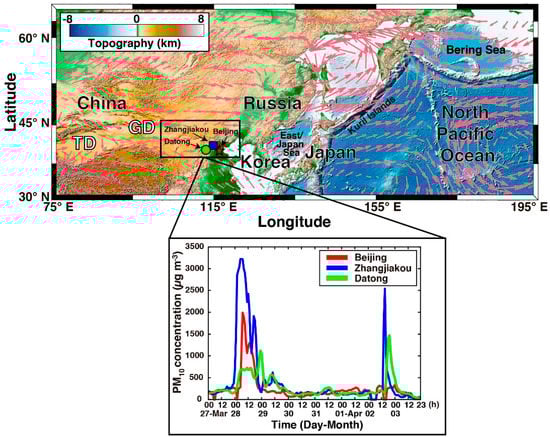
Figure 1.
(Upper figure) Study map illustrating the area of interest from central Asia to the North Pacific Ocean (30° N–65° N and 75° E–195° E). The color scale represents 2-Minute Gridded Global Relief Data (ETOPO2v2) topography. The pink arrows represent surface mean winds during 26 March to 4 April 2018. TD is the Taklimakan desert and GD is the Gobi desert. Red star, blue square, and green circle indicate Beijing (39.91° N, 116.40° E), Zhangjiakou (40.81° N, 114.88° E), and Datong (40.09° N, 113.29° E), respectively. (Lower figure) Hourly mass concentrations of PM10 (μg m−3) in Beijing (red line), Zhangjiakou (blue line), and Datong (green line).
Modeling and observational studies reveal that the supply of Asian dust to the North Pacific Ocean occurs primarily in spring (March–May) by westerly winds [17,20,21]. Several studies have proposed a significant linkage between spring Asian dust events and biological activity in the North Pacific Ocean [6,22,23,24]. Yoon et al. [24] reported that OPP can be increased by more than 70% by dust transport events to the western North Pacific Ocean, compared to dust free periods, suggesting their potential for enhancing biological pumps.
An accurate quantification of the impact of mineral dust, however, is still difficult at both regional and global scales. As the dust particles are transported to long distances from their source regions to the North Pacific Ocean [20,21,25], the crucial factors for examining their impacts on OPP include an accurate understanding of physical processes such as dust sources, dust aerosol types, horizontal and vertical transport pathways, and dust deposition. Recent developments in techniques such as multiple satellite measurements, ground-based observations, and model simulations are capable of monitoring these characteristics of dust events [26,27,28,29]. A few studies, however, have combined the analysis of sources, transport and vertical distribution of Asian dust, and their impacts on ocean biogeochemical cycles in combination by integrating these multiple techniques.
Severe dust events swept over East Asia during 26 March to 4 April 2018. These storms affected 10 provinces, covering an area of ~9.3 × 10⁵ km2, located in northern China, decreasing air quality to hazardous levels (i.e., air quality index > 300; health warnings of emergency conditions), and then moved to the North Pacific Ocean. However, studies on the sources, transport, and vertical distribution of such events, as well as their impacts on OPP in the North Pacific Ocean, are relatively scarce. Therefore, the purpose of this study is (1) to investigate the sources and transport characteristics of recent severe Asian dust events that occurred in spring 2018 using multiple satellite measurements, ground observations, and model simulation, and (2) to examine their potential impacts on the North Pacific OPP.
2. Data and Methods
2.1. Meteorological Measurements
Dust events are associated with increases in PM10 (particulate matter less than 10 μm in diameter) concentrations more than 2-fold, compared to normal atmospheric conditions [30,31,32,33,34]. We used the hourly near-surface PM10 mass concentrations from 27 March to 3 April 2018 at three monitoring stations (Beijing, Zhangjiakou, and Datong) located in northern China (Figure 1) to investigate the occurrence of dust events. The data were collected from the China air quality online monitoring and analysis platform [35].
2.2. Atmospheric Data
In this study, the sources, transport, and aerosol types of the Asian dust events over the North Pacific Ocean from 26 March to 4 April 2018 were comprehensively detected using multi-satellite measurements. First, the daily true color images from the Visible Infrared Imaging Radiometer Suite (VIIRS) instrument onboard the NASA-NOAA’s Suomi National Polar-orbiting Partnership (S-NPP) satellite were analyzed. The presence of dust, which has a distinct yellow-brownish color, was visually confirmed using the NASA’s Worldview [36] (Figure S1). Aerosol indices (AI)—which are a good indicator of the magnitude of atmospheric dust loading—were used to analyze transport pathways [37,38]. Daily AI data (Figure S2) with resolution of 1° × 1° were derived from the Ozone Mapping and Profiler Suite (OMPS), which is also flying onboard S-NPP [39,40]. For this study, severe dust events were defined as having AI values greater than 1.7 [24].
The Cloud-Aerosol Lidar with Orthogonal Polarization (CALIOP) instrument onboard the Cloud-Aerosol Lidar and Infrared Pathfinder Satellite Observation (CALIPSO) satellite [41] provides a vertical distribution of clouds and aerosols. The CALIPSO Level 2 aerosol classification algorithm (version 4) discriminates seven aerosol types: Clean marine, mineral dust, polluted continental/smoke, clean continental, polluted dust, elevated smoke, and dusty marine (i.e., mixtures of mineral dust and marine aerosols) [42]. The CALIPSO aerosol type algorithm works well in classifying mineral dust type, achieving an agreement of 91% with ground-based aerosol measurements [43,44]. We used Level 2 (version 4) CALIPSO aerosol products and vertical feature mask (VFM) data with a horizontal resolution of 5 km and a vertical resolution of 30 m below 8.2 km, 60 m for 8.2–20.2 km, and 180 m for 20.2–30.1 km [26]. To ensure the quality of CALIPSO data, several quality control flags contained in the Level 2 aerosol products were applied following quality assurance procedures [45,46,47], including only data points with uncertainty of extinction coefficient less than 99.9 km−1 and extinction quality control flags with values of 0 or 1. The CALIPSO cloud-aerosol discrimination (CAD) algorithm separates clouds (i.e., positive CAD score) and aerosols (i.e., negative CAD score), providing a measure of the confidence level for the identification of aerosol types (high confidence: |CAD score| ≥ 70, medium confidence: 50 ≤ |CAD score| < 70, low confidence: 20 ≤ |CAD score| < 50, and no confidence: |CAD score| < 20) [48,49]. Therefore, to enable more reliable aerosol identification by reducing the impact of cloud contamination with high confidence levels, we excluded data points with CAD scores > −70 [48,50,51]. Therefore, we used only high confidence data for the analysis of CALIPSO aerosol type classification.
Aerosol optical depth (AOD) is a measure of light extinction (i.e., scattering or absorption) by aerosols in the atmospheric column, and during specific dust outbreaks AOD data are utilized as useful information to characterize the spatial distribution of dust events, especially over oceans [52,53,54]. Daily gridded total AOD at 550 nm from 26 March to 4 April 2018 was provided by the Copernicus Atmosphere Monitoring Service (CAMS) global near-real time analysis system [55], with a spatial resolution of 0.4° × 0.4° latitude-longitude, implemented by European Centre for Medium Range Weather Forecasts (ECMWF).
The HYSPLIT model developed by NOAA’s Air Resources Laboratory was employed to generate air mass backward trajectories for determining the sources of dust events [56]. HYSPLIT backward trajectories have been widely used to track the emission sources of atmospheric pollutants including wind-blown dust [57,58]. HYSPLIT runs are driven by the Global Data Assimilation System (GDAS) with a spatial resolution of 1° × 1° latitude-longitude.
To analyze the synoptic conditions associated with the transportation of Asian dust over the North Pacific Ocean, the surface wind velocity fields of the globally gridded (2.5° × 2.5°) daily wind velocities were taken from the National Centers for Environmental Prediction/National Center for Atmospheric Research (NCEP/NCAR) reanalysis data [59,60].
2.3. Physical and Biological Ocean Data
To investigate the impact of Asian dust events on OPP in the North Pacific Ocean, we first analyzed chlorophyll-a (CHL-a) concentrations, a representative of phytoplankton biomass [61,62]. CHL-a data were derived from VIIRS data with a 4 km spatial resolution and daily temporal resolution [63]. OPP was estimated from the CHL-a based Kameda-Ishizaka model [64]. Input parameters for this model were obtained from VIIRS-derived Level 3 daily CHL-a concentrations, photosynthetic available radiation (E m−2 d−1), sea surface temperature (SST; °C), euphotic depth (Zeu; m), and day length (h). To quantify the potential of Asian dust to increase the biological pump, we also estimated ocean export production (OEP) from three widely-used global satellite models; Dunne07 model [65], Laws11 model [66], and Henson11 model [67], using OPP estimates and VIIRS-derived CHL-a and SST data from above. The response of OPP and OEP to Asian dust was quantified by comparing the current dust condition (2018) vs. the average condition for six years (2012–2017; VIIRS data available since 2012). Dust condition (2018) estimates were calculated by averaging OPP and OEP over a 13-day period (17–29 April) influenced by dust events, and average condition estimates were calculated by averaging the values for the same period for six years.
To investigate the influence of physical dynamic variability on OPP in a local region of the North Pacific Ocean, which exhibited high CHL-a concentrations after the dust events, we also calculated mixed layer depth (MLD) as the depth at which temperature changes by 0.2 °C from the temperature at 3 m reference depth [68]. Daily water temperature data were obtained from the Hybrid Coordinate Ocean Model (HYCOM) with Navy Coupled Ocean Data Assimilation (NCODA) global hindcast analysis based on a 1/12° × 1/12° horizontal resolution and 40 standard vertical levels [69].
3. Results
3.1. Dust Occurrence and Transportation
Severe dust storms over East Asia were analyzed between 26 March and 4 April 2018. These storms caused an increase in PM10 concentrations at least two-fold in comparison with normal atmospheric conditions [28,34,70]. Figure 1 shows the hourly mass concentrations of PM10 in Beijing (39.91° N, 116.40° E), Zhangjiakou (40.81° N, 114.88° E), and Datong (40.09° N, 113.29° E) from 27 March to 3 April 2018.
Hourly PM10 concentrations in Beijing rapidly rose from 190 μg m−3 at local 00:00 on 27 March to a maximum of 1989 μg m−3 at local 07:00 on 28 March; a secondary peak (>300 μg m−3) at local 20:00 on 2 April was observed. The two other stations also show similar variations of PM10 levels, with double peaks exceeding 1000 μg m−3 on 28 March and 2 April. Values exceeded 2500 μg m−3—nearly 25 times than that under normal conditions—in Zhangjiakou, with comparable PM10 concentrations (1500–2000 μg m−3) in May 2017, when an intense dust storm engulfed northern China [71]. These indicate that severe dust events affected northern China on both 28 March and 2 April.
Figure 2 represents the spatial distribution of total AOD at 550 nm derived from CAMS—which indicates atmospheric dust loads during dust events. The high AOD values exceeding 1 were mainly distributed over the Gobi deserts on 26 March (Figure 2a). AOD values showed the subsequent increase from source regions over northern China on 27 March (Figure 2b), over the East/Japan Sea on 28–29 March (Figure 2c–d), and finally over the North Pacific Ocean on 29–31 March (Figure 2d–f). It was likely that the second group of dust storms occurred over the Taklimakan and Gobi deserts on 1–2 April (Figure 2g–h), carrying high atmospheric dust loading from their source regions (AOD > 1). It reached northern China on the 2 April, and then through the East/Japan Sea reached the North Pacific Ocean on 3–4 April (Figure 2h–j). These dust movements revealed by aerosol model images are in agreement with the temporal variations in the ground-based PM10 concentrations (Figure 1).
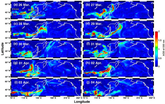
Figure 2.
(a–j) Spatial distributions of total AOD at 550 nm data from CAMS at 12:00 UTC from 26 March to 4 April 2018.
The distribution and transport of the dust plumes that developed over East Asia were also visually inspected as S-NPP VIIRS true color images during 26 March to 3 April 2018 (Figure S1). As the dust storms occurred during 26 March to 4 April were influenced by cloud interferences, VIIRS true color images were overlaid with the satellite AI values as contours lines, indicating dust outbreak and transport. Figure S1a shows that the dust outbreak occurred over the Taklimakan and Gobi deserts on 26 March. The dust plume soon reached to the East/Japan Sea on 28 March (Figure S1b), and then moved to the North Pacific Ocean on 29 March (Figure S1c). Another dust plume originating from the Taklimakan and Gobi deserts was detected on 2 April (Figure S1d). It reached to the North Pacific Ocean on 3 April (Figure S1e).
Satellite-based AI estimates have been widely used as key indicators to determine the source regions of dust events and to trace the pathways along which they are transported [37,72], even over bright backgrounds, such as clouds and snow/ice covered areas, by estimating a pair of radiances in the near UV to detect the presence of absorbing aerosols (i.e., desert dust, biomass burning, and boreal forest fires) [73]. Although the cloud interferences could overestimate the satellite-based AI measurements [73,74,75] during the study period, the cloud interferences on AI estimation were not significant (Text S1 and Table S1). Based on the geographical AI distributions (Figure 3 and Figure S2), the transportation pathways of the Asian dust events (high AI values > 1.7) were consistent with visual true color and AOD images, but showing more distinct geographic distribution. As shown in Figure S1 and Figure 2, high quantities of dust were transported over the North Pacific Ocean during 26 March to 4 April 2018. Figure 3 shows the spatial distribution of the AI values averaged for each event: 26–31 March (Figure 3a) and 1–4 April (Figure 3b).
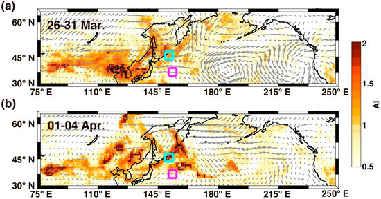
Figure 3.
Spatial distributions of AI for (a) 26–31 March and (b) 1–4 April 2018 in the North Pacific Ocean. The grey arrows represent mean surface wind velocities averaged over 4–6 days spanning dust events. The cyan square (45° N–46° N and 151° E–152° E) indicates 1° × 1° region in which AI exceeded the 1.7 threshold value on both events, while the pink square (37° N–38° N and 153° E–154° E) indicates 1° × 1° region in which AI values were less than 1. Data from the two areas were used for OPP estimation (refer to Section 4.2).
The two dust storms moved eastward from desert source regions through the East/Japan Sea to the North Pacific Ocean. However, they exhibited different transportation pathways from northern China to the North Pacific Ocean; the first moved northeast into the Bering Sea while the other moved east along 42° N. These patterns appear to be dependent upon the direction of the westerly winds [18,24]. The first dust event occurred on 26–27 March (Figure S2a,b); the southwesterly winds caused the dust plume to shape into a narrow band (AI > 1.7) that moved northeastward, passing over the northern East/Japan Sea and the Okhotsk Sea on 28 March (Figure S2c). On 29 March, the dust plume was transported over the southern East/Japan Sea and Kuril Islands by stronger southwesterly winds, from whence it was spread into the Bering Sea on 29–31 March by strong southerly winds (Figure S2d–f). On the other hand, the second dust event that occurred on 1 April was lofted over the East/Japan Sea and Kuril Islands by westerly winds, showing high AI values > 2.0 (Figure 3b and Figure S2g–j).
3.2. Tracing Dust Source Regions Using Backward Trajectory
To investigate the sources of dust storms over the North Pacific Ocean, the HYSPLIT model was used to track the movements of air masses that reached the North Pacific Ocean during the relevant time frame. Figure 4 shows the backward trajectories of air masses at a point located around the Kuril Islands (47.52° N, 152.67° E; black star in Figure 4) along the transport pathways of two dust events at 12:00 UTC on 29 March and 12:00 UTC on 3 April 2018, respectively. The duration of the trajectories was 36 h at 6-h intervals, and the arriving altitudes of the air masses were 5000, 6000, and 7000 m. The backward trajectories also support the dust source regions and transport pathways revealed by the analyses of satellite-based AI estimates and VIIRS true color images (Figure 3, Figures S1 and S2). The 72-h backward trajectories from the Bering Sea (60.71° N, 177.15° W; black star in Figure S3) ending at 12:00 UTC on 30 March at altitudes of 5000, 6000, and 7000 m also show that the dust storm from the Taklimakan and Gobi deserts moved through the Kuril Islands on 29 March into the Bering Sea on 30 March. This was in concordance with the OMPS observations.

Figure 4.
Back trajectories derived from the NOAA HYSPLIT model at different altitude levels (5000, 6000, 7000 m; red line, blue line, green line, respectively) at a point around the Kuril Islands (black star; 47.52° N, 152.67° E) on (a) 12:00 UTC 29 March 2018 and (b) 12:00 UTC 3 April 2018. The inset figures indicate the back trajectories at 7000 m overlaid onto Figure 3a and b, respectively.
3.3. Vertical Distribution of Dust Composition and Extinction Coefficient
To confirm that the high AI values (AI > 1.7) were caused by mineral dust aerosols along transport pathways from the Taklimakan and Gobi deserts to the North Pacific Ocean, the vertical distributions of aerosol types and dust extinction coefficients at 532 nm from CALIPSO observations were analyzed. Figure 5 depicts the vertical distributions of the aerosol types along CALIPSO orbit paths (Figure 5a), covering the dust source regions, northern China, the East/Japan Sea, and the North Pacific Ocean. The high AI value regions (Figure 3 and Figure S2) were dominated by mineral dust aerosols (orange-shaded areas in Figure 5), indicating the transport of mineral dust over the North Pacific Ocean from the Taklimakan and Gobi deserts during 26 March to 4 April 2018. Furthermore, aerosol types classified by CALIPSO measurements indicated that mineral dust aerosols were vertically dominant in the altitudes of 2–7 km in the Gobi desert (Figure 5b,e–f), and then moved to the North Pacific Ocean (Figure 5c,d,g,h) ascending to 3–10 km. Mineral dust aerosols make up ~60% of total aerosols between 27 March and 4 April 2018 (Figure S4). In the land, polluted dust and smokes aerosols were mainly distributed out of Gobi desert (Figure 5b,e–f). In the ocean, the marine aerosols, including clean marine aerosols and dusty marine aerosols, were found below 3 km altitude (Figure 5c,d,g,h).
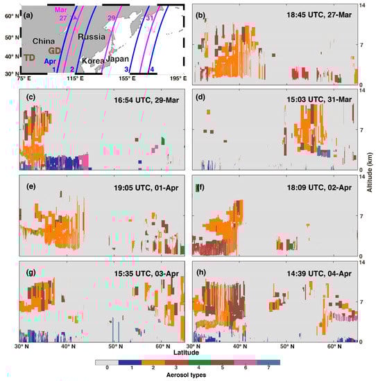
Figure 5.
(a) CALIPSO satellite orbit paths (pink lines on March and blue lines on April); (b–h) Vertical profiles of CALIPSO aerosol types along orbit paths shown in Figure 5a. Color bar indicates aerosol types defined as not determined (0), clean marine (1), mineral dust (2), polluted continental/smoke (3), clean continental (4), polluted dust (5), elevated smoke (6), and dusty marine (7).
Based on the aerosol type classification information derived from CALIPSO, Figure 6 shows the vertical distributions of dust extinction coefficients at 532 nm (i.e., extinction coefficients at 532 nm for mineral dust aerosols) along the same orbit paths as in Figure 5 (Figure 6a). The extinction coefficient of mineral dust represents the amount of mineral dust aerosols in the atmosphere [76,77,78]. The non-dust aerosol extinction coefficient is set to 0.0 km−1. The dust aerosol extinctions in the Gobi desert show a dense deep dust layer (>0.1 km−1) for 2–5 km at 18:45 UTC on 27 March and 19:05 UTC on 1 April (Figure 6b,e), confirming the emissions from the source regions. The high dust extinction coefficients for 2–5 km were also found over northern China, even in the downwind region, the East/Japan Sea (Figure 6c,f), indicating relatively dense dust plumes at low altitude. A dense thin layer was located near 3.5 km in the North Pacific Ocean on 3–4 April (Figure 6g–h), whereas relatively lower extinction coefficients were observed on 31 March (Figure 6d), indicating relatively denser mineral dust loads on 3–4 April compared to 31 March in the North Pacific Ocean.
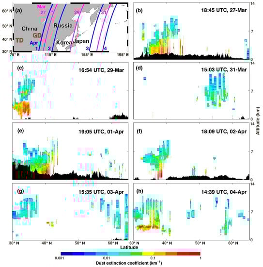
Figure 6.
(a) CALIPSO satellite orbit paths (pink lines on March and blue lines on April); (b–h) Vertical profiles of the CALIPSO dust extinction coefficients at 532 nm (km−1) along orbit paths shown in Figure 6a.
4. Discussion
4.1. Uncertainties of the Atmospheric Data
In previous studies, during Asian dust events, considerable increases in iron depositions were observed in the Yellow Sea and Korean peninsula [79,80,81,82]. As the Western North Pacific Ocean focused upon in the present study is located downwind from the source regions of Asian dust, it implies that iron supply may have increased in the study area via the Asian dust events. Thus, it is likely to be reasonable to hypothesize that OPP in the study area will/may be affected by these dust events.
However, there are some caveats associated with the linkage between Asian dust events and OPP. Firstly, various satellite and model data used in this study do not provide quantitative information about dust depositions onto the study area [83,84,85], suggesting that high AI values are not necessarily associated with high iron deposition rates [54,86,87]. Secondly, iron solubility, which is an important consideration in assessing the impact of dust depositions on OPP [88,89], may be different according to the aerosol source types and deposition mode [90,91,92,93,94]. It was reported that iron solubility was widely ranged from ~1 to 49% during the dust events in the North Pacific Ocean [95,96,97,98,99]. However, we could not resolve two caveats via the present satellite analysis, suggesting that in-situ measurements on dust deposition and iron solubility are needed in future study. Therefore, we note that in the following section, increase of OPP in response to the Asian dust events is likely to be potential.
4.2. Potential Response of OPP to Dust Events
To quantitatively estimate the potential enhancement in the North Pacific OPP to these events, we first compared the temporal analysis of CHL-a concentrations in two smaller areas: Dust-affected area (45° N–46° N and 151° E–152° E, cyan square in Figure 3b) vs. area with no dust (37° N–38° N and 153° E–154° E, pink square in Figure 3b). The dust-affected area was an area where AI values exceeded the threshold 1.7 for both events; 1.9 on 29 March and 2.5 on 3 April, respectively, while AI values were less than 1 in the area with no dust, indicating that this area was not significantly affected by the spring 2018 Asian dust events. The CHL-a patterns of two areas showed different temporal features (Figure 7a,b). In the dust-affected area (Figure 7a), CHL-a doubled from the mean value of 0.4 mg m−3 on April 17 with a lag time of 14 days after the dust event on 3 April (AI = 2.5), and showed a peak (maximum: 3.8 mg m−3 on 29 April). The increase was maintained for ~13 days (see the shadow zone in Figure 7a). On the other hand, in the area with no dust (Figure 7b), the concentration of CHL-a was consistent over time (<1 mg m−3) and was similar to the mean values (0.3 mg m−3) averaged for values from March to April in 2012–2017 (covering the period available from VIIRS) (Figure 7b). This result is consistent with previous studies that North Pacific OPP was dramatically stimulated by Asian dust with a lag of ~10 days [6,23,24]. Such a lag time is attributed to complex factors, such as the dissolution process of iron deposited to the oceans, the physiological and biochemical adaptation of phytoplankton to iron supply in surface waters, and phytoplankton community composition [100,101,102,103,104,105,106,107].
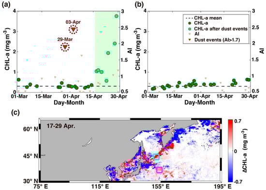
Figure 7.
Daily AI values (triangles) and daily CHL-a concentrations (mg m−3, circles) during the 2018 spring in (a) dust-affected area (cyan square in Figure 7c), (b) area with no dust (pink square in Figure 7c) in the North Pacific Ocean. The black dotted line indicates mean CHL-a concentrations averaged for values from March to April in 2012–2017. The green shading highlights enhanced CHL-a feature driven by strong spring Asian dust. (c) Spatial distributions of ΔCHL-a (mg m−3) for 17–29 April 2018.
The second step in the investigation involved the analysis of the spatial distribution of CHL-a anomalies with a lag of 14 days after the onset of the dust event. CHL-a anomalies (ΔCHL-a) assumed to represent the CHL-a response to dust events were defined as ΔCHL-a(2018) = CHL-a(2018) − CHL-a(mean), where CHL-a(2018) is the CHL concentration for 2018 defined as the composite over a 13-day period (17–29 April), beginning with a lag of 14 days after the onset of the Asian dust event on 3 April 2018; CHL-a(mean) is the mean CHL-a concentration averaged over the same period between 2012 and 2017. Figure 7c shows that the spatial distribution of positive CHL-a anomalies (i.e., ΔCHL-a > 0) in 2018 appeared generally consistent with the overall distribution of AI values > 1.7 (Figure 3). However, a future study, based on in-situ observation, is needed to elucidate the direct link between high AI vales and positive CHL-a anomalies as cause and effect in the dust-affected areas.
Furthermore, to quantify the potential increases in the biological carbon pump in the North Pacific Ocean through these spring 2018 Asian dust events, we estimated satellite-based OPP and OEP (Table S2) by comparing the dust condition (2018) vs. the average condition for six years (2012–2017). OPP and OEP for dust condition were calculated for composites over a 13-day period (17–29 April 2018), while the average condition was calculated for the composites over the same 13-day period between 2012 and 2017. Our analysis suggests that OPP was increased by 48% after those spring 2018 dust events (381 ± 151 mg C m−2 d−1) as compared to the average values for 6 years (258 ± 30 mg C m−2 d−1). Ocean export production estimated using the three models (Dunne07 model [65], Laws11 model [66], and Henson11 model [67]), was in the range from 77 to 164 mg C m−2 d−1 in 2018, while it ranged between 51 and 79 mg C m−2 d−1 (the average range for the 6 years).
During the spring 2018 dust events, positive CHL-a anomaly areas were distributed around the Kuril Islands (Figure 7c), which are known as the area with strong physical mixing occurring [108,109,110], leading to supply of nutrients to the surface waters for phytoplankton growth. To examine the influence of physical mixing on CHL-a variation in the area, we analyzed non-dust spring 2017 CHL-a and MLD data in the same area represented in the present study (see blue square in Figure 7c, showing AI > 1.7 that indicates the occurrence of a dust event) (Figure S5). Daily CHL-a concentrations during the spring (from 1 March to 30 April) 2017 were quite constant, consistent to the climatological mean concentration (Figure S5a). In addition, MLD variation in spring 2017 was comparable with spring 2018, except in 4 April 2017 it was showing abrupt decreasing MLD (Figure S5b). However, there was an episodic enhancement of CHL-a concentrations in the area during spring 2018 (Figure 7a), compared to the climatological trend which is typical bloom associated with the shoaling of MLD. These results support the hypothesis that the observed increase in CHL-a in the area may be associated with the spring 2018 Asian dust events. Therefore, Asian dust events can be regarded as a potential driver for enhancing OPP in the North Pacific Ocean, though short periods.
5. Summary and Conclusions
To understand the comprehensive characteristics of the sources, transport, and impact on OPP of the severe Asian dust events that occurred during 26 March to 4 April 2018, we combined multiple satellite observations, ground-based measurements, and model simulations. We found that two severe dust events influenced northern China near the desert source regions, with double peaks of PM10 mass concentrations reaching up to 3000 μg m−3 on 28 March and 2 April.
Satellite AI data indicated that the two events originated from the Taklimakan and Gobi deserts, moved eastward through the East/Japan Sea and into the North Pacific Ocean. However, two dust events showed different transportation pathways from northern China over the North Pacific Ocean; one moved northeast into the Bering Sea and the other moved east along 42° N. Furthermore, aerosol types classified using CALIPSO satellite data indicated that the two dust events originating from the Taklimakan and Gobi deserts were dominated by mineral dust aerosols at altitudes of 2–7 km with a dense deep layer of 2–5 km and were transported over the North Pacific Ocean ascending to 3–10 km, at the relatively denser dust plumes on the second dust episode than the first. We compared the time series of CHL-a concentrations in two smaller areas: Dust-affected area vs. area with no dust. The CHL-a values after strong dust events in the dust-affected area were increased 3-fold compared to that in the area with no dust. These and other results suggest that mineral dust emitted from the Taklimakan and Gobi deserts could increase ocean productivity by ~50% in the effected regions, emphasizing that the Asian dust event could have a potential impact for enhancing the ocean biological pump by supplying scarce bioavailable iron to the North Pacific Ocean.
Supplementary Materials
The following are available online at https://www.mdpi.com/2073-4433/10/5/276/s1, Text S1. The influence of cloud interferences on AI estimates. Table S1: Comparison of AI values for green boxes (cloud-free condition) and blue boxes (cloud-covered condition) shown in Figure S1. Table S2: OPP (mg C m−2 d−1) and OEP (mg C m−2 d−1) estimates averaged over a 13-day period (17–29 April) in 2018 and mean values averaged over the same period between 2012 and 2017. Data were averaged for the dust-affected area (blue square) shown in Figure 7c. Figure S1: (a–e) The S-NPP VIIRS true color images for 26, 28–29 March and 2–3 April 2018. Black dotted box indicates the dust outbreak and transport recognized as a yellow-brownish color, and it was overlaid with the AI values as contour lines. TD is the Taklimakan desert and GD is the Gobi desert. Green boxes indicate cloud-free conditions, and blue boxes indicate cloud-covered conditions. Figure S2: (a–j) Spatial distributions of AI from 26 March to 4 April 2018. The grey arrows represent daily surface wind vectors. Figure S3: Back trajectories derived from the NOAA HYSPLIT model at different altitude levels (5000, 6000, 7000 m; red line, blue line, green line, respectively) in Bering Sea (black star; 60.71° N, 177.15° W) on 12:00 UTC 30 March 2018. The inset figure indicates the back trajectory at 7000 m overlaid onto Figure 3a. Figure S4: Pie chart of the mean composition of aerosols types along orbit paths shown in Figure 5a. Color bar indicates aerosol types defined as clean marine (1), mineral dust (2), polluted continental/smoke (3), clean continental (4), polluted dust (5), elevated smoke (6), and dusty marine (7). Figure S5: (a) Daily AI values (triangles) and daily CHL-a concentrations (mg m−3, circles) during the 2017 spring for the area marked as a cyan square in Figure 7c. The black dotted line indicates mean CHL-a concentrations averaged for values from March to April in 2012–2017. (b) Daily MLD during the 2017/2018 spring in cyan square in Figure 7c.
Author Contributions
Conceptualization, J.-E.Y. and I.-N.K.; methodology, J.-E.Y. and I.-N.K.; software, J.-E.Y.; validation, J.-E.Y.; formal analysis, J.-E.Y.; investigation, J.-E.Y.; resources, J.-E.Y.; data curation, J.-E.Y.; writing—original draft preparation, J.-E.Y. and I.-N.K.; writing—review and editing, J.-E.Y., I.-N.K., J.-H.L., J.-M.S., and J.-I.K.; visualization, J.-E.Y.; supervision, I.-N.K.; project administration, I.-N.K.; funding acquisition, I.-N.K.
Funding
This work was supported by Incheon National University Research Grant in 2016.
Acknowledgments
We thank product developers of VIIRS, OMPS, CALIPSO satellites, and CAMS, HYCOM, HYSPLIT model for free sharing of products.
Conflicts of Interest
The authors declare no conflict of interest.
References
- Martin, J.H. Glacial-interglacial CO2 change: The iron hypothesis. Paleoceanography 1990, 5, 1–13. [Google Scholar] [CrossRef]
- Boyd, P.W. Mesoscale iron enrichment experiments 1993–2005: Synthesis and future directions. Science 2007, 315, 612–617. [Google Scholar] [CrossRef] [PubMed]
- Taylor, S.R. Abundance of chemical elements in the continental crust: A new table. Geochim. Cosmochim. Acta 1964, 28, 1273–1285. [Google Scholar] [CrossRef]
- Gordon, R.M.; Martin, J.H.; Knauer, G.A. Iron in North-East Pacific Waters. Nature 1982, 299, 611–612. [Google Scholar] [CrossRef]
- Martin, J.H.; Fitzwater, S.E. Iron deficiency limits phytoplankton growth in the North-East Pacific Subarctic. Nature 1988, 331, 341–343. [Google Scholar] [CrossRef]
- Bishop, J.K.B.; Davis, R.E.; Sherman, J.T. Robotic observations of dust storm enhancement of carbon biomass in the North Pacific. Science 2002, 298, 817–821. [Google Scholar] [CrossRef]
- Boyd, P.W.; Mackie, D.S.; Hunter, K.A. Aerosol iron deposition to the surface ocean—modes of iron supply and biological responses. Mar. Chem. 2010, 120, 128–143. [Google Scholar] [CrossRef]
- Kohfeld, K.E.; Harrison, S.P. Dirtmap: The geological record of dust. Earth Sci. Rev. 2001, 54, 81–114. [Google Scholar] [CrossRef]
- Bopp, L.; Kohfeld, K.E.; Le Quere, C.; Aumont, O. Dust impact on marine biota and atmospheric CO2 during glacial periods. Paleoceanography 2003, 18. [Google Scholar] [CrossRef]
- Blain, S.; Queguiner, B.; Armand, L.; Belviso, S.; Bombled, B.; Bopp, L.; Bowie, A.; Brunet, C.; Brussaard, C.; Carlotti, F.; et al. Effect of natural iron fertilization on carbon sequestration in the Southern Ocean. Nature 2007, 446, 1070–1074. [Google Scholar] [CrossRef]
- Zender, C.S.; Miller, R.L.R.L.; Tegen, I. Quantifying mineral dust mass budgets: Terminology, constraints, and current estimates. Eos Trans. AGU 2004, 85, 509–512. [Google Scholar] [CrossRef]
- Tanaka, T.Y.; Chiba, M. A numerical study of the contributions of dust source regions to the global dust budget. Glob. Planet. Chang. 2006, 52, 88–104. [Google Scholar] [CrossRef]
- Tegen, I.; Schepanski, K. The global distribution of mineral dust. IOP Conf. Ser. Earth Environ. Sci. 2009, 7, 012001. [Google Scholar] [CrossRef]
- Moore, J.K.; Doney, S.C.; Glover, D.M.; Fung, I.Y. Iron cycling and nutrient-limitation patterns in surface waters of the world ocean. Deep Sea Res. Part. II 2002, 49, 463–507. [Google Scholar] [CrossRef]
- Liu, H.; Suzuki, K.; Saito, H. Community structure and dynamics of phytoplankton in the Western Subarctic Pacific Ocean: A synthesis. J. Oceanogr. 2004, 60, 119–137. [Google Scholar] [CrossRef]
- Krishnamurthy, A.; Moore, J.K.; Zender, C.S.; Luo, C. Effects of atmospheric inorganic nitrogen deposition on ocean biogeochemistry. J. Geophys. Res. 2007, 112, G02019. [Google Scholar] [CrossRef]
- Duce, R.A.; Unni, C.K.; Ray, B.J.; Prospero, J.M.; Merrill, J.T. Long-range atmospheric transport of soil dust from Asia to the tropical North Pacific: Temporal variability. Science 1980, 209, 1522–1524. [Google Scholar] [CrossRef]
- Zhao, T.L.; Gong, S.L.; Zhang, X.Y.; McKendry, I.G. Modeled size-segregated wet and dry deposition budgets of soil dust aerosol during ACE-Asia 2001: Implications for trans-pacific transport. J. Geophys. Res. Atmos. 2003, 108, 8665. [Google Scholar] [CrossRef]
- Ke-Yi, C. The northern path of asian dust transport from the gobi desert to north america. Atmos. Ocean. Sci. Lett. 2010, 3, 155–159. [Google Scholar] [CrossRef]
- Uematsu, M.; Duce, R.A.; Prospero, J.M.; Chen, L.; Merrill, J.T.; McDonald, R.L. Transport of mineral aerosol from Asia over the North Pacific Ocean. J. Geophys. Res. 1983, 88, 5343–5352. [Google Scholar] [CrossRef]
- Takemura, T.; Uno, I.; Nakajima, T.; Higurashi, A.; Sano, I. Modeling study of long-range transport of asian dust and anthropogenic aerosols from east Asia. Geophys. Res. Lett. 2002, 29, 2148. [Google Scholar] [CrossRef]
- Tan, S.-C.; Yao, X.; Gao, H.-W.; Shi, G.-Y.; Yue, X. Variability in the correlation between Asian dust storms and chlorophyll a concentration from the north to equatorial pacific. PLoS ONE 2013, 8, e57656. [Google Scholar] [CrossRef] [PubMed]
- Han, Y.; Zhao, T.; Song, L.; Fang, X.; Yin, Y.; Deng, Z.; Wang, S.; Fan, S. A linkage between asian dust, dissolved iron and marine export production in the deep ocean. Atmos. Environ. 2011, 45, 4291–4298. [Google Scholar] [CrossRef]
- Yoon, J.E.; Kim, K.; Macdonald, A.M.; Park, K.T.; Kim, H.C.; Yoo, K.C.; Yoon, H.I.; Yang, E.J.; Jung, J.; Lim, J.H.; et al. Spatial and temporal variabilities of spring Asian dust events and their impacts on chlorophyll-A concentrations in the western North Pacific Ocean. Geophys. Res. Lett. 2017, 44, 1474–1482. [Google Scholar] [CrossRef]
- Uno, I.; Eguchi, K.; Yumimoto, K.; Takemura, T.; Shimizu, A.; Uematsu, M.; Liu, Z.; Wang, Z.; Hara, Y.; Sugimoto, N. Asian dust transported one full circuit around the globe. Nat. Geosci. 2009, 2, 557–560. [Google Scholar] [CrossRef]
- Winker, D.M.; Hunt, W.H.; McGill, M.J. Initial performance assessment of CALIOP. Geophys. Res. Lett. 2007, 34, L19803. [Google Scholar] [CrossRef]
- Yu, Y.; Kalashnikova, O.V.; Garay, M.J.; Notaro, M. Climatology of asian dust activation and transport potential based on misr satellite observations and trajectory analysis. Atmos. Chem. Phys. 2019, 19, 363–378. [Google Scholar] [CrossRef]
- Tsedendamba, P.; Dulam, J.; Baba, K.; Hagiwara, K.; Noda, J.; Kawai, K.; Sumiya, G.; McCarthy, C.; Kai, K.; Hoshino, B. Northeast asian dust transport: A case study of a dust storm event from 28 March to 2 April 2012. Atmosphere 2019, 10, 69. [Google Scholar] [CrossRef]
- Kim, S.-W.; Yoon, S.-C.; Kim, J.; Kang, J.-Y.; Sugimoto, N. Asian dust event observed in Seoul, Korea, during 29–31 May 2008: Analysis of transport and vertical distribution of dust particles from lidar and surface measurements. Sci. Total Environ. 2010, 408, 1707–1718. [Google Scholar] [CrossRef]
- Fu, Q.; Zhuang, G.; Li, J.; Huang, K.; Wang, Q.; Zhang, R.; Fu, J.; Lu, T.; Chen, M.; Wang, Q.; et al. Source, Long-Range transport, and characteristics of a heavy dust pollution event in Shanghai. J. Geophys. Res. Atmos. 2010, 115. [Google Scholar] [CrossRef]
- Zhao, T.L.; Gong, S.L.; Zhang, X.Y.; Jaffe, D.A. Asian dust storm influence on north American ambient pm levels: Observational evidence and controlling factors. Atmos. Chem. Phys. 2008, 8, 2717–2728. [Google Scholar] [CrossRef]
- Jugder, D.; Shinoda, M.; Kimura, R.; Batbold, A.; Amarjargal, D. Quantitative analysis on windblown dust concentrations of PM10 (PM2.5) during dust events in Mongolia. Aeolian Res. 2014, 14, 3–13. [Google Scholar] [CrossRef]
- Jugder, D.; Shinoda, M.; Sugimoto, N.; Matsui, I.; Nishikawa, M.; Park, S.-U.; Chun, Y.-S.; Park, M.-S. Spatial and temporal variations of dust concentrations in the gobi desert of Mongolia. Glob. Planet. Chang. 2011, 78, 14–22. [Google Scholar] [CrossRef]
- Wang, S.; Yuan, W.; Shang, K. The impacts of different kinds of dust events on PM10 pollution in northern China. Atmos. Environ. 2006, 40, 7975–7982. [Google Scholar] [CrossRef]
- China Air Quality Online Monitoring and Analysis Platform. Available online: https://www.aqistudy.cn/ (accessed on 29 March 2019).
- NASA Worldview. Available online: https://worldview.earthdata.nasa.gov (accessed on 29 March 2019).
- Herman, J.R.; Bhartia, P.K.; Torres, O.; Hsu, C.; Seftor, C.; Celarier, E. Global distribution of UV-absorbing aerosols from Nimbus 7/TOMS data. J. Geophys. Res. 1997, 102, 16911–16922. [Google Scholar] [CrossRef]
- Torres, O.; Tanskanen, A.; Veihelmann, B.; Ahn, C.; Braak, R.; Bhartia, P.K.; Veefkind, P.; Levelt, P. Aerosols and surface UV products from ozone monitoring instrument observations: An overview. J. Geophys. Res. 2007, 112, D24S47. [Google Scholar] [CrossRef]
- NASA EARTHDATA. Available online: https://earthdata.nasa.gov (accessed on 29 March 2019).
- Flynn, L.; Long, C.; Wu, X.; Evans, R.; Beck, C.T.; Petropavlovskikh, I.; McConville, G.; Yu, W.; Zhang, Z.; Niu, J.; et al. Performance of the ozone mapping and profiler suite (OMPS) products. J. Geophys. Res. Atmos. 2014, 119, 6181–6195. [Google Scholar] [CrossRef]
- Cloud-Aerosol Lidar and Infrared Pathfinder Satellite Observation (CALIPSO) Data and Information. Available online: https://eosweb.larc.nasa.gov/project/calipso/calipso_table (accessed on 29 March 2019).
- Kim, M.H.; Omar, A.H.; Tackett, J.L.; Vaughan, M.A.; Winker, D.M.; TreParte, C.R.; Hu, Y.; Liu, Z.; Poole, L.R.; Pitts, M.C.; et al. The calipso version 4 automated aerosol classification and lidar ratio selection algorithm. Atmos. Meas. Tech. 2018, 11, 6107–6135. [Google Scholar] [CrossRef]
- Mielonen, T.; Arola, A.; Komppula, M.; Kukkonen, J.; Koskinen, J.; de Leeuw, G.; Lehtinen, K.E.J. Comparison of caliop level 2 aerosol subtypes to aerosol types derived from aeronet inversion data. Geophys. Res. Lett. 2009, 36, L18804. [Google Scholar] [CrossRef]
- Burton, S.P.; Ferrare, R.A.; Vaughan, M.A.; Omar, A.H.; Rogers, R.R.; Hostetler, C.A.; Hair, J.W. Aerosol classification from airborne HSRL and comparisons with the calipso vertical feature mask. Atmos. Meas. Tech. 2013, 6, 1397–1412. [Google Scholar] [CrossRef]
- Lu, X.; Mao, F.Y.; Pan, Z.X.; Gong, W.; Wang, W.; Tian, L.Q.; Fang, S.H. Three-dimensional physical and Optical characteristics of aerosols over central China from long-term CALIPSO and HYSPLIT data. Remote Sens. 2018, 10, 314. [Google Scholar] [CrossRef]
- Tackett, J.L.; Winker, D.M.; Getzewich, B.J.; Vaughan, M.A.; Young, S.A.; Kar, J. Calipso lidar level 3 aerosol profile product: Version 3 algorithm design. Atmos. Meas. Tech. 2018, 11, 4129–4152. [Google Scholar] [CrossRef]
- Winker, D.M.; Tackett, J.L.; Getzewich, B.J.; Liu, Z.; Vaughan, M.A.; Rogers, R.R. The global 3-D distribution of tropospheric aerosols as characterized by CALIOP. Atmos. Chem. Phys. 2013, 13, 3345–3361. [Google Scholar] [CrossRef]
- Liu, Z.; Vaughan, M.A.; Winker, D.M.; Hostetler, C.A.; Poole, L.R.; Hlavka, D.; Hart, W.; McGill, M. Use of probability distribution functions for discriminating between cloud and aerosol in lidar backscatter data. J. Geophys. Res. Atmos. 2004, 109, D15202. [Google Scholar] [CrossRef]
- Liu, Z.; Kar, J.; Zeng, S.; Tackett, J.; Vaughan, M.; Avery, M.; Pelon, J.; Getzewich, B.; Lee, K.P.; Magill, B.; et al. Discriminating between clouds and aerosols in the CALIOP version 4.1 data products. Atmos. Meas. Tech. 2019, 12, 703–734. [Google Scholar] [CrossRef]
- Yang, W.; Marshak, A.; Várnai, T.; Liu, Z. Effect of calipso cloud–aerosol discrimination (CAD) confidence levels on observations of aerosol properties near clouds. Atmos. Res. 2012, 116, 134–141. [Google Scholar] [CrossRef]
- Liu, Z.; Vaughan, M.; Winker, D.; Kittaka, C.; Getzewich, B.; Kuehn, R.; Omar, A.; Powell, K.; TreParte, C.; Hostetler, C. The calipso lidar cloud and aerosol discrimination: Version 2 algorithm and initial assessment of performance. J. Atmos. Ocean. Technol. 2009, 26, 1198–1213. [Google Scholar] [CrossRef]
- Ginoux, P.; Chin, M.; Tegen, I.; Prospero, J.M.; Holben, B.; Dubovik, O.; Lin, S.-J. Sources and distributions of dust aerosols simulated with the gocart model. J. Geophys. Res. Atmos. 2001, 106, 20255–20273. [Google Scholar] [CrossRef]
- Grousset, F.E.; Ginoux, P.; Bory, A.; Biscaye, P.E. Case study of a chinese dust plume reaching the french alps. Geophys. Res. Lett. 2003, 30, 1277. [Google Scholar] [CrossRef]
- Mahowald, N.; Engelstaedter, S.; Luo, C.; Sealy, A.; Artaxo, P.; Benitez-Nelson, C.; Bonnet, S.; Chen, Y.; Chuang, P.; Cohen, D.D.; et al. Atmospheric iron deposition: Global distribution, variability, and human perturbations. Ann. Rev. Mar. Sci. 2009, 1, 245–278. [Google Scholar] [CrossRef]
- Copernicus Atmosphere Monitoring Service. Available online: http://atmosphere.copernicus.eu (accessed on 29 March 2019).
- NOAA Air Resources Laboratory. Available online: https://www.arl.noaa.gov/hysplit/hysplit/ (accessed on 29 March 2019).
- Fleming, Z.L.; Monks, P.S.; Manning, A.J. Review: Untangling the influence of Air-Mass history in interpreting observed atmospheric composition. Atmos. Res. 2012, 104–105, 1–39. [Google Scholar] [CrossRef]
- Stein, A.F.; Draxler, R.R.; Rolph, G.D.; Stunder, B.J.B.; Cohen, M.D.; Ngan, F. NOAA’S HYSPLIT atmospheric transport and dispersion modeling system. Bull. Am. Meteorol. Soc. 2015, 96, 2059–2077. [Google Scholar] [CrossRef]
- Kalnay, E.; Kanamitsu, M.; Kistler, R.; Collins, W.; Deaven, D.; Gandin, L.; Iredell, M.; Saha, S.; White, G.; Woollen, J.; et al. The NCEP/NCAR 40-year reanalysis project. Bull. Am. Meteorol. Soc. 1996, 77, 437–472. [Google Scholar] [CrossRef]
- Kistler, R.; Kalnay, E.; Collins, W.; Saha, S.; White, G.; Woollen, J.; Chelliah, M.; Ebisuzaki, W.; Kanamitsu, M.; Kousky, V.; et al. The NCEP–NCAR 50-year reanalysis: Monthly means CD-ROM and documentation. Bull. Am. Meteorol. Soc. 2001, 82, 247–268. [Google Scholar] [CrossRef]
- Steele, J.H. Environmental control of photosynthesis in the sea. Limnol. Oceanogr. 1962, 7, 137–150. [Google Scholar] [CrossRef]
- Cullen, J.J. The deep chlorophyll maximum: Comparing vertical profiles of Chlorophyll a. Can. J. Fish. Aquat. Sci. 1982, 39, 791–803. [Google Scholar] [CrossRef]
- NASA OceanColor Web. Available online: http://oceancolor.gsfc.nasa.gov (accessed on 29 March 2019).
- Kameda, T.; Ishizaka, J. Size-fractionated primary production estimated by a two-phytoplankton community model applicable to ocean color remote sensing. J. Oceanogr. 2005, 61, 663–672. [Google Scholar] [CrossRef]
- Dunne, J.P.; Sarmiento, J.L.; Gnanadesikan, A. A synthesis of global particle export from the surface ocean and cycling through the ocean interior and on the seafloor. Glob. Biogeochem. Cycles 2007, 21. [Google Scholar] [CrossRef]
- Laws, E.A.; D’Sa, E.; Naik, P. Simple equations to estimate ratios of new or export production to total production from satellite-derived estimates of sea surface temperature and primary production. Limnol. Oceanogr. 2011, 9, 593–601. [Google Scholar] [CrossRef]
- Henson, S.A.; Sanders, R.; Madsen, E.; Morris, P.J.; Le Moigne, F.; Quartly, G.D. A reduced estimate of the strength of the ocean’s biological carbon pump. Geophys. Res. Lett. 2011, 38, L04606. [Google Scholar] [CrossRef]
- Thompson, R.O.R.Y. Climatological numerical models of the surface mixed layer of the ocean. J. Phys. Oceanogr. 1976, 6, 496–503. [Google Scholar] [CrossRef]
- Hybrid Coordinate Ocean Model (HYCOM). Available online: https://www.hycom.org/data/glbu0pt08/expt-91pt2 (accessed on 29 March 2019).
- Zhang, X.X.; Sharratt, B.; Chen, X.; Wang, Z.F.; Liu, L.Y.; Guo, Y.H.; Li, J.; Chen, H.S.; Yang, W.Y. Dust deposition and ambient PM10 concentration in northwest China: Spatial and temporal variability. Atmos. Chem. Phys. 2017, 17, 1699–1711. [Google Scholar] [CrossRef]
- Song, P.; Fei, J.; Li, C.; Huang, X. Simulation of an asian dust storm event in May 2017. Atmosphere 2019, 10, 135. [Google Scholar] [CrossRef]
- Prospero, J.M.; Ginoux, P.; Torres, O.; Nicholson, S.E.; Gill, T.E. Environmental characterization of global sources of atmospheric soil dust identified with the nimbus 7 total ozone mapping spectrometer (TOMS) absorbing aerosol product. Rev. Geophys. 2002, 40, 2:1–2:31. [Google Scholar] [CrossRef]
- Torres, O.; Jethva, H.; Bhartia, P.K. Retrieval of aerosol optical depth above clouds from OMI observations: Sensitivity analysis and case studies. J. Atmos. Sci. 2012, 69, 1037–1053. [Google Scholar] [CrossRef]
- Ahn, C.; Torres, O.; Bhartia, P.K. Comparison of ozone monitoring instrument UV aerosol products with aqua/moderate resolution imaging spectroradiometer and multiangle imaging spectroradiometer observations in 2006. J. Geophys. Res. Atmos. 2008, 113. [Google Scholar] [CrossRef]
- Gassó, S.; Torres, O. The Role of Cloud Contamination, Aerosol Layer Height and Aerosol Model in the Assessment of the Omi Near-Uv Retrievals over the Ocean. Atmos. Meas. Tech. 2016, 9, 3031–3052. [Google Scholar] [CrossRef]
- Yumimoto, K.; Eguchi, K.; Uno, I.; Takemura, T.; Liu, Z.; Shimizu, A.; Sugimoto, N. An elevated large-scale dust veil from the Taklimakan Desert: Intercontinental transport and three-dimensional structure as captured by CALIPSO and regional and global models. Atmos. Chem. Phys. 2009, 9, 8545–8558. [Google Scholar] [CrossRef]
- Hara, Y.; Yumimoto, K.; Uno, I.; Shimizu, A.; Sugimoto, N.; Liu, Z.; Winker, D.M. Asian dust outflow in the PBL and free atmosphere retrieved by NASA CALIPSO and an assimilated dust transport model. Atmos. Chem. Phys. 2009, 9, 1227–1239. [Google Scholar] [CrossRef]
- Ramaswamy, V.; Muraleedharan, P.M.; Babu, C.P. Mid-troposphere transport of middle-East dust over the Arabian sea and its effect on rainwater composition and sensitive ecosystems over India. Sci. Rep. 2017, 7, 13676. [Google Scholar] [CrossRef]
- Park, M.H.; Kim, Y.P.K.; Kang, C.-H. Aerosol composition change due to dust storm: Measurements between 1992 and 1999 at Gosan, Korea. Water Air Soil Pollut. Focus 2003, 3, 117–128. [Google Scholar] [CrossRef]
- Kang, C.-H.; Kim, W.-H.; Ko, H.-J.; Hong, S.-B. Asian dust effects on total suspended particulate (TSP) compositions at Gosan in Jeju Island, Korea. Atmos. Res. 2009, 94, 345–355. [Google Scholar] [CrossRef]
- Kim, N.K.; Park, H.-J.; Kim, Y.P. Chemical composition change in TSP due to dust storm at Gosan, Korea: Do the concentrations of anthropogenic species increase due to dust storm? Water Air Soil Pollut. 2009, 204, 165–175. [Google Scholar] [CrossRef]
- Shi, J.-H.; Zhang, J.; Gao, H.-W.; Tan, S.-C.; Yao, X.-H.; Ren, J.-L. Concentration, solubility and deposition flux of atmospheric particulate nutrients over the Yellow Sea. Deep-Sea Res. Part. II 2013, 97, 43–50. [Google Scholar] [CrossRef]
- Kaskaoutis, D.G.; Sifakis, N.; Retalis, A.; Kambezidis, H.D. Aerosol monitoring over athens using satellite and ground-based measurements. Adv. Meteorol. 2010, 2010, 12. [Google Scholar] [CrossRef]
- Lelli, L.; von Hoyningen-Huene, W.; Vountas, M.; Jäger, M.; Burrows, J. Dust deposition rates derived from optical satellite observations. Past Glob. Chang. Mag. Dust 2014, 22, 64–65. [Google Scholar] [CrossRef][Green Version]
- Deroubaix, A.; Martiny, N.; Chiapello, I.; Marticorena, B. Suitability of OMI aerosol index to reflect mineral dust surface conditions: Preliminary application for studying the link with meningitis epidemics in the Sahel. Remote Sens. Environ. 2013, 133, 116–127. [Google Scholar] [CrossRef]
- Bory, A.; Dulac, F.; Moulin, C.; Chiapello, I.; Newton, P.P.; Guelle, W.; Lambert, C.E.; Bergametti, G. Atmospheric and oceanic dust fluxes in the northeastern tropical atlantic ocean: How close a coupling? Ann. Geophys. 2002, 20, 2067–2076. [Google Scholar] [CrossRef][Green Version]
- Mahowald, N.; Luo, C.; del Corral, J.; Zender, C.S. Interannual variability in atmospheric mineral aerosols from a 22-year model simulation and observational data. J. Geophys. Res. Atmos. 2003, 108. [Google Scholar] [CrossRef]
- Mahowald, N.M.; Hamilton, D.S.; Mackey, K.R.M.; Moore, J.K.; Baker, A.R.; Scanza, R.A.; Zhang, Y. Aerosol trace metal leaching and impacts on marine microorganisms. Nat. Commun. 2018, 9, 2614. [Google Scholar] [CrossRef]
- Mahowald, N.M.; Baker, A.R.; Bergametti, G.; Brooks, N.; Duce, R.A.; Jickells, T.D.; Kubilay, N.; Prospero, J.M.; Tegen, I. Atmospheric global dust cycle and iron inputs to the ocean. Glob. Biogeochem. Cycles 2005, 19. [Google Scholar] [CrossRef]
- Journet, E.; Desboeufs, K.V.; Caquineau, S.; Colin, J.-L. Mineralogy as a critical factor of dust iron solubility. Geophys. Res. Lett. 2008, 35. [Google Scholar] [CrossRef]
- Schroth, A.W.; Crusius, J.; Sholkovitz, E.R.; Bostick, B.C. Iron solubility driven by speciation in dust sources to the ocean. Nat. Geosci. 2009, 2, 337. [Google Scholar] [CrossRef]
- Trapp, J.M.; Millero, F.J.; Prospero, J.M. Trends in the solubility of iron in dust-dominated aerosols in the equatorial atlantic trade winds: Importance of iron speciation and sources. Geochem. Geophys. Geosyst. 2010, 11. [Google Scholar] [CrossRef]
- Zhang, Y.; Mahowald, N.; Scanza, R.A.; Journet, E.; Desboeufs, K.; Albani, S.; Kok, J.F.; Zhuang, G.; Chen, Y.; Cohen, D.D.; et al. Modeling the global emission, transport and deposition of trace elements associated with mineral dust. Biogeosciences 2015, 12, 5771–5792. [Google Scholar] [CrossRef]
- López-García, P.; Gelado-Caballero, M.D.; Collado-Sánchez, C.; Hernández-Brito, J.J. Solubility of aerosol trace elements: Sources and deposition fluxes in the canary region. Atmos. Environ. 2017, 148, 167–174. [Google Scholar] [CrossRef]
- Gao, Y.; Fan, S.-M.; Sarmiento, J.L. Aeolian iron input to the ocean through precipitation scavenging: A modeling perspective and its implication for natural iron fertilization in the ocean. J. Geophys. Res. Atmos. 2003, 108. [Google Scholar] [CrossRef]
- Fan, S.M.; Moxim, W.J.; Levy, H. Aeolian input of bioavailable iron to the ocean. Geophys. Res. Lett. 2006, 33. [Google Scholar] [CrossRef]
- Hand, J.L.; Mahowald, N.M.; Chen, Y.; Siefert, R.L.; Luo, C.; Subramaniam, A.; Fung, I. Estimates of atmospheric-processed soluble iron from observations and a global mineral aerosol model: Biogeochemical implications. J. Geophys. Res. Atmos. (1984–2012) 2004, 109. [Google Scholar] [CrossRef]
- Zhuang, G.; Duce, R.A.; Kester, D.R. The dissolution of atmospheric iron in surface seawater of the open ocean. J. Geophys. Res. Ocean. 1990, 95, 16207–16216. [Google Scholar] [CrossRef]
- Zhuang, G.; Yi, Z.; Duce, R.A.; Brown, P.R. Link between iron and sulphur cycles suggested by detection of fe(ii) in remote marine aerosols. Nature 1992, 355, 537–539. [Google Scholar] [CrossRef]
- Boyd, P.W.; Abraham, E.R. Iron-Mediated changes in phytoplankton photosynthetic competence during soiree. Deep Sea Res. Part. II 2001, 48, 2529–2550. [Google Scholar] [CrossRef]
- Kudo, I.; Noiri, Y.; Cochlan, W.P.; Suzuki, K.; Aramaki, T.; Ono, T.; Nojiri, Y. Primary productivity, bacterial productivity and nitrogen uptake in response to iron enrichment during the SEEDS II. Deep Sea Res. Part. II 2009, 56, 2755–2766. [Google Scholar] [CrossRef][Green Version]
- Boyd, P.W. A mesoscale phytoplankton bloom in the polar southern ocean stimulated by iron fertilization. Nature 2000, 407, 695–702. [Google Scholar] [CrossRef] [PubMed]
- Kudo, I.; Noiri, Y.; Nishioka, J.; Taira, Y.; Kiyosawa, H.; Tsuda, A. Phytoplankton community response to Fe and temperature gradients in the NE (SERIES) and NW (SEEDS) subarctic pacific ocean. Deep Sea Res. Part. II 2006, 53, 2201–2213. [Google Scholar] [CrossRef][Green Version]
- Nodwell, L.M.; Price, N.M. Direct use of inorganic colloidal iron by marine mixotrophic phytoplankton. Limnol. Oceanogr. 2001, 46, 765–777. [Google Scholar] [CrossRef]
- Greene, R.M.; Geider, R.J.; Kolber, Z.; Falkowski, P.G. Iron-induced changes in light harvesting and photochemical energy conversion processes in eukaryotic marine algae. Plant Physiol. 1992, 100, 565–575. [Google Scholar] [CrossRef] [PubMed]
- Banerjee, P.; Prasanna Kumar, S. Dust-induced episodic phytoplankton blooms in the Arabian Sea during winter monsoon. J. Geophys. Res. Ocean. 2014, 119, 7123–7138. [Google Scholar] [CrossRef]
- Boyd, P.W.; Ellwood, M.J. The biogeochemical cycle of iron in the ocean. Nat. Geosci. 2010, 3, 675–682. [Google Scholar] [CrossRef]
- Kida, S.; Qiu, B. An exchange flow between the Okhotsk Sea and the North Pacific driven by the East Kamchatka current. J. Geophys. Res. Ocean. 2013, 118, 6747–6758. [Google Scholar] [CrossRef]
- Ohshima, K.I.; Wakatsuchi, M.; Fukamachi, Y.; Mizuta, G. Near-surface circulation and tidal currents of the Okhotsk Sea observed with satellite-tracked drifters. J. Geophys. Res. Ocean. 2002, 107, 16:11–16:18. [Google Scholar] [CrossRef]
- UNEP. Oyashio Current, Giwa Regional Assessment 31; University of Kalmar: Kalmar, Sweden, 2006. [Google Scholar]


© 2019 by the authors. Licensee MDPI, Basel, Switzerland. This article is an open access article distributed under the terms and conditions of the Creative Commons Attribution (CC BY) license (http://creativecommons.org/licenses/by/4.0/).