Feasibility of the Inverse-Dispersion Model for Quantifying Drydock Emissions

Abstract

Important processes within the shipbuilding and ship repair industry include metal cutting, welding, surface preparation, and painting. When dealing with ship repair, ships are brought into drydocks to carry out necessary repairs. Typical repairs include but are not limited to dry or wet abrasive blasting for removing the old paint and rust followed by repainting of the external hull. Also, the painting of superstructure is carried out as necessary. Additionally, many metal cutting and welding operations are carried out. Air pollutant emissions generated from repair operations carried out within drydock are challenging to quantify, particularly if some of these repair activities do not have reliable emission factors. This paper investigates the feasibility of the inverse dispersion model for quantifying drydock emissions in a shipyard environment. The authors use a well-established Gaussian dispersion model that is used as a regulatory model in the United States and many other countries in a two-step process using a code developed in MATLAB: (1) Source-to-Receptor modeling to compute ambient concentrations using assumed emissions from various sources and meteorological conditions, and (2) The utilization of the computed ambient concentrations at various receptors to compute emissions at those sources (assumed in the first step) using the inverse Gaussian code developed.

1. Introduction

According to the 2015 United States Maritime Administration (MARAD), there are 124 shipyards in the United States that actively engage in shipbuilding and more than 200 shipyards that only engage in ship repairs are capable of building ships (but not actively engaged in shipbuilding). In 2013, the U.S. private shipbuilding and repairing industry created 399,420 jobs, $25.1 billion of labor income, and $37.3 billion in the gross domestic product (GDP) [1]. The shipbuilding industry can be divided into two categories: shipbuilding facilities and ship repair facilities [2]. The shipbuilding facilities are where shipbuilders concentrate on constructing new vessels. The ship repair facilities concentrate on repair and maintenance activities and can be further subdivided into topside repair yards and full-service repair yards. Topside repair yards are restricted to performing repairs above the waterline of the vessel, whereas dry-docking facilities or full-service repair yards, allow repairs and maintenance even below a ship’s water line.

1.1. Processes at a Shipbuilding and Repair Industry

The shipbuilding and repair industry consists of several processes that include but are not limited to surface preparation, metal cutting and surface finishing/treatment, painting and coating, machine shop operations, welding, and fiberglass operations [3,4]. Processes in the shipbuilding and repair industry are complex and of a large scale, and these activities produce significant amounts of multimedia emissions (solid, liquid, and air) [5]. Various production processes in the shipbuilding and repair industry consume a large amount of raw materials and generate significant amounts of waste materials and emissions. The raw materials used in the shipbuilding industry are steel and other metals, abrasives, paints, solvents, solvent degreasers, acid and alkaline cleaners, etc. [6]. All the processes in the industry generate waste such as leftover raw material and containers with residual raw materials. Other wastes generated are organic paint sludges, heavy metals, stripping chemicals, volatile organic compound (VOC) emissions, paints, thinners, degreasers, solvents, resins, and others. Among the air pollutants, metal-ion bearing mists (including hexavalent chromium, cadmium, arsenic, lead, nickel, and zinc), acid mists, acetone, xylene, and toluene are the most prominent pollutants at the shipbuilding and repair industry [7]. Many researchers have focused on air pollutant emissions from various processes at shipyards. Kura et al. (1999) investigated air emissions (heavy metals) from the oxyfuel cutting of steel plate ship structures [8]. Kura et al. (2000) studied hazardous air pollutant emissions from shipyard cutting operations [9]. Celebi et al. (2017) investigated air pollutant emissions from the manual metal arc welding of shipbuilding steel [10]. Mert and Ekinci (2017) studied the fume formation rate analysis of shipbuilding steel with shielded metal arc welding [11]. Celebi and Vardar (2008) investigated VOC emissions from indoor and outdoor painting processes in shipyards [6]. Kura et al. (2006) investigated atmospheric particulate emissions from dry abrasive blasting [12].

Out of all the air pollutant emissions from the industry, 98 percent are released into the air from fugitive or point sources. VOCs accounted for about 86 percent of the shipbuilding and repair industry’s reported toxic release inventory (TRI) releases [13]. In 2005, the criteria air pollutants (CAPs) from the shipbuilding and repair industry in the United States amounted to 5900 tons, and all TRI hazardous air pollutant (HAP) emissions amounted to 0.8 million pounds (0.36 million kgs) [14]. The workers are exposed to various VOCs and airborne metal fumes (e.g., nickel, zinc, and more) during processes such as painting, welding, and blasting and are prone to acute and chronic health problems [2].

1.2. Regulations for Air Pollutants in the Shipbuilding and Repair Industry

An emissions factor is a representative value that attempts to relate the quantity of a pollutant released to the atmosphere with an activity associated with the release of that pollutant. These factors are usually expressed as the weight of the pollutant divided by a unit weight, volume, distance, or duration of the activity emitting the pollutant (e.g., kilograms of particulate emitted per megagram of coal burned) [15].

Under Title III of the 1990 Clean Air Act Amendments (CAAA), the United States Environmental Protection Agency (USEPA) is required to develop national emission standards for 189 hazardous air pollutants (NESHAP). The USEPA is developing maximum achievable control technology (MACT) standards for all new and existing sources. The National Emission Standards for Shipbuilding and Repair Operations (Surface Coating) were finalized in 1995 and apply to major source shipbuilding and ship repairing facilities that carry out surface coating operations [13].

1.3. Importance of Research

Although USEPA does define limits to the amount of air pollutant emissions from all the point and fugitive sources at the ship repair industries, to accurately quantify emissions from a drydock is a big challenge for all. The reason drydock emissions are difficult to quantify because a drydock is large in the area which is used to carry out various repair/maintenance activities such as welding, cutting, painting and solvent degreasing. Drydocks allow shipyards to carry out ship repair and construction activities. These activities release criteria and hazardous air pollutants. However, these air pollutants are not easy to monitor and quantify due to the complexity of repair and construction operations.

The purpose of this paper is to check the feasibility of the inverse dispersion model [16,17,18,19,20,21,22,23] for quantifying the emissions from Drydocks. The following sections discuss the model in more detail. This model will not only help the industry identify the actual emissions from drydocks but also help them comply with regulations. Another concept of Equivalent Source is introduced in this article. According to this experimental study, any area source can be represented by a single “equivalent source” instead of having several sources to represent the area source such as a drydock in this case.

2. Methodology

2.1. Gaussian Dispersion Model

The Gaussian dispersion model has been the basis of many air quality models used for air quality permitting, compliance evaluation, and health impact assessments. The USEPA regulatory models such as ISCST3 [24], AERMOD [25] principally use the basic concept of the Gaussian dispersion equation with many advanced features/modifications to compute the ambient concentrations resulting from an emitting source. The Gaussian dispersion model used to compute the ambient concentration of a pollutant at a receptor downwind from a point source is illustrated in Figure 1.

The ambient concentration (µg/m³) of a pollutant at a receptor downwind from a point source is calculated using the following equation [26]. The equation is well known as the “Gaussian Dispersion Equation.”

$$\mathrm{C}=\frac{\mathrm{Q}}{2{\mathsf{\pi }\mathrm{u}\mathsf{\sigma }}_{\mathrm{y}}{\mathsf{\sigma }}_{\mathrm{z}}}\exp \left(-\frac{1}{2}\frac{{\mathrm{y}}^2}{{{\mathsf{\sigma }}_{\mathrm{y}}}^2}\right)\left\{\exp \left(-\frac{{(\mathrm{z}-{\mathrm{H}}_{\mathrm{e}})}^2}{2{\mathsf{\sigma }}_{\mathrm{z}}^2}\right)+\exp \left(-\frac{{(\mathrm{z}+{\mathrm{H}}_{\mathrm{e}})}^2}{2{\mathsf{\sigma }}_{\mathrm{z}}^2}\right)\right\},$$

(1)

where

C = Concentration at a receptor (x, y, z) distance from a point source (μg/m³),

Q = Emission rate (μg/s),

σ_y and σ_z = Horizontal and vertical dispersion parameters (m) that are functions of the downwind distance (x) and atmospheric stability,

u = Average wind speed at the physical stack height (m/s),

y = Crosswind distance from ground level (m),

z = Vertical distance above the ground (m), and

H_e = Effective stack height (physical stack height plus plume rise) (m).

For most modeling scenarios, the emission rate is determined either through source monitoring or using reliable emission factors. Emission rate, meteorological parameters, and other input parameters are used to compute the ambient concentrations at various receptors from an emitting source using the Gaussian dispersion equation. The determination of the emission rate is challenging for a drydock as it does not have a defined source location. The drydocks are more like an area source, where source monitoring will not provide accurate results since the sources are not defined. This paper attempts to develop a model to compute the emission rate(s) from drydocks using the monitored ambient concentrations using the inverse dispersion model.

Usually, in the case of shipyards, air pollutant emission rates (Q_s) from drydocks are unknown due to a lack of reliable emission factors for many repair activities carried out in drydocks. Shipyards, however, do have several shops such as blasting houses, welding shops, metal cutting shops, and paint booths which have stacks attached to which the air pollutant emissions can be quantified. The quantification of air pollutant emissions (Q_s) for these shops/operations is either carried out by (a) source monitoring (stack testing) and/or (b) application of reliable emission factors.

2.2. Inverse Gaussian Dispersion Model

Figueroa et al. (2008) successfully demonstrated the Inverse Gaussian Dispersion Model that uses the concentrations calculated or measured in the downwind direction of a source to calculate the emission rates from unknown sources in a landfill case study [17]. The Gaussian equation discussed previously can be described as a single function linking C and Q. This relationship between C and Q is a function of x (source-to-receptor downwind distance), and y (source-to-receptor crosswind distance) as all the variables in the function are dependent on x and y.

$$\mathrm{F}=\frac{1}{2\mathsf{\pi }\mathrm{u}{\mathsf{\sigma }}_{\mathrm{y}}{\mathsf{\sigma }}_{\mathrm{z}}}\exp (-\frac{1}{2}\frac{{\mathrm{y}}^2}{{\mathsf{\sigma }}_{\mathrm{y}}{}^2})\left\{\exp \left(-\frac{{(\mathrm{z}-{\mathrm{H}}_{\mathrm{e}})}^2}{2{\mathsf{\sigma }}_{\mathrm{z}}^2}\right)+\exp \left(-\frac{{(\mathrm{z}+{\mathrm{H}}_{\mathrm{e}})}^2}{2{\mathsf{\sigma }}_{\mathrm{z}}^2}\right)\right\},$$

(2)

Assuming ground level receptors (z = 0), Equation (2) reduces to Equation (3) as shown below

$$\mathrm{F}=\frac{1}{{\mathsf{\pi }\mathrm{u}\mathsf{\sigma }}_{\mathrm{y}}{\mathsf{\sigma }}_{\mathrm{z}}}\exp (-\frac{{\mathrm{y}}^2}{2{\mathsf{\sigma }}_{\mathrm{y}}{}^2})\exp \left(-\frac{{\left({\mathrm{H}}_{\mathrm{e}}\right)}^2}{2{\mathsf{\sigma }}_{\mathrm{z}}^2}\right),$$

(3)

Since F is a function of x and y, it can be written as f(x,y)_r,s. Hence, the concentration can be re-written as

C_r,s = f(x,y)_r,s × Q_s,

(4)

where

C_r,s = Concentration on the receptor “r” due to source “s”,

f(x,y)_r,s = Function f(x,y) calculated for source “s” affecting receptor “r”, and

Q_s = Emissions from source “s”.

In order to demonstrate the inverse dispersion model, let us assume C is a 3 × 1, F is a 3 × 2, and Q is a 2 × 1 matrix as follows

     $C= \left[\begin{array}{c}{C}_{r1}\\ C_{r2}\\ C_{r3}\end{array}\right]$     $F= \left[\begin{array}{cc}{a}_{11}& a_{12}\\ a_{21}& a_{22}\\ a_{31}& a_{32}\end{array}\right]$     $Q= \left[\begin{array}{c}{Q}_{s1}\\ Q_{s2}\end{array}\right]$

where

C_r1 = Concentration measured/modeled at receptor 1

a_rs = Effect of source “s” on the receptor “r,” calculated by the function “F.”

Q_s1 = Emissions due to source 1

As discussed earlier, generally the concentrations are calculated using the known emission rates Q and the function F. In the inverse dispersion model, in order to compute the emission rates Q with known concentrations C, the following relationship can be used by inverting the function f(x,y):

$${\mathrm{Q}}_{\mathrm{s}}={\mathrm{F}}^{*}{\mathrm{C}}_{\mathrm{measured}},$$

(5)

where F^* is the inverse of the function f(x,y). Since F is not a square matrix, we perform the following to invert it.

$${\mathrm{F}}^{*}={\left({\mathrm{F}}^{\mathrm{T}}\mathrm{F}\right)}^{-1}{\mathrm{F}}^{\mathrm{T}},$$

(6)

where

$$F^T= \left[\begin{array}{ccc}{a}_{11}& a_{12}& a_{13}\\ a_{21}& a_{22}& a_{23}\end{array}\right]$$

$${\left(F^{T}F\right)}^{-1}= \left[\begin{array}{cc}{b}_{11}& b_{12}\\ b_{21}& b_{22}\end{array}\right]$$

$${\left(F^{T}F\right)}^{-1}{F}^T= \left[\begin{array}{cc}{b}_{11}& b_{12}\\ b_{21}& b_{22}\end{array}\right]\left[\begin{array}{ccc}{a}_{11}& a_{12}& a_{13}\\ a_{21}& a_{22}& a_{23}\end{array}\right]$$

$$F^{*}= \left[\begin{array}{ccc}{F}_{11}& F_{12}& F_{13}\\ F_{21}& F_{22}& F_{23}\end{array}\right]$$

Finally, the emission rate Q is computed using F* and the measured concentrations C as shown in Equation (7).

$${\mathrm{Q}}_{\mathrm{s}}=\left[\begin{array}{c}{\mathrm{Q}}_{\mathrm{s}1}={\mathrm{C}}_{\mathrm{r}1}{\mathrm{F}}_{11}+{\mathrm{C}}_{\mathrm{r}2}{\mathrm{F}}_{12}+{\mathrm{C}}_{\mathrm{r}3}{\mathrm{F}}_{13}\\ {\mathrm{Q}}_{\mathrm{s}2}={\mathrm{C}}_{\mathrm{r}1}{\mathrm{F}}_{21}+{\mathrm{C}}_{\mathrm{r}2}{\mathrm{F}}_{22}+{\mathrm{C}}_{\mathrm{r}3}{\mathrm{F}}_{23}\end{array}\right],$$

(7)

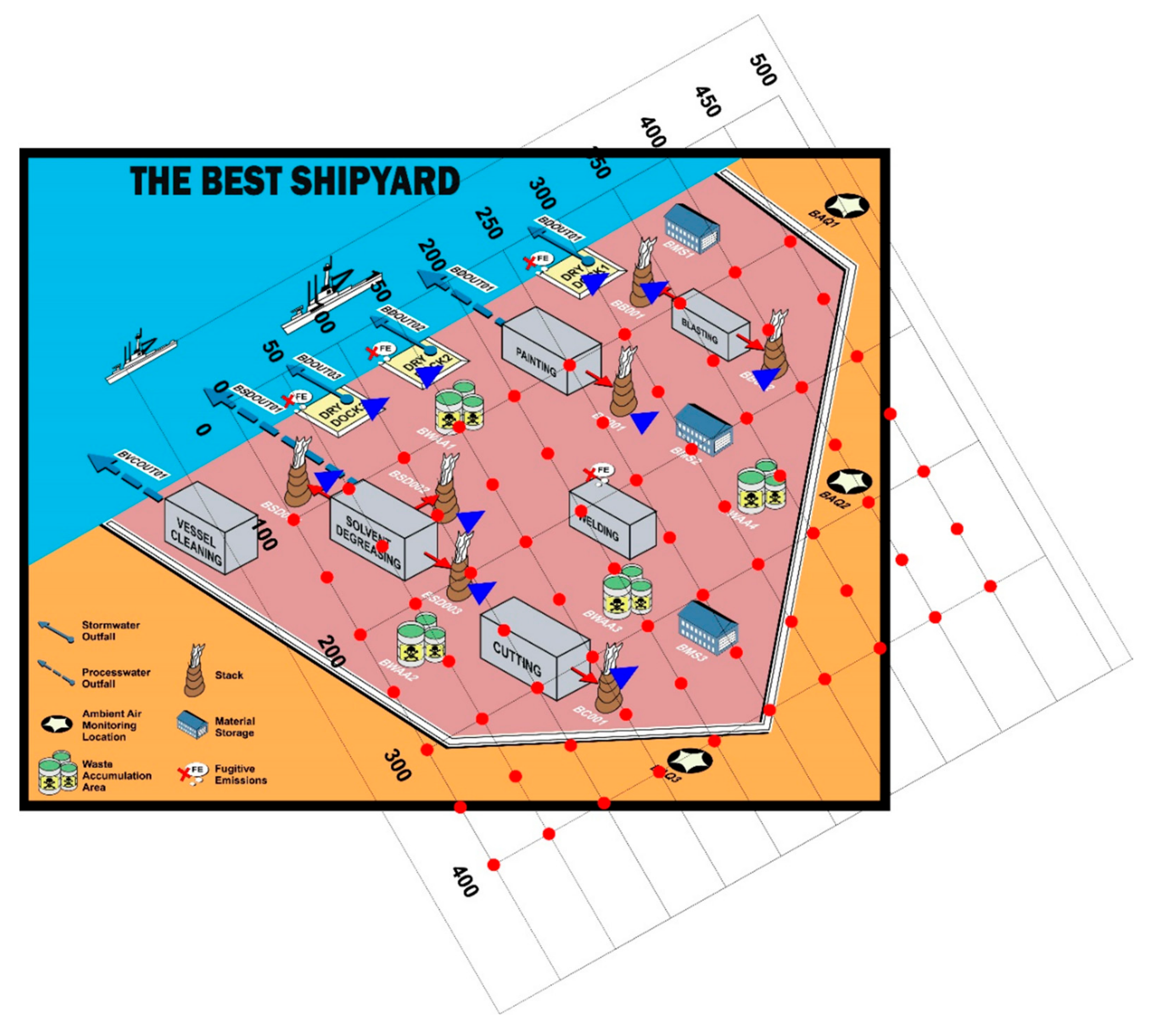
2.3. Best Shipyard Case

The Best Shipyard is a hypothetical concept created by the Maritime Environmental Resources and Information Center (MERIC) at the University of New Orleans (UNO) for educational purposes to demonstrate various shipyard processes and multimedia emissions to the students and environmental engineers/professionals, and to develop software applications. This was helpful in communicating among environmental engineering and software developers. For demonstrating the inverse dispersion model in this paper, the same hypothetical shipyard, “the Best Shipyard” was used with a layout as shown in Figure 2. This Best Shipyard has three drydocks (unknown emission rates, Q_s) and seven other stack sources (known emission rates, Q_s).

2.4. Inverse Dispersion Model for Drydocks

To evaluate the feasibility of the inverse dispersion model for drydocks, the authors in this research consider two approaches as follows (a) assuming one equivalent point source in each drydock and (b) assuming nine point sources in each drydock, considering it as an area source. The model involved in demonstrating the inverse dispersion model to drydock scenario can be described in six (6) distinct steps mentioned in the following section. For this exercise, the emission rates from all the sources in the shipyard (sources include the drydocks and other stack sources) are assumed as depicted in

Table 1. Emissions assumed for each source.

Source	x-cord (in m)	y-cord (in m)	Height (H) (in m)	Actual Emissions (in μg/s)
S1	50	100	0	7000
S2	50	150	0	7520
S3	50	300	0	8540
S4	80	40	10	7480
S5	80	340	10	9400
S6	160	120	10	12000
S7	160	280	10	1359
S8	180	380	10	16000
S9	210	100	10	18800
S10	320	160	10	1585

. For the purpose of this paper and the intended demonstration, the “actual” emissions from the ten point sources were assumed as shown in Table 1. Sources S1–S3 are the drydocks and S4–S10 are the stack sources.

A grid was laid over the Best Shipyard layout as depicted in Figure 3 with the triangular markers showing the source locations emitting air pollutants (three drydock sources and seven stack sources) and the circular markers represent the receptor locations where the concentrations are monitored. The receptor points are the points where the air pollutant concentrations can be either measured using an air quality monitor or modeled using air quality models such as atmospheric dispersion models. In this paper, modeled values at the receptors are being used but in the actual case, one must use measured/monitored air pollutant concentrations which can be achieved by either grab sampling method or real-time monitoring.

To use the Gaussian dispersion equation, the required meteorological conditions used/ assumed are as follows:

Wind Speed: 5 m/sec

Wind Direction (degree): 270 (wind blowing from West to East)

Pasquill (Atmospheric) Stability Class: C.

The six steps in discussing the model are as follows:

2.4.1. Step 1: Ten (10) Point Sources with Known Emission Rates (Q_s) to Calculate Concentrations (C_s) at Seventy (70) Receptors

The ambient concentrations resulting from known emissions from the ten sources were calculated at all 70 receptor locations. The concentrations were calculated using the Gaussian dispersion model as depicted by Equation (1). The coordinates (x and y) were computed using the source and receptor grids and are shown in Table 1 (source co-ordinates) and

Table 2. Receptor locations and concentrations as calculated in Step 1.

Receptor	x-Coord	y-coord	Concentration (µg/m3)	Receptor	x-Coord	y-Coord	Concentration (µg/m3)
R1	100	0	0	R36	250	250	0.207
R2	100	50	0	R37	250	300	1.798
R3	100	100	15.667	R38	250	350	1.256
R4	100	150	16.830	R39	250	400	0.098
R5	100	200	0	R40	250	450	0
R6	100	250	0	R41	300	0	0.253
R7	100	300	19.113	R42	300	50	0.926
R8	100	350	0	R43	300	100	3.685
R9	100	400	0	R44	300	150	1.531
R10	100	450	0	R45	300	200	0.240
R11	150	0	0	R46	300	250	0.315
R12	150	50	0.179	R47	300	300	1.457
R13	150	100	4.488	R48	300	350	1.474
R14	150	150	4.820	R49	300	400	0.987
R15	150	200	0.004	R50	300	450	0
R16	150	250	0.005	R51	350	0	0.288
R17	150	300	5.470	R52	350	50	0.876
R18	150	350	0.225	R53	350	100	4.431
R19	150	400	0	R54	350	150	1.561
R20	150	450	0	R55	350	200	0.276
R21	200	0	0.036	R56	350	250	0.376
R22	200	50	0.851	R57	350	300	1.211
R23	200	100	2.232	R58	350	350	1.736
R24	200	150	2.386	R59	350	400	1.433
R25	200	200	0.075	R60	350	450	0.012
R26	200	250	0.085	R61	400	0	0.293
R27	200	300	2.677	R62	400	50	0.990
R28	200	350	1.067	R63	400	100	3.877
R29	200	400	0.001	R64	400	150	1.672
R30	200	450	0	R65	400	200	0.315
R31	250	0	0.161	R66	400	250	0.400
R32	250	50	1.001	R67	400	300	1.026
R33	250	100	1.755	R68	400	350	1.716
R34	250	150	1.592	R69	400	400	1.419
R35	250	200	0.178	R70	400	450	0.063

(receptor co-ordinates). The drydock emission height was considered to be “0 meters” as it is believed that the most emissions from drydocks are emitted ground level. The emission height for all seven other point sources (stack sources) was considered to be “10 meters” as all the sources are connected to a stack to spew the emissions. Since there are 70 receptors and ten sources, there will be 700 (70 × 10) calculations. The MATLAB program was used to compute the pollutant concentration in ambient air at seventy (70) receptors as shown in Table 2.

The source locations (three drydocks and seven stack sources) along with receptor (70) locations as depicted using MATLAB is shown in Figure 4.

2.4.2. Step 2: Step 2: Known C_s at 70 Receptors to Calculate Three Unknown Drydock Q_s

In a real-world scenario, the concentrations are known using monitoring instruments of a different kind, depending on the type of pollutant at hand. Once these measured/monitored concentrations at various locations (receptors) are known, one has to identify the possible sources and then use the inverse dispersion model [17] to back-calculate the emission rates for these identified sources. In this paper, the calculated ambient concentrations in Step 1 will be treated as measured concentrations from this point. In Step 2, the demonstration of reverse calculation is implemented by treating the three drydock sources as unknown sources, while emissions from the stack sources are known. The concentrations from Table 2 were used to implement the inverse dispersion model to compute the emission rates from the three drydocks. Again, MATLAB was used to compute the unknown emission rates, which are shown in

Table 3. Comparison of assumed and calculated emission rates in Step 2.

Source	x-Coord (in m)	y-Coord (in m)	Height (H) (in m)	Actual Emissions (in μg/s)	Calculated Emissions (in μg/s)	Difference (in μg/s)
S1	50	100	0	7000	7000.011	−0.011
S2	50	150	0	7520	7520.015	−0.015
S3	50	300	0	8540	8539.986	0.014
S4	80	40	10	7480	7480.286	−0.286
S5	80	340	10	9400	9400.021	−0.021
S6	160	120	10	12,000	11,999.891	0.109
S7	160	280	10	1359	1358.995	0.005
S8	180	380	10	16,000	16,000.189	−0.189
S9	210	100	10	18,800	18,800.081	−0.081
S10	320	160	10	1585	1584.605	0.396

. These “computed” emission rates were compared with “actual” emission rates from Table 1 as can be seen in Table 3.

2.4.3. Step 3: Using only the Three Drydocks as the Sources with Known Emission Rates (Q_s) to Calculate C_{r, DS} at 70 Receptors

In Step 3, three drydocks with emission rates (Q_s) calculated in Step 2 were used to compute the ambient concentrations at the seventy receptors using the direct Gaussian dispersion model. The purpose was to see whether the concentrations at these 70 receptors will change with a change in the number and location of sources within the facility. These computed concentrations are depicted in

Table 4. Concentrations at all 70 receptors due to the three drydocks alone, as calculated in Step 3.

Receptor	Measured Concentration (in µg/m3)	Receptor	Measured Concentration (in µg/m3)	Receptor	Measured Concentration (in µg/m3)	Receptor	Measured Concentration (in µg/m3)
R1	0	R19	0	R37	1.565	R55	0.271
R2	0	R20	0	R38	0.201	R56	0.291
R3	15.667	R21	0	R39	0	R57	0.753
R4	16.830	R22	0.070	R40	0	R58	0.278
R5	0	R23	2.231	R41	0.004	R59	0.014
R6	0	R24	2.386	R42	0.220	R60	0
R7	19.113	R25	0.075	R43	1.090	R61	0.023
R8	0	R26	0.085	R44	1.138	R62	0.244
R9	0	R27	2.631	R45	0.240	R63	0.703
R10	0	R28	0.085	R46	0.267	R64	0.722
R11	0	R29	0	R47	1.046	R65	0.287
R12	0.004	R30	0	R48	0.264	R66	0.293
R13	4.488	R31	0	R49	0.004	R67	0.571
R14	4.820	R32	0.165	R50	0	R68	0.268
R15	0.004	R33	1.460	R51	0.012	R69	0.028
R16	0.005	R34	1.543	R52	0.241	R70	0.001
R17	5.470	R35	0.178	R53	0.862
R18	0.005	R36	0.201	R54	0.891

. The term C_{r, DS} is used to explain that the concentration is calculated for the receptor ‘r’ which is caused due to the drydock sources ‘DS.’ The results of this exercise are shown in Table 4.

2.4.4. Step 4: Seventy Receptors with Known C_{r, DS} to Compute Q_s from Nine Sources in Each of Three Drydocks (Total of 27 Sources in 3 Drydocks)

The second aspect of the research is considering each drydock as an area source. As mentioned earlier, there is no one particular emission source for a drydock. Often, repair work is carried out at many locations in the drydock, and the actual emissions take place from multiple locations within a drydock. In order to simulate this situation, a total of twenty-seven (27) point sources were considered with nine (9) sources in each of the three (3) drydocks. Figure 5 shows the distribution of sources in each drydock. The pollutant concentrations in ambient air available from Step 3 were used in combination with the inverse dispersion model to compute the unknown Q_s at twenty-seven (27) sources. Emission rates obtained from this exercise are depicted in

Table 5. Emission rates calculated in Step 4 for drydocks as an area source with nine source locations at each drydock.

Source	x-Cord (in m)	y-Cord (in m)	Calculated Emission (µg/s)	Source	x-Cord (in m)	y-Cord (in m)	Calculated Emission (µg/s)	Source	x-Cord (in m)	y-Cord (in m)	Calculated Emission (µg/s)
S11	30	110	0	S21	30	160	0	S31	30	310	0
S12	30	100	0	S22	30	150	0.158	S32	30	300	0
S13	30	90	0	S23	30	140	0	S33	30	290	0
S14	50	110	0	S24	50	160	0	S34	50	310	0.098
S15	50	100	6997.936	S25	50	150	7519.638	S35	50	300	8538.738
S16	50	90	0.204	S26	50	140	0.294	S36	50	290	0.081
S17	70	110	0	S27	70	160	0	S37	70	310	0.128
S18	70	100	0.720	S28	70	150	0.069	S38	70	300	0.429
S19	70	90	0.860	S29	70	140	0	S39	70	290	0.353
S1	TOTAL		6999.729	S2	TOTAL		7520.159	S3	TOTAL		8539.827

. The reason for this exercise is to see the difference in total emissions from each drydock between the two alternatives considered, (a) one source in each drydock and (b) nine sources in each drydock.

2.4.5. Step 5: Known Q_s at 27 Sources (3 Drydocks) to Compute C_s at 30 New Receptors

In Step 5, all 27 sources within three drydocks were considered, and ambient concentrations were computed using the Gaussian equation (MATLAB code) at 30 receptors as shown in Figure 6 (new receptor grid; different from the previous 70 receptor grid). All other parameters such as wind speed and stability class were kept the same. The purpose is to see how the concentrations at these 30 receptors will change from (a) total of 3 sources, one source in each of three drydocks to (b) total of 27 sources, nine sources in each of the three drydocks. Source-receptor geometry is illustrated in Figure 6. The computed concentrations are shown in

Table 6. Comparison of calculated ambient concentrations.

Receptor	Concentration Using Single Equivalent Source (in µg/m3)	Concentration Using Nine Sources in Each Drydock (in µg/m3)	Difference	Receptor	Concentration Using Single Equivalent Source (in µg/m3)	Concentration Using Nine Sources in Each Drydock (in µg/m3)	Difference
R1	0.915	0.915	0	R16	5.470	5.470	0
R2	2.386	2.386	0	R17	0	0	0
R3	0.003	0.003	0	R18	0.003	0.003	0
R4	2.631	2.631	0	R19	0.044	0.044	0
R5	0.724	0.724	0	R20	0.118	0.118	0
R6	1.352	1.352	0	R21	0	0	0
R7	0.055	0.055	0	R22	0.036	0.036	0
R8	1.318	1.318	0	R23	0	0	0
R9	0.520	0.520	0	R24	0.100	0.100	0
R10	0.817	0.817	0	R25	0	0	0
R11	0.177	0.177	0	R26	0.420	0.420	0
R12	0.670	0.670	0	R27	0.599	0.599	0
R13	0.761	0.761	0	R28	0.233	0.233	0
R14	4.820	4.820	0	R29	0.450	0.450	0
R15	0	0	0	R30	0.002	0.002	0

. This demonstration will help study the health impacts of the facility at various receptor locations that are of interest.

2.4.6. Step 6: Known Q_s at 3 Sources (3 Drydocks) to Compute C_s at 30 New Receptors

Now knowing the concentrations at the 30 receptors, the concept of the equivalent source is implemented using the same set of 30 receptors by combining the nine sources at each drydock to consider the drydock as a single source. Step 6 is the same as Step 5 except that only three sources (one source in each drydock) were considered for computing the concentration in ambient air at 30 newly selected receptors. The results are shown in

Table 7. Comparison of total emissions at each drydock (single equivalent source vs. nine sources in each drydock).

Drydock Number	Emissions (µg/s) (Single Equivalent Source in Each Drydock)	Emissions (µg/s) (Nine Sources in Each Drydock)	Difference
1	7000.011	6999.719	0.292
2	7520.015	7520.159	−0.145
3	8539.986	8539.827	0.159

, and the source-receptor geometry is illustrated in Figure 7. This step shows that the concept of the equivalent source can be implemented since the drydock can be considered as one source. As seen in Table 6, the error margin between the two scenarios (considering drydocks as a point source and area source) is of the magnitude 10⁻⁴.

3. Results and Discussion

Step 1 provided the results of the ambient pollutant concentration at 70 receptors, which are shown in Table 2. These ambient concentrations are computed using a simple Gaussian dispersion method described by Equation (1).

Step 2 utilizes the inverse Gaussian model proposed by Figueroa et al. (2008). This step used the ambient concentrations computed (in this case result of Step 1; field measured ambient concentrations can be used in actual applications) to compute emission rates. The results are obtained using the MATLAB code utilizing Equation (3)–(5). Here, 7 out of the ten sources considered have known emission rates since they are stack (point) sources and can be measured easily. The three drydocks are considered as unknown sources, and the emissions are computed using this inverse dispersion model described in this paper. The results of modeled Q_s for the three unknown drydock sources are shown in Table 3. From Step 2, it can be seen that the modeled results are the same as the actual emission rates (in this case, the assumed emission rates which were used in Step 1). Thus, this model proves to be very promising. Here, the actual ambient concentrations were unknown; the ambient concentrations at various receptors are calculated in Step 1. In the field, however, the concentrations will be measured using a simple hand-held instrument and carry on with Step 2 to compute the emission rate which is unknown.

Step 3 provided the results of the modeled concentrations (C_{r, DS}) at receptor “r” due to source “s” at 70 receptors from only three sources (one in each drydock). The results of this step are shown in Table 4. The concentration at each receptor is the sum of effect due to all the three sources at that receptor.

In Step 4, the authors provided the results of the emission rates (Q_s) at 27 sources (nine sources in each drydock) that were calculated using the ambient concentrations at 70 receptors. These results are presented in Table 5.

Steps 5 and 6 resulted in modeled ambient concentrations at 30 new receptors as a result of emissions from 27 sources located in three drydocks (nine sources in each drydock) and emissions from three sources located in three drydocks (one source in each drydock) which are given in Table 6.

The concept of “equivalent source” is proved in Step 4–7. The comparison shown in Table 7 proves that treating the drydock as a single point source gives comparable results with the case when the drydock is considered to have nine source locations throughout the area of the drydock as shown in Figure 5. However, caution should be used in extrapolating this approach and should be used for situations that are tested through additional validation.

The inverse dispersion model was evaluated for quantifying drydock emissions. This model is scalable and can be applied to quantify emissions from animal farms, landfills, wastewater treatment plants, forest fires and so on.

The paper mainly provided a novel method of using the Gaussian dispersion model in a reverse way to solve complex emission inventory problems that exist in the maritime industry. The authors believe that this model has significant benefits as stated below:

• The proposed model uses the proven scientific method of the Gaussian Dispersion Model, which is used by the USEPA as a regulatory model. Many countries around the World use the same model for regulatory compliance and approving air permits. The model’s limitations are well recognized, and efforts are constantly being made to improve the assumptions and algorithm. For now, the model is being used “as-is” for regulatory and litigation purposes.
• The quantification of drydock emissions is complex due to the type of operations and their variations from shipyard to shipyard. Thus, the use of emission factors available from the USEPA’s AP-42 is insufficient. There is no better method to estimate emissions from drydocks unless this area is enclosed, and source testing is conducted for each situation.
• The inverse dispersion model proposed is relatively easier to use/implement as the Gaussian Dispersion Model is already being used for regulatory purposes and is also less resource demanding.
• The lack of a rational emission quantification method will continue to result in erroneous emission estimates, thus erroneous risk assessments.
• The proposed model can be easily applied to other complex emission sources such as landfills, superfund sites, raw material yards, large mine sites, forest fires, wastewater treatment plants and many more.

4. Conclusions

This paper demonstrates the feasibility of the inverse dispersion model for quantifying emissions from drydocks that are not easily quantifiable. The results prove that this model is reliable in estimating the emission rates from sources that are not quantifiable through source monitoring methods and those that do not have reliable emission factors. The same model can be applied to quantify emission rates from landfills, animal farms, and wastewater treatment plants where the reliable emission factors are absent. Emission quantification from these sources can help various sources comply with regulations, perform impact analysis, and conduct health risk assessments in the nearby community. In most countries, it is a big challenge for any governmental agency to quantify the actual emissions from forest fires. By implementing the inverse dispersion model, it will be easier to quantify the emissions from forest fires, and this can help agencies in reporting the emissions to develop emission control strategies and health risk assessments. However, the authors caution the use of the proposed inverse dispersion model as this method relies on the applicability of the Gaussian dispersion model. Whenever and wherever the Gaussian dispersion model cannot be utilized, the proposed inverse model will have the same limitations.

References

1. Maritime Administration (MARAD). The Economic Importance of the U.S. Shipbuilding and Repairing Industry. Available online: https://www.maritime.dot.gov/sites/marad.dot.gov/files/docs/resources/3641/maradeconstudyfinalreport2015.pdf (accessed on 9 May 2019).
2. Dincer, I.; Midilli, A.; Hepbasli, A.; Karakoc, T.H. (Eds.) Global Warming Engineering Solutions Series: Green Energy and Technology; Springer: Berlin, Germany, 2010; pp. 579–590. [Google Scholar]
3. Celebi, U.B.; Ekinci, S.; Alarcin, F.; Unsalan, D. The Risk of occupational safety and health in shipbuilding industry in Turkey. In Proceedings of the 3rd International Conference on Maritime and Naval Science and Engineering, Constantza, Romania, 3–5 September 2010. [Google Scholar]
4. Papaioannou, D. Environmental implications related to the shipbuilding and ship repairing activity in Greece. J. Marit. Transp. Sci. 2003, 41, 241–252. [Google Scholar]
5. Kura, B.; Lacoste, S.; Patibanda, P. Multimedia pollutant emissions from shipbuilding facilities. In Proceedings of the United States and Japan Natural Resources (UJNR) Conference, Washington, DC, USA, 25 October–4 November 1998. [Google Scholar]
6. Celebi, U.B.; Vardar, N. Investigation of VOC Emissions from Indoor and Outdoor Painting Processes in Shipyards. Atmos. Environ. 2008, 42, 5685–5695. [Google Scholar] [CrossRef]
7. Kura, B. Multi-media pollutants in the shipbuilding industry and the importance of environmental management. In Proceedings of the 1st international symposium on Naval Architecture and Maritime, Yildiz Technical University, Istanbul, Turkey, 24–25 October 2011. [Google Scholar]
8. Kura, B.; Wisbith, A.S.; Stone, R.; Judy, T. Metal Cutting Operations: Emission Factors for Particulates, Metals and Metal Ions. In Proceedings of the Emission Inventory: Regional Strategies for the Future Proceedings, Raleigh, NC, USA, 26–28 October 1999; pp. 1–13. [Google Scholar]
9. Kura, B.; Judy, T.; Wisbith, S.A.; Stone, R. Assessment of air emissions from shipyard cutting processes. In Proceedings of the United States Japan Natural Resources (UJNR) Conference, Tokyo, Japan, 17–18 May 2000; pp. 1–18. [Google Scholar]
10. Celebi, U.B.; Mert, T.; Bilgili, L.; Senoz, K.M.; Ekinci, S. Characterization of sub-micrometer fume particles in MMA welding of shipbuilding steel with different types of electrodes. Fresenius Environ. Bull. 2017, 26, 140–145. [Google Scholar]
11. Mert, T.; Ekinci, S. Fume formation rate analysis of shipbuilding steel with SMAW using Taguchi design and ANOVA. Acta Phys. Pol. A. 2017, 13, 495–499. [Google Scholar] [CrossRef]
12. Kura, B.; Kambham, K.; Sangameswaran, S.; Potana, S. Atmospheric particulate emissions from dry abrasive blasting using coal slag. J. Air Waste Manag. Assoc. 2006, 56, 1205–1215. [Google Scholar] [CrossRef] [PubMed]
13. U.S. Environmental Protection Agency. Office of Compliance Sector Notebook Project: Profile of the Shipbuilding and Repair Industry; EPA/310-R-97-008; U.S. Environmental Protection Agency: Washington, DC, USA, 1997.
14. U.S. Environmental Protection Agency. Sector Performance Report. Shipbuilding & Ship Repair. Available online: https://archive.epa.gov/sectors/web/pdf/shipbuilding.pdf (accessed on 9 May 2019).
15. U.S. Environmental Protection Agency. Technology Transfer Network Air Toxics Web Site. Emissions Factors & AP 42, Compilation of Air Pollutant Emission Factors. Available online: http://www.epa.gov/ttnchie1/ap42/ (accessed on 9 May 2019).
16. Flesch, T.K.; Wilson, J.D.; Harper, L.A.; Crenna, B.P. Estimating gas emissions from a farm with an inverse-dispersion technique. Atmos. Environ. 2005, 39, 4863–4874. [Google Scholar] [CrossRef]
17. Figueroa, V.K.; Cooper, C.D.; Mackie, K.R. Estimating landfill greenhouse gas emissions from measured ambient methane concentrations and dispersion modeling. In Proceedings of the 101st Air and Waste Management Association Annual Conference and Exhibition, Portland, OR, USA, 24–27 June 2008. [Google Scholar]
18. Faulkner, W.B.; Goodrich, L.B.; Botlaguduru, V.S.V.; Capareda, S.C.; Parnell, C.B. Particulate matter emission factors for almond harvest as a function of harvester speed. J. Air Waste Manag. Assoc. 2009, 59, 943–949. [Google Scholar] [CrossRef] [PubMed]
19. Figueroa, V.K.; Mackie, K.R.; Guarriello, N.; Cooper, C.D. A robust method for estimating landfill methane emissions. J. Air Waste Manag. Assoc. 2009, 59, 925–935. [Google Scholar] [CrossRef] [PubMed]
20. Flesch, T.K.; Harper, L.A.; Desjardins, R.L.; Gao, Z.; Crenna, B.P. Multi-source emission determination using an inverse-dispersion technique. Bound. Layer Meteorol. 2009, 132, 11–30. [Google Scholar] [CrossRef]
21. Lushi, E.; Stockie, J.M. An inverse Gaussian plume approach for estimating atmospheric pollutant emissions from multiple point sources. Atmos. Environ. 2010, 44, 1097–1107. [Google Scholar] [CrossRef] [Green Version]
22. Schauberger, G.; Piringer, M.; Knauder, W.; Petz, E. Odour emissions from a waste treatment plant using an inverse dispersion technique. Atmos. Environ. 2011, 45, 1639–1647. [Google Scholar] [CrossRef]
23. Bonifacio, H.F.; Maghirang, R.G.; Auvermann, B.W.; Razote, E.B.; Murphy, J.P.; Harner, J.P., III. Particulate matter emission rates from beef cattle feedlots in Kansas-reverse dispersion modeling. J. Air Waste Manag. Assoc. 2012, 62, 350–361. [Google Scholar] [CrossRef] [PubMed]
24. U.S. Environmental Protection Agency. United States Environmental Protection Agency, “User’s Guide for the Industrial Source Complex (ISC3) Dispersion Models. Volume II—Description of Model Algorithms”; U.S. Environmental Protection Agency: Washington, DC, USA, 1995.
25. Perry, S.G.; Cimorelli, A.J.; Lee, R.F.; Paine, R.J.; Venkatram, A.; Weil, J.C.; Wilson, R.B. AERMOD: A dispersion model for industrial source applications. In Proceedings of the 87th Annual Meeting Air and Waste Management Association, Pittsburgh, PA, USA, 19–24 June 1994; p. 16. [Google Scholar]
26. Cooper, C.D.; Alley, F.C. Air Pollution Control, A Design Approach, 4th ed.; Waveland Press: Long Grove, IL, USA, 2011. [Google Scholar]
Figure 1. Gaussian dispersion model [26].
Atmosphere 10 00328 g001
Figure 2. The best shipyard–A hypothetical layout for demonstration.
Atmosphere 10 00328 g002
Figure 3. The Best Shipyard case with the grid superimposed in MATLAB. The triangles and circles depict sources and receptors respectively.
Atmosphere 10 00328 g003
Figure 4. Grid showing ten Sources and 70 receptors as generated in MATLAB.
Atmosphere 10 00328 g004
Figure 5. (a) One source in each of the three drydocks vs. (b) nine sources in each of the three drydocks.
Atmosphere 10 00328 g005
Figure 6. Source-receptor geometry for nine sources at each drydock and a total of 27 sources at the facility.
Atmosphere 10 00328 g006
Figure 7. New source-receptor grid with the three drydocks.
Atmosphere 10 00328 g007