Southern Hemisphere Sensitivity to ENSO Patterns and Intensities: Impacts over Subtropical South America

Abstract

El Niño flavors influence Subtropical South American (SSA) rainfall through the generation of one or two quasi-stationary Rossby waves. However, it is not yet clear whether the induced wave trains depend on the El Niño pattern and/or its intensity. To investigate this, we performed different sensitivity experiments using an Atmospheric General Circulation Model (AGCM) which was forced considering separately the Canonical and the El Niño Modoki patterns with sea surface temperature (SST) maximum anomalies of 1 and 3 °C. Experiments with 3 °C show that the Canonical El Niño induces two Rossby wave trains, a large one emanating from the western subtropical Pacific and a shorter one initiated over the central-eastern subtropical South Pacific. Only the shorter wave plays a role in generating negative outgoing longwave radiation (OLR) anomalies over SSA. On the other hand, 3 °C El Niño Modoki experiments show the generation of a large Rossby wave train that emanates from the subtropical western south Pacific and reaches South America (SA), promoting the development of negative OLR anomalies over SSA. Experiments with 1 °C show no impacts on OLR anomalies over SSA associated with El Niño Modoki. However, for the Canonical El Niño case there is a statistically significant reduction of the OLR anomalies over SSA related to the intensification of the upper level jet stream over the region. Finally, our model results suggest that SSA is more sensitive to the Canonical El Niño, although this result may be model dependent.

1. Introduction

El Niño Southern Oscillation (ENSO) is the main interannual variability phenomenon in the climate system that strongly impacts climate in many regions worldwide [1,2,3,4,5]. Until approximately the 1990s, most of El Niño events were characterized by maximum tropical sea surface temperature (SST) anomalies located over the eastern equatorial Pacific. For this reason, such Canonical El Niño events are also referred to as Eastern Pacific El Niño (EP, [6]). However, other studies have shown that El Niño events with maximum tropical SST variability located over the central equatorial Pacific started to be more frequent since the 1990s [7]. These events were baptized as “dateline El Niño” by Larkin and Harrison [8], and as El Niño Modoki by Ashok et al. [9], although nowadays most of the studies refer to this type of El Niño as Central Pacific El Niño [10,11].

Given that the position of the maximum SST anomalies is directly related to the diabatic heating released over the equatorial Pacific in upper levels, different SST anomaly patterns can induce different upper level divergent circulation anomalies that, in turn, can generate changes in the tropical-extratropical teleconnection patterns [12,13,14,15]. As consequence of this, in recent years there has been a flurry of activity to determine the teleconnection patterns associated with these two different types of El Niño.

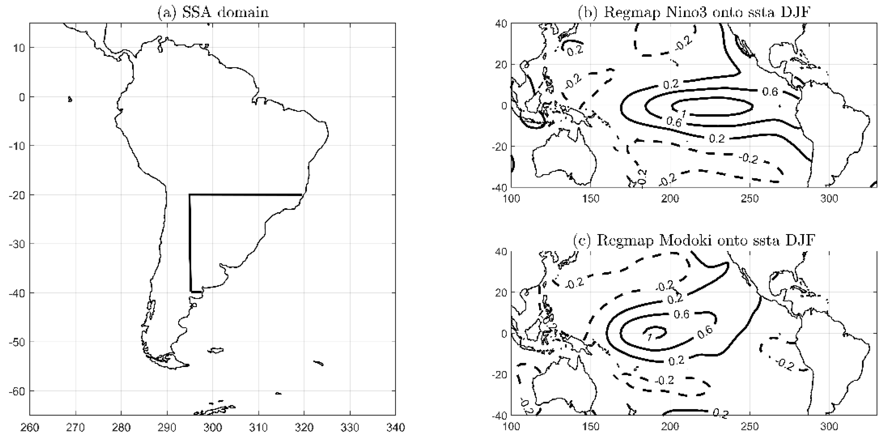
One of the regions most affected by El Niño is Subtropical South America (SSA, see Figure 1a), a region located east of the Andes mountains between 20° S and 40° S and with watershed in the tropical Atlantic (Figure 1a; e.g., [10,11,15,16,17]). In this study, we focus on the impacts of the positive phase of these two different El Niño patterns on SSA rainfall during the austral summer season, here defined as December-January-February (DJF).

Focusing on Canonical El Niño events, many previous studies have shown that this pattern increases precipitation over SSA through (1) an increase in the advection of cyclonic vorticity in upper levels that favors the development of baroclinicity, and/or (2) the intensification of the moisture transport from the tropics toward SSA that enhances the availability of moisture for precipitation over the region [12,15,16,18]. These two factors, moisture availability at lower levels and dynamic lift, are the ingredients needed to develop rainfall anomalies. Andreoli et al. [10] also show positive rainfall anomalies over SSA associated with the Canonical El Niño event, but the signal is only statistically significant over a small region within SSA that covers part of the Argentinian’s provinces of Mendoza and Córdoba. This discrepancy with the rest of the studies could be related to the period considered by Andreoli et al. [10]: they focused on precipitation anomalies over the period 1901–2010 and it is known that the quality of the reanalysis before 1979 in the Southern Hemisphere (SH) is poor because of the lack of observed data.

Focusing on El Niño Modoki events, their influence on SSA rainfall anomalies is not yet clear. Some studies have shown a negative and statistically significant precipitation signal over SSA during an El Niño Modoki (see Figure 4 from Weng et al. [13]). Results from Tedeschi et al. [15] and Brito [19] also point in this direction although the negative precipitation signal over SSA is not found to be statistically significant. However, there are other studies suggesting the opposite, an increase of SSA precipitation during El Niño Modoki [18]. Andreoli et al. [10] also show positive rainfall anomalies over SSA, but the signal is statistically significant only in some small regions. Differences among studies can arise from the dataset employed, the period considered and the methodology used to define the El Niño Modoki index.

Studies have also shown that the upper level circulation anomalies associated with El Niño Modoki present a different spatial structure from those related to Canonical El Niño, with the former not showing a clear Rossby wave pattern propagating over the extratropical latitudes in the SH during the austral summer season [10,11,13,14]. Weng et al., [13] is an exception, as their results (see their Figure 8) suggest that, associated with El Niño Modoki, there could be a weak Rossby wave pattern that emanates from the western Subtropical Pacific and propagates to the east, but it does not reach the South Atlantic Ocean. Some differences may result from the fact that Weng et al. [13] analyze the January-February-March season, while the other previously mentioned studies focus on DJF. Nevertheless, all studies agree in the weaker intensity of the upper level circulation anomalies associated with El Niño Modoki in comparison with those related to the Canonical El Niño. However, the absence of a clear Rossby wave pattern associated with El Niño Modoki could be related to: (1) the smaller intensity of SST anomalies that characterize such events in comparison with the Canonical ones, and (2) a possible lower sensitivity of the atmosphere to the pattern of SST anomalies.

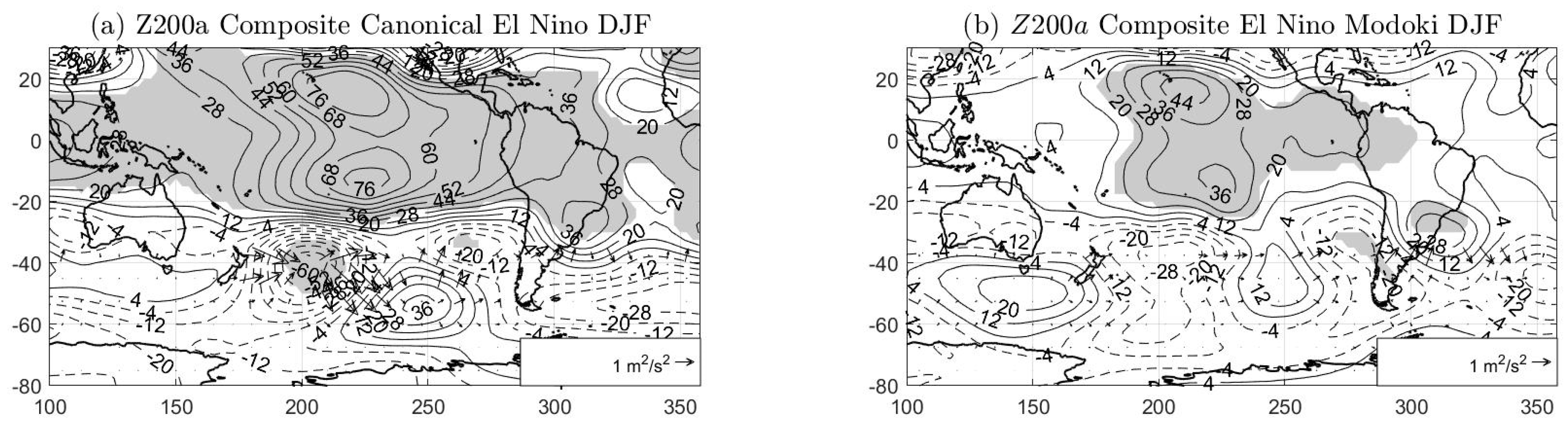
It is also worth mentioning that although there is, overall, agreement in the literature about the induced rainfall anomalies over SSA in the case of the Canonical El Niño events, the upper level circulation pattern observed over the SH is not exactly the same in all of them. For example, results from Sun et al. [14], based on a partial correlation analysis, suggest that the upper level circulation anomalies related to Canonical El Niño events are characterized by a large Rossby wave train that emanates from eastern New Zealand (NZ) and propagates southeastward in an arc-like trajectory reaching the South Atlantic ocean (see their Figure 4a). This large Rossby wave train structure can also be discerned in Tedeschi et al. [15] (see their Figure 10c). Additionally, a shorter Rossby wave seems to be emanating from the central-east subtropical south Pacific, although it does not seem to present an eastward propagation (Figure 4a from Sun et al. [14]). On the other hand, Figure 10c from Tedeschi et al. [15] suggests the existence of a short wave emanating from (30° S, 260° E) which could be propagating toward the northeast, generating an anomalous anticyclonic circulation over the northeastern SSA. The main difference between both studies is the strength of the events analyzed. While Sun et al. [14] evaluate all the Canonical El Niño events (stronger and weaker), Tedeschi et al. [15] focus mainly on the stronger ones. This could suggest that the shorter Rossby wave train may effectively propagate eastwards only in the strongest Canonical El Niño events.

An understanding of the conditions for the generation of the shorter Rossby wave is important for SSA rainfall, because this wave train has been shown to play a major role in increasing precipitation in the region [17]. Barreiro [17] explored the interannual variability of the extratropical transient activity in the SH and its influence on the austral summer precipitation over Uruguay. The author found that El Niño influences southern Uruguay when there is a southward displacement of the transient activity, which occurs when the two stationary waves are forced from the equatorial Pacific. The two stationary Rossby wave trains result in a large one that emanates from the central subtropical Pacific and propagates toward the south Atlantic Ocean in an arc-like trajectory, and a shorter one that emanates from the subtropical eastern south Pacific and propagates northeastward. Only when this short wave is strong, surface northerlies reach southern Uruguay and favor the increase of precipitation in the region [17]. This seems to occur when the SST anomalies associated with El Niño are located in the region of Niño3.4, an index that cannot separate between Central and Eastern El Niño events (see their Figures 11a and 9d).

Finally, Weng et al. [13] show the existence of two Rossby wave trains associated with Canonical El Niño, one of them emanating from the subtropical central Pacific and the other from the western South Pacific (their Figure 8a). Differently to what was reported by Sun et al. [13] and Tedeschi et al. [15], both of these wave trains propagate southeastward converging around (60° S, 120° E), where they propagate eastward. Such contrasting results might be a consequence of considering January-February-March season, instead of DJF.

Therefore, most studies show one or two Rossby wave trains as a response to Canonical El Niño events, but the presence or not of the shorter wave is not clear yet. In the case of El Niño Modoki, most studies do not show a clear wave train. This weaker response could be related to the fact that the SST anomalies associated with El Niño Modoki events are weaker than in the case of Canonical El Niño, or to the SST pattern itself.

The aim of this study was to understand whether the different response over SSA to El Niño depends on its intensity or/and on its spatial pattern. Special attention was paid to the number and characteristics of the quasi-stationary Rossby wave trains developed in response to the El Niño over the SH. Our approach is based on performing sensitivity experiments with an Atmosphere General Circulation Model (AGCM) in order to analyze the SH sensitivity to different El Niño patterns and intensities.

The rest of the paper is structured as follows: In Section 2, we explain the data and methodology used. Then, in Section 3, we focus on the analysis of the SH circulation response to the Canonical El Niño and El Niño Modoki patterns using reanalysis data. After that, in Section 4, we investigate the SH circulation sensitivity to different ENSO’s patterns and intensities considering idealized sensitivity experiments. Finally, in Section 5 we present the main conclusions of the work.

2. Data and Methods

To analyze the SH circulation response to different ENSO patterns and intensities and their impacts over SSA (see Figure 1a), we focused on the austral summer season during the period 1979–2016 and considered both reanalysis data and the output from an AGCM. Reanalysis data was first considered to analyze the atmospheric response to different ENSO patterns and then to check whether the model could reproduce the atmospheric response to both El Niño patterns. The AGCM was used to perform sensitivity experiments and test the changes in the atmospheric response to different ENSO patterns and intensities.

The analysis of the observed data was carried out considering monthly values of (1) sea surface temperature (SST) from ERSSTv4 [20], (2) interpolated outgoing longwave radiation (OLR) at the top of the atmosphere from National Oceanic and Atmospheric Administration (NOAA) [21], (3) horizontal wind at 850 hPa (v850) and geopotential height at 200 hPa (z200) from National Center of Environmental Prediction / Department of Energy (NCEP/DOE Reanalysis 2) [22]. We first computed the anomaly values of OLR, z200 and v850 fields by removing the seasonal cycle during the analyzed period (1979–2016). They were referred to as OLRa, z200a and v850a, respectively. Then, to discriminate between the two types of El Niño, Canonical and Modoki, we used the Niño3 and the El Niño Modoki (MI) indices, respectively. The Niño3 index was defined as the DJF SST anomaly averaged over the region (150° W-90° W, 5° S-5° N), while the MI index was calculated considering the improved definition given by Li et al. [23]: MI = 3·[SSTa]_A − 2·[SSTa]_B − [SSTa]_C, where [SSTa]_X refers to the average of the DJF SST anomalies over the box X, where X can be A = [165° E-140° W, 10° S-10° N], B = [110° W-70° W, 15° S-5° N] and C = [125° E-145° E, 10 °S-20° N].

In order to analyze the atmospheric response using reanalysis data, correlation maps between these two ENSO indices (Niño3/Modoki index) and the OLRa, z200a and v850a fields were computed. Finally, in order to make more comparable results from reanalysis and model simulations, we also computed the composite map of z200 anomalies associated with Canonical El Niño and El Niño Modoki. They were obtained considering the Canonical and Modoki El Niño events separately. The El Niño3 (El Niño Modoki) years were selected as those years when the index was greater than 0.7σ_N3 (0.7σ_Mo), where σ_N3 (σ_Mo) represents the standard deviation of El Niño3 (El Niño Modoki) index over the period 1979–2016. Finally, given that the definition of El Niño Modoki index consists in the subtraction of different SSTa averaged over different boxes (A, B and C), large anomalies over the regions B and C could indicate an El Niño year even when the SSTa over the region A were small. Moreover, an El Niño could be selected as La Niña. Therefore, an additional constraint was included to define El Niño Modoki years: region A had to present strong SSTa. Thus, El Niño Modoki years were those when MI was higher than 0.7σ_Mo and [SSTa]_A was greater than 0.7σ_[SSTa]A, where σ_[SSTa]A represents the standard deviation of the SST anomalies over the region A. This methodology was also employed by Tedeschi et al. [15].

Table 1. El Niño3 and El Niño Modoki years over the period (1979–2016) following the same criterion as in Tedeschi et al., [15] (see text for details). Gray shaded boxes were common years. The year 1982/1983 means December 1982 and January-February 1983.

Niño3	1982/1983	1986/1987	1991/1992	1997/1998	2006/2007	2009/2010	2015/2016
Niño Modoki	1991/1992	1994/1995	2002/2003	2004/2005	2009/2010	2014/2015	---

shows the El Niño3 and El Niño Modoki years. The years marked in gray were common, that is, they satisfied the criterion for strong Canonical or Modoki El Niño. These cases were classified as one or the other attending to the spatial distribution of the SST anomalies, in such a way that those common years with the stronger SST anomalies located in the region A were classified as El Niño Modoki years, and those with the maximum SST anomalies over the eastern equatorial Pacific as El Niño3 years. The final selection of years for the composite analysis is shown in

Table 2. El Niño3 and El Niño Modoki years over the period (1979–2016) used to compute the composite maps.

Niño3	1982/1983	1986/1987	1997/1998	2006/2007	2015/2016	---
Niño Modoki	1991/1992	1994/1995	2002/2003	2004/2005	2009/2010	2014/2015

. The neutral years were selected as those when both Niño3 and Modoki indices were lower than 0.7 times the respective standard deviation.

Table 3. Neutral years over the period (1979–2016) used to compute the composite maps.

Neutral Years
1979/1980	1980/1981	1981/1982
1983/1984	1987/1988	1989/1990
1992/1993	1993/1994	2001/2002
2003/2004	2012/2013	2013/2014

lists the years selected as neutral in the period (1979–2016).

The sensitivity of SH circulation to different ENSO patterns and intensities was addressed by performing idealized sensitivity experiments with the AGCM developed by the International Center for Theoretical Physics (ICTP-AGCM, hereafter Speedy; [24,25]). Speedy is a so-called intermediate complexity AGCM based on a spectral dynamical core. It is a sigma-coordinate, hydrostatic, spectral-transform model in the vorticity-divergence form with a semi-implicit treatment of gravity waves. Its prognostic variables are divergence, vorticity, absolute temperature and the surface pressure logarithm. The time stepping uses a leapfrog scheme (see Reference [24] and references therein). The horizontal resolution corresponds to a triangular spectral truncation at total wavenumber 30 (T30), with a standard Gaussian grid of 96 by 48 points. This model has been previously used to study climate variability over South America many times, showing its suitability for these kind of studies [26,27].

Given that this study focused on the impacts of the positive phase of these ENSO patterns, we constructed two ensembles of experiments using as boundary conditions the SST anomaly patterns of Canonical El Niño and El Niño Modoki, separately. The boundary conditions were constructed by adding the monthly climatological SST over the period 1979–2016 to the regression of monthly observed SST anomalies onto the DJF Niño3 and MI indices. Experiments started on 1st October and finished on 31st March. Additionally, to study the atmospheric sensitivity to different El Niño intensities, all regressions maps were multiplied by a factor in order to make the maximum SSTa intensity equal to 1 and 3 °C, maintaining the same spatial structure of SST anomalies. We selected 1 °C because it is the standard deviation of the Niño3 region, and 3 °C because this intensity represents a strong Canonical El Niño event. To facilitate the comparison between both El Niño types, intensities of 1 and 3 °C were also considered for El Niño Modoki pattern. Therefore, we set up four experiments (summarized in Table 1): Canonical El Niño 1 °C (Canonical_1C), Canonical El Niño 3 °C (Canonical_3C), El Niño Modoki 1 °C (Modoki_1C) and El Niño Modoki 3 °C (Modoki_3C). Figure 1b,c show the average DJF SST anomaly patterns associated with Canonical El Niño and El Niño Modoki with which the model was forced (see

Table 4. Summary of the experiments performed with the Atmosphere General Circulation Model (AGCM).

SSTa Pattern/Intensity	Canonical El Niño	El Niño Modoki	Climatology
1 °C	Canonical_1C (22 simulations)	Modoki_1C (22 simulations)	CONTROL run (22 simulations considering only climatological SST from 1979 to 2016)
3 °C	Canonical_3C (22 simulations)	Modoki_3C (22 simulations)

).

Each experiment consisted of 22 simulations, all of them initialized with different atmospheric initial conditions but all having the same SST as boundary conditions. The model started from rest and it was initialized by introducing a random diabatic forcing during the first days of the simulations. The spatial distribution of the diabatic forcing changed in consecutive simulations, generating different initial conditions. Additionally, a 22-member CONTROL experiment was constructed, with climatological SST as boundary conditions. Although all simulations were started on 1st October and finished on 31st March, only the season DJF was considered in this study.

To calculate the model forced response associated with each type of El Niño, we considered the ensemble mean of each experiment, which filtered out the internal atmospheric variability [28,29,30], and subtracted the CONTROL mean conditions.

Finally, in this study we have used the El Niño patterns obtained from the ERSSTv4 dataset to force the model. The patterns that can be obtained using ERSSTv5 present large similarities with those one from ERSSTv4 (not shown) and the small differences were negligible for speedy resolution (which was 3.7°).

On the other hand, to analyze wave propagation, we also computed the horizontal components of the quasi-stationary wave propagation (F_s) considering the definition given by Plumb [31]:

$$F_s=pcos\left(\varphi \right)\left(v^{\prime 2}-\frac{1}{2a}\Omega sin\left(2\varphi \right)·\frac{\partial v^{\prime }{z}^{\prime }}{\partial \lambda },-u^{\prime }{v}^{\prime }+\frac{1}{2a\Omega sin\left(2\varphi \right)}·\frac{\partial u^{\prime }{z}^{\prime }}{\partial \lambda }\right)$$

(1)

where $\varphi$ is the latitude, $a$ is the Earth’s radius, $\Omega$ is the angular rotation rate of the Earth, $u^{\prime }$ and $v^{\prime }$ are the eddy horizontal geostrophic wind components at 200 hPa averaged over DJF, and $z^{\prime }$ is the eddy geopotential height at 200 hPa averaged over DJF. For steady conservative waves, this field is nondivergent and, for slowly varying almost plane waves it is parallel to the group velocity [29]. Therefore, this measure helped us to better interpret the Rossby waves propagation associated with the El Niño phenomenon in the SH.

Finally, for a better understanding of the origin of these Rossby waves, the Rossby Wave Sources (RWS) were also computed in each experiment following the definition:

RWS = − ∇.(V_χ ξ)

(2)

where V_χ represents the divergent wind component and ξ = (f + ζ) the absolute vorticity. Equation (2) can be also expressed as:

RWS = −ξ ∇.V_χ − V_χ·∇ξ

(3)

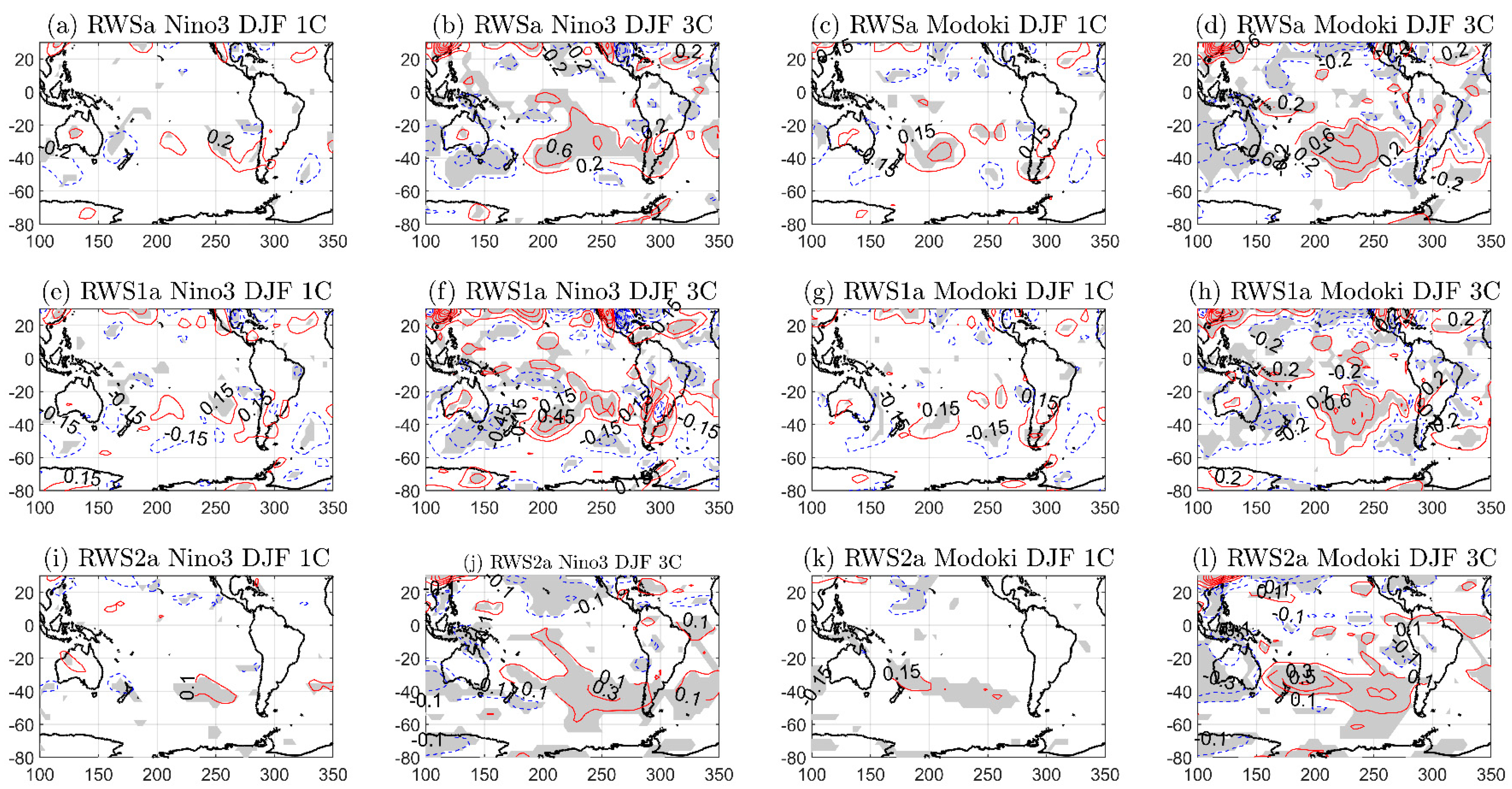
where the first term, RWS1 = −ξ ∇.V_χ, is known as the vortex stretching and the second one, RWS2 = −V_χ ·∇ξ, represents the advection of absolute vorticity by the divergent wind component. The relative vorticity ζ was computed using the rotational daily horizontal winds. In the SH, negative (positive) RWS are associated with a cyclonic (anticyclonic) circulation.

3. Results from Reanalysis

3.1. Canonical El Niño

For the Canonical El Niño, OLR correlation maps were characterized by strong negative correlation values over SSA (Figure 2a), suggesting an increase of precipitation when the positive phase of the Canonical El Niño takes place. Figure 2b shows that the upper level circulation anomaly pattern was characterized by an anomalous cyclonic circulation around (35° S, 265° E) and an anomalous anticyclonic circulation over northeastern SSA around (28° S, 315° E). The combination of these two circulation anomalies induced a strong geopotential height gradient over SSA and favored advection of cyclonic vorticity over there (in agreement with References [2,17,32]). Comparing with Figure 3a, where the composite map of the Canonical El Niño events was plotted, it was possible to see that the distribution of the extratropical z200 anomalies was similar with both metrics. This result suggested that the atmospheric response associated with Canonical El Niño is highly linear. Figure 3a also shows the F_s field, which suggested the presence of a large Rossby wave propagating from the central-western subtropical Pacific, around (40° S, 200° E), toward the southeast. However, z200 anomalies were not significant at extratropical latitudes. Additionally, it was possible to see a short Rossby wave train excited in the central-tropical Pacific, around (35° S, 270° E), that propagated eastward inducing an anomalous anticyclonic circulation over northeastern SSA around (25° S, 310° E). As in the correlation map (Figure 2b), these circulation anomalies induced a strong geopotential height gradient over SSA and favored the advection of cyclonic vorticity (Figure 3a), in agreement with References [2,17,32].

The anomalous circulation at 850 hPa revealed an equivalent barotropic behavior of the atmosphere at middle latitudes (see Figure 2b and compare with Figure 2c). Focusing on Figure 2, it was possible to see that over SSA there was a strong increase of the northerlies that brought warm and humid air from the tropics toward SSA [12,16,33]. These increased northerlies were related to the strong z200 gradient over SSA developed by the cyclone-anticyclone system located aloft and associated with the short Rossby wave. The combination of the increased cyclonic vorticity advection over SSA together with the lower level increased of moisture advection toward SSA, favored the development of cloudiness, reduced the OLR anomalies and increased precipitation over the area of study.

3.2. El Niño Modoki

Similarly to the Canonical case, negative OLR correlation values could be observed over SSA in response to El Niño Modoki although in this case the signal was not statistically significant (compare Figure 2a,c). In the upper level, the z200 correlation map did not show any structure of a clear Rossby wave propagation from the subtropical western South Pacific (see Figure 2e) and neither was there statistically significant changes in the circulation at lower levels over South America (see Figure 2f). Figure 3b shows the composite map for the case of El Niño Modoki, which showed some dissimilarities with the regression map (Figure 2e), especially over the South Pacific. However, both maps agreed over southern South America, where a wave propagation from the anomalous cyclonic circulation located eastward of South America to the anticyclonic circulation which developed around southeast Brazil could be found. Dissimilarities between the z200 correlation map and z200 composite maps were higher for El Niño Modoki than for the Canonical one (compare Figure 2b with Figure 3a, and Figure 2e with Figure 3b), which could have been related to the weaker intensity of SST anomalies associated to El Niño Modoki events (not shown).

Finally, taking into account the values of the correlation coefficients shown in Figure 2b,e, it was possible to see that the sensitivity of the atmosphere to Canonical El Niño index was much larger than in the case of El Niño Modoki. Thus, the OLRa signal associated with the Canonical El Niño was more robust than in the case of El Niño Modoki index, which was probably the reason for the controversy existing in the literature about the influence of El Niño Modoki on SSA rainfall.

4. Model Results

4.1. Canonical El Niño

Figure 4 shows the model’s response to Canonical El Niño. The first row refers to Canonical_1C experiments and the second one to the Canonical_3C experiments.

Focusing on the Canonical_1C experiment, it was possible to see negative and statistically significant OLR anomalies over the latitudinal band (28° S-35° S), suggesting an increase of precipitation over this region when a Canonical El Niño event takes place.

In upper levels, Figure 4b shows the generation of a large Rossby wave train that emanated from the subtropical western Pacific, around (40° S, 180° E). The F_s field suggested a wave propagation southeastward, although like in the reanalysis, there was no statistically significant z200 anomalies at higher latitudes over the South Pacific (compare Figure 3a and Figure 4b). At lower levels, Figure 4c shows a clear barotropic behavior of the midlatitudes atmosphere, although there were no statistically significant anomalies over SA (see Figure 4c). In this case, the strong z200a gradient developed over SSA increased the intensity of the upper level jet stream and favored the development of negative OLR anomalies over SSA (see Figure 4b,c).

When the intensity of the SST forcing was increased, the atmospheric response was stronger and significant negative OLR values were larger and covered all SSA (Figure 4d). The increased intensity in OLRa was related to anomalous changes in the upper and lower level circulations. In upper levels, the z200a pattern showed an anomalous cyclonic circulation around (35° S, 285° E) that significantly increased the advection of cyclonic vorticity over SSA (Figure 4e). This cyclonic circulation could be part of a short Rossby wave that emanated from the eastern subtropical Pacific and did not seem to cross SA. At lower levels there was a strong increase of the northerlies bringing moisture toward SSA (Figure 4f).

Additionally, the z200a pattern (Figure 4e) showed a larger Rossby wave train that emanated from the subtropical western South Pacific, around (40° S, 185° E), and propagated southeastward.

The comparison of both experiments suggested that the atmospheric response to the Canonical El Niño was highly linear. The spatial structure of the z200a pattern over the South Pacific was similar in both cases, although for Canonical_1C the anomalies were not significant. Some differences could be observed in the position of the circulation anomalies in the eastern South Pacific and over the South Atlantic Ocean (compare Figure 4b,e).

Comparing the model results with reanalysis, dissimilarities were higher in the South Atlantic Ocean, where the model did not reproduce the anticyclonic circulation over the eastern SSA associated with the shorter Rossby wave (see Figure 2b or Figure 3a and compared with Figure 4e). Additionally, the higher resemblance of the Canonical_3D OLR and z200a anomalous patterns to the ones obtained from reanalysis suggested that SPEEDY presented less sensitivity to SST anomalies than the real atmosphere, which was probably a consequence of its simplified convective parameterizations.

4.2. El Niño Modoki

Figure 5a shows that an El Niño Modoki_1C did not induce a statistically significant impact on OLR anomalies over SSA. The z200a pattern did not show any statistically significant Rossby wave as a response to El Niño Modoki_1C (see Figure 5b).

The development of negative OLR anomalies over the northern SSA within the latitudinal band (20° S-25° S) took place when increasing the intensity of the SST anomalies up to 3 °C (see Figure 5d). These anomalies were mainly related to an increase of the upper level cyclonic vorticity advection which was associated with the anomalous cyclonic circulation developed around (20° S, 270° E). The z200a pattern showed over the tropics a baroclinic Gill-Matsuno-type quadrupole structure as a response to El Niño Modoki (in agreement with Figure 10 from Taschetto et al. [34]). At extratropical latitudes, there was a large Rossby wave train generated over the subtropical western South Pacific, around (40° S, 200° E), that propagated eastward (Figure 4e) and, at the longitude of 250° E, one part of the wave activity seemed to be deflected northward and the another portion continues propagating toward the South Atlantic and northeastern SSA. Therefore, the anomalous cyclonic circulation developed around (20° S, 270° E) seemed to arise from the contribution of two factors: (1) the tropical baroclinic Gill-Matsuno quadrupole response of the atmosphere to El Niño Modoki and (2) the extratropical wave propagation (see Figure 5e). Additionally, it was possible to see a weak wave activity propagation from the anomalous cyclonic circulation located over (20° S, 270° E) to the anomalous anticyclonic circulation generated over the northeastern SSA.

At lower levels, the circulation anomaly pattern presented a barotropic behavior to the south of 30° S (compare Figure 5e,f).

From these results, one can conclude that the impact of El Niño Modoki on SSA depended on the intensity of the SST anomaly pattern, in such a way that only strong El Niño Modoki events could produce OLR anomalies over the northern SSA. The comparison of the z200a patterns from both El Niño Modoki experiments suggested that the response of the atmosphere to changes in the SST anomalies intensity in this case was more non lineal than in the case of El Canonical El Niño (compare Figure 5b,e). In addition, similarities with the observed response to El Niño Modoki were higher for the case of El Niño Modoki_3C than for the Modoki_1C experiment (Figure 3b and Figure 5b,e).

4.3. Discussion of the Model’s Results

The influence of different El Niño patterns and intensities on the SH circulation anomalies and its impacts over SSA has been analyzed by means of sensitivity experiments. As expected, we saw that stronger SST anomalies over the equatorial Pacific were related to larger circulation anomalies and more intense OLR anomalies over SSA. Additionally, the spatial distribution of the OLR anomalies changed not only with the El Niño pattern considered, but also with its intensity.

Results from Canonical El Niño experiments suggested that this type of El Niño pattern induces two statistically significant Rossby wave trains in upper levels for the case of a strong SST warming in the eastern equatorial Pacific (see Figure 4e). The larger was initiated over the subtropical western south Pacific and propagated southeastward, but it did not reach the South Atlantic. The shorter wave emanated from the eastern subtropical South Pacific, around (35° S, 285° E), and increased the cyclonic vorticity advection over SSA. Comparing z200 anomalies in the 1 °C and 3 °C cases, it was possible to see that the model’s response to different intensities in the Canonical El Niño was approximately linear.

For the El Niño Modoki case, significant OLR anomalies developed over the northern SSA only in response to strong SSTa. While the Modoki_1C experiment did not show any statistically significant Rossby wave in upper levels, the Modoki_3C experiment showed a large Rossby wave that emanated over the subtropical western south Pacific and reached southern SA. The z200 anomaly pattern associated with Modoki_3C presented a clear baroclinic Gill-Matsuno quadrupole response over the tropics [34,35].

In order to understand the origin of these waves, Figure 6 shows the RWS anomaly (RWSa), the anomaly of the first term of the RWS (RWS1a), known as the vortex stretching, and anomaly of the second term of the RWS (RWS2a), which represents the advection of absolute vorticity by the divergent wind component. All three were computed considering the 1 °C and 3 °C experiments of Canonical El Niño and El Niño Modoki and were calculated by subtracting the ensemble mean of the RWS - CONTROL to the ensemble mean of the RWS - El Niño X experiment, where El Niño X means Canonical_1C, Canonical_3C, Modoki_1C and Modoki_3C, depending on the case.

Focusing on the Canonical_1C experiments (Figure 6a,e,i), the negative and statistically significant RWS signal located between Australia and New Zealand could be related to the origin of the large Rossby wave train that emanated around (40° S, 180° E).

The intensity of the RWS signals was stronger in the Canonical_3C experiments (compare Figure 6a,b), which could explain why the larger Rossby wave train for the Canonical_1C was less robust than in Canonical_3C case. Additionally, the anomalous increase of the negative RWS anomalies located around the (20° S, 290° E) region could be related to the presence of a shorter Rossby wave in the case of the Canonical_3C experiments. Comparing Figure 6f,j with Figure 6b, RWS1 would have been the main term contributing to the RWS in the case of the larger wave train, while for the case of the shorter wave, RWS presented a contribution from both RWS1 and RWS2.

For the case of El Niño Modoki, the larger Rossby wave train that emanated eastern of New Zealand in the 3 °C experiment (Figure 5e) seemed to be associated with the negative and statistically significant RWS anomaly located between southern Australia and New Zealand (see Figure 6d), which was mainly related to RWS1 (compare Figure 6d with Figure 6h,l).

5. Summary and Conclusions

In this study we have analyzed the SH atmospheric response to different El Niño patterns and intensities paying special attention to the teleconnections and impacts on SSA, a region located between 20° S and 40° S with watershed in the tropical Atlantic and whose rainfall variability at interannual times scales is strongly influenced by changes in the equatorial Pacific SSTs. Several previous studies have already shown that the El Niño influence on SSA happens through the generation of quasi-stationary Rossby waves. However, it is not yet clear whether the induced wave trains depend on the El Niño pattern and/or its intensity.

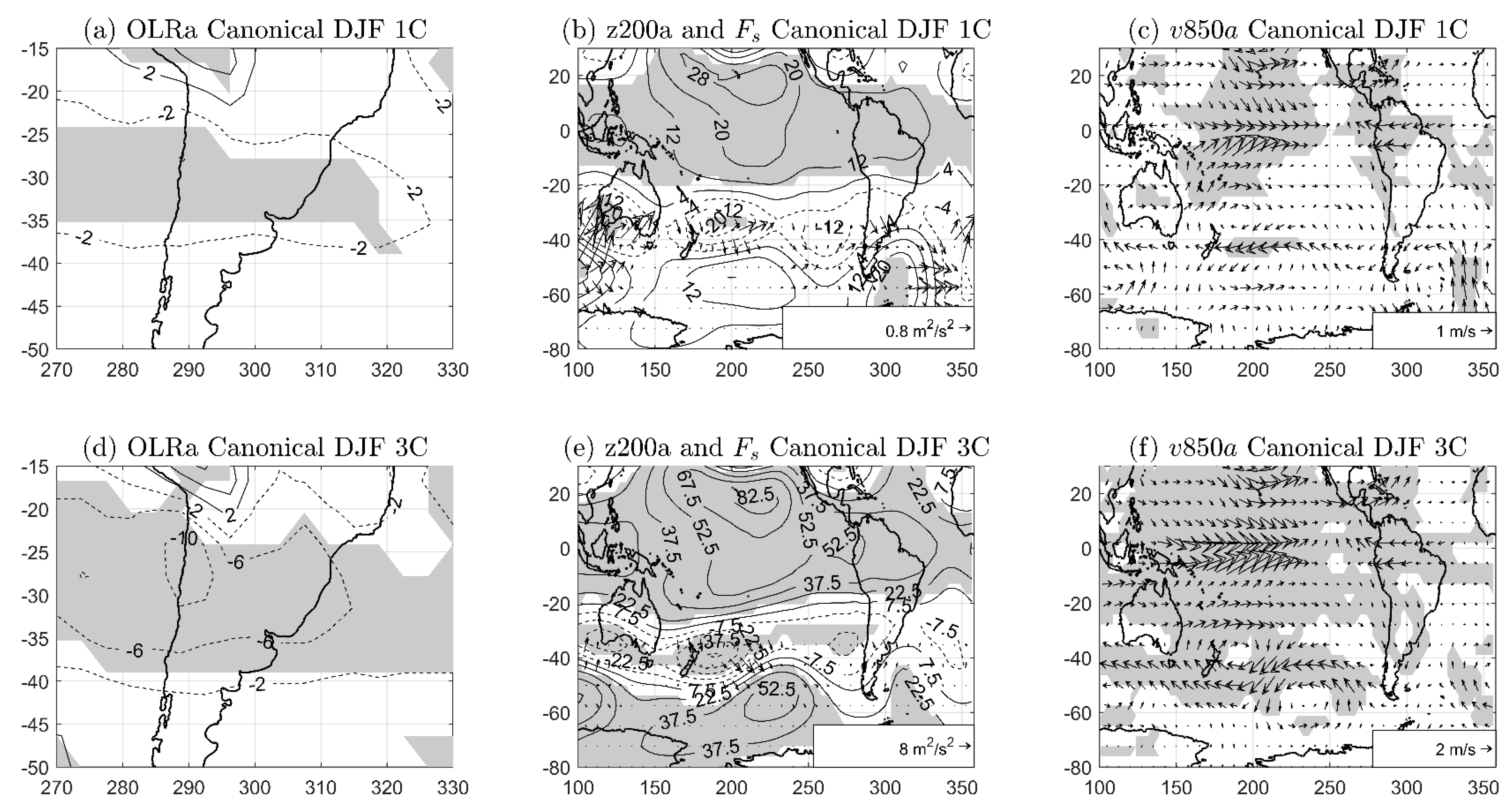
In agreement with observations, the model’s results showed that Canonical_3C experiment induced two Rossby wave trains, a large one that emanated from the subtropical western south Pacific and propagated southeastward, and a shorter one that grew up in the eastern subtropical South Pacific (see Figure 4e). They both presented a barotropic behavior on extratropical latitudes (compare Figure 4e,f), though it was the shorter one that played the main role in generating OLR anomalies over SSA, through (1) an increase of the cyclonic vorticity advection in upper levels, and (2) a strengthening of the northerlies bringing moisture toward SSA at lower levels. Unlike observations, however, the propagation of this shorter Rossby wave train did not show any statistically significant anticyclone over the Atlantic watershed of SSA (compare Figure 2b and Figure 4e).

The comparison of the 1 °C and 3 °C Canonical experiments showed that the increase of the SST anomalies over the eastern equatorial Pacific enhanced the RWS intensity. The statistically significant RWS signal located between Australia and New Zealand (over the western Chilean-Peruvian coast) was related to the generation of the large (short) Rossby wave train. While the larger wave was mainly related to RWS1, the shorter one presented contributions from both RWS1 and RWS2. Finally, the comparison of the z200 anomaly patterns from both Canonical experiments showed that the Speedy response was approximately linear with the increase of the SST anomalies. For the Canonical_1C experiment, the statistically significant reduction of OLR over SSA could be related to the intensification of the upper level jet stream.

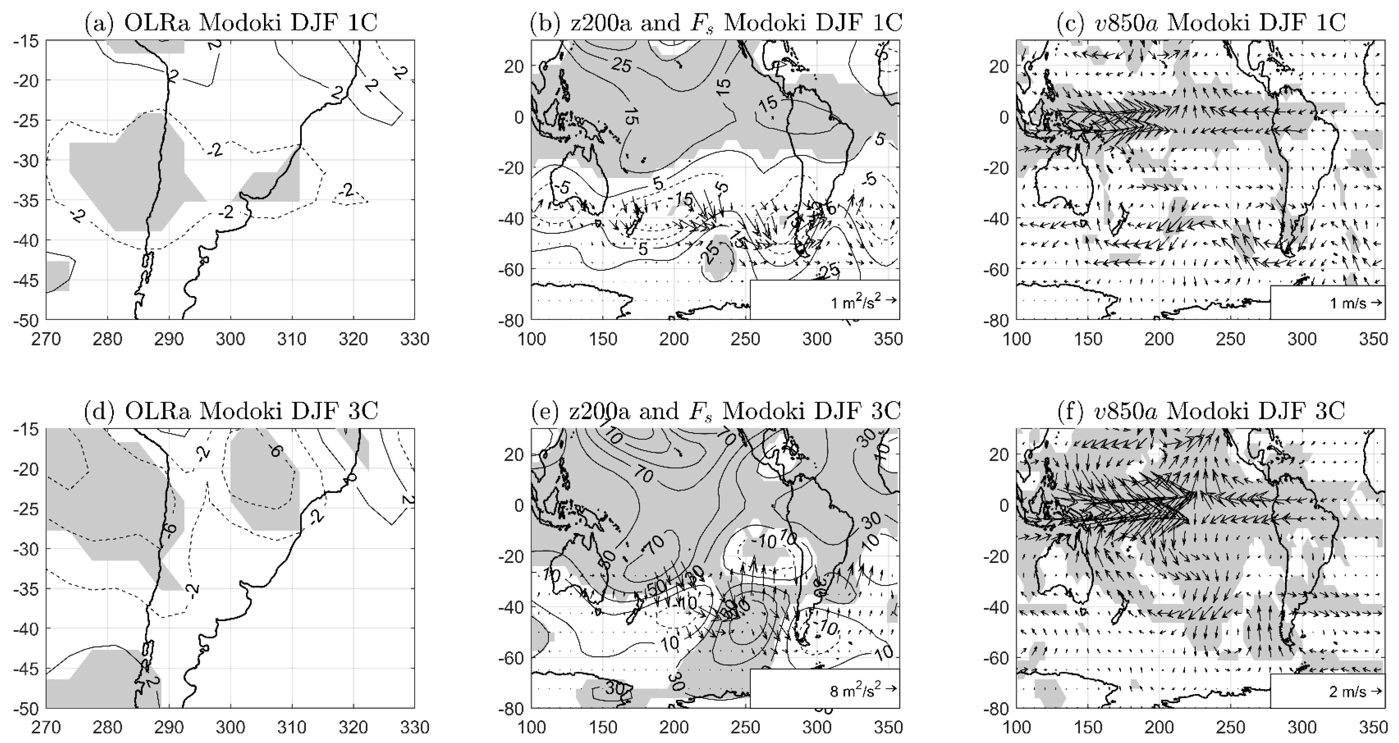
The El Niño Modoki impact on SSA is more debated and there is currently no consensus regarding the influence of this ENSO pattern on SSA. The results from reanalysis here did not show any statistically significant signal over SSA. However, the model’s results showed that the impact of El Niño Modoki on SSA depended on the intensity of the SST anomalies, in such a way that increasing the SST anomalies of this pattern induced statistically significant OLR anomalies over SSA. While El Niño Modoki_1C did not show any statistically significant signal in the z200 anomaly pattern, El Niño Modoki_3C generated a large Rossby wave train that emanated from the subtropical western south Pacific and reached southern SA. The origin of this wave could be related to the negative RWS values developed between Australia and New Zealand (see Figure 6d), whose main contribution came from RWS1 (see Figure 6d,h,l). Finally, unlike Canonical El Niño, the z200 response to El Niño Modoki 3C presented a clear Gill-Matsuno quadrupole response over the tropical atmosphere [34,35] and, comparing El Niño Modoki_1C with 3C, the atmospheric response to this El Niño pattern presented a more non-linear behavior than in the case of Canonical El Niño (compare Figure 5b,e, on the one hand, and Figure 4b,e on the other hand).

Therefore, the model’s results suggested that SSA was more sensitive to SST anomalies over the region of Canonical El Niño, given that the eastern El Niño needed weaker anomalies to induce statistically significant OLR anomalies. In the case of El Niño Modoki, as the atmosphere was less responsive to the SST pattern, it needed larger SST intensities in order to overcome the internal atmospheric variability. This result may have been model dependent and should be tested with other models. Finally, the establishment of teleconnections from the tropics depends on the right simulation of the mean state. Speedy presented a northward bias in the position of the upper level jet (not shown) that could directly influence the wave propagation in the extratropics, and therefore, this could be one reason why Speedy did not present wave propagation until South America for the Canonical El Niño case. Nevertheless, Speedy captured the main dynamics and as an intermediate complexity AGCM it allowed many sensitivity experiments to be performed that have advanced the understanding of teleconnections. Another source of uncertainty could have come from the choice of a particular dataset for the definition of the climatology and spatial patterns that were used for the sensitivity experiments. However, the model’s results shown in this manuscript are consistent with the differing effects of El Niño Modoki over SSA found in the reanalysis and in previous works.

References

1. Cai, W.; Cowan, T. La Niña Modoki impacts Australia autumn rainfall variability. Geophys. Res. Lett. 2009, 36. [Google Scholar] [CrossRef]
2. Grimm, A.M.; Barros, V.R.; Doyle, M.E. Climate variability in southern South America associated with El Niño and La Niña events. J. Clim. 2000, 13, 35–58. [Google Scholar] [CrossRef]
3. King, M.P.; Herceg-Bulić, I.; Bladé, I.; García-Serrano, J.; Keenlyside, N.; Kucharski, F.; Sobolowski, S. Importance of late fall ENSO teleconnection in the Euro-Atlantic sector. Bull. Am. Meteorol. Soc. 2018, 99, 1337–1343. [Google Scholar] [CrossRef]
4. López-Parages, J.; Rodríguez-Fonseca, B.; Terray, L. A mechanism for the multidecadal modulation of ENSO teleconnection with Europe. Clim. Dyn. 2015, 45, 867–880. [Google Scholar] [CrossRef]
5. Ropelewski, C.F.; Halpert, M.S. North American precipitation and temperature patterns associated with the El Niño Southern Oscillation (ENSO). Mon. Weather Rev. 1986, 114, 2352–2362. [Google Scholar] [CrossRef] [Green Version]
6. Kao, H.; Yu, J. Contrasting Eastern-Pacific and Central-Pacific types of ENSO. J. Clim. 2009, 22, 615–632. [Google Scholar] [CrossRef]
7. Xiang, B.; Wang, B.; Li, T. A new paradigm for the predominance of standing central Pacific warming after the late 1990s. Clim. Dyn. 2013, 41, 327–340. [Google Scholar] [CrossRef]
8. Larkin, N.K.; Harrison, D.E. Global seasonal temperature and precipitation anomalies during El Niño autumn and winter. Geophys. Res. Lett. 2005, 32. [Google Scholar] [CrossRef]
9. Ashok, K.; Behera, S.K.; Rao, S.A.; Weng, H.; Yamagata, T. El Niño Modoki and its possible teleconnection. J. Geophys. Res. Oceans 2007, 112. [Google Scholar] [CrossRef]
10. Andreoli, R.V.; Oliveira, S.S.; Kayano, M.T.; Viegas, J.; Souza, R.A.F.; Candido, L.A. The influence of different El Niño types on the South American rainfall. Int. J. Climatol. 2017, 37, 1374–1390. [Google Scholar] [CrossRef]
11. Tedeschi, R.G.; Grimm, A.M.; Cavalcanti, I.F. Influence of Central and East ENSO on extreme events of precipitation in South America during austral spring and summer. Int. J. Climatol. 2015, 35, 2045–2064. [Google Scholar] [CrossRef]
12. Silva, G.A.M.; Ambrizzi, T. Inter-El Niño variability and its impact on the South American low-level jet east of the Andes during austral summer—Two case studies. Adv. Geosci. 2006, 6, 283–287. [Google Scholar] [CrossRef] [Green Version]
13. Weng, H.; Behera, S.K.; Yamagata, T. Anomalous winter climate conditions in the Pacific rim during recent El Niño Modoki and El Niño events. Clim. Dyn. 2009, 32, 663–674. [Google Scholar] [CrossRef]
14. Sun, D.; Xue, F.; Zhou, T. Impacts of two types of El Niño on atmospheric circulation in the Southern Hemisphere. Adv. Atmos. Sci. 2013, 30, 1732–1742. [Google Scholar] [CrossRef]
15. Tedeschi, R.G.; Cavalcanti, I.F.; Grimm, A.M. Influences of two types of ENSO on South American precipitation. Int. J. Climatol. 2013, 33, 1382–1400. [Google Scholar] [CrossRef]
16. Hill, K.J.; Taschetto, A.S.; England, M.H. South American rainfall impacts associated with inter-El Niño variations. Geophys. Res. Lett. 2009, 36. [Google Scholar] [CrossRef]
17. Barreiro, M. Interannual variability of extratropical transient wave activity and its influence on rainfall over Uruguay. Int. J. Climatol. 2017, 37, 4261–4274. [Google Scholar] [CrossRef]
18. Sulca, J.; Takahashi, K.; Espinoza, J.C.; Vuille, M.; Lavado-Casimiro, W. Impacts of different ENSO flavors and tropical Pacific convection variability (ITCZ, SPCZ) on austral summer rainfall in South America, with a focus on Peru. Int. J. Climatol. 2018, 38, 420–435. [Google Scholar] [CrossRef]
19. Brito, A.S. El Niño and El Niño Modoki Impacts on South American Rainfall. Master’s Thesis, The University of New South Wales, Sydney, Australia, 2011. [Google Scholar]
20. Huang, B.; Banzon, V.F.; Freeman, E.; Lawrimore, J.; Liu, W.; Peterson, T.C.; Smith, T.M.; Thorne, P.W.; Woodruff, S.D.; Zhang, H.M. Extended Reconstructed Sea Surface Temperature version 4 (ERSST.v4): Part, I. Upgrades and intercomparisons. J. Clim. 2014, 28, 911–930. [Google Scholar] [CrossRef] [Green Version]
21. Liebmann, B.; Smith, C.A. Description of a Complete (Interpolated) Outgoing Longwave Radiation Dataset. Bull. Am. Meteorol. Soc. 1996, 77, 1275–1277. [Google Scholar]
22. Kanamitsu, M.; Ebisuzaki, W.; Woollen, J.; Yang, S.K.; Hnilo, J.J.; Fiorino, M.; Potter, G.L. Ncep–doe amip-ii reanalysis (r-2). Bull. Am. Meteorol. Soc. 2002, 83, 1631–1644. [Google Scholar] [CrossRef]
23. Li, G.; Ren, B.; Yang, C.; Zheng, J. Indices of El Niño and El Niño Modoki: An improved El Niño Modoki index. Adv. Atmos. Sci. 2010, 27, 1210–1220. [Google Scholar] [CrossRef]
24. Molteni, F. Atmospheric simulations using a GCM with simplified physical parameterizations. I: Model climatology and variability in multi-decadal experiments. Clim. Dyn. 2003, 20, 75–191. [Google Scholar] [CrossRef]
25. Kucharski, F.; Molteni, F.; Bracco, A. Decadal interactions between the western tropical Pacific and the North Atlantic Oscillation. Clim. Dyn. 2006, 26, 79–91. [Google Scholar] [CrossRef]
26. Barreiro, M.; Diaz, N. Land-atmosphere coupling in El Nino influence over South America. Atmos. Sci. Lett. 2011, 12, 351–355. [Google Scholar] [CrossRef]
27. Barreiro, M.; Diaz, N.; Renom, M. Role of the global oceans and land-atmosphere interaction on summertime interdecadal variability over northern Argentina. Clim. Dyn. 2014. [Google Scholar] [CrossRef]
28. Saravanan, R.; Chang, P. Interaction between tropical Atlantic variability and El Niño-Southern Oscillation. J. Clim. 2000, 13, 2177–2194. [Google Scholar] [CrossRef]
29. Barreiro, M.; Tippmann, A. Atlantic modulation of El Nino influence on summertime rainfall over Southeastern South America. Geophys. Res. Lett. 2008, 35. [Google Scholar] [CrossRef] [Green Version]
30. Barreiro, M. Influence of ENSO and South Atlantic Ocean on climate predictability over southeastern South America. Clim. Dyn. 2010, 35, 1493–1508. [Google Scholar] [CrossRef]
31. Plumb, R.A. On the three-dimensional propagation of stationary waves. J. Atmos. Sci. 1985, 42, 217–229. [Google Scholar] [CrossRef]
32. Martín-Gómez, V.; Barreiro, M. Analysis of oceans’ influence on spring time rainfall variability over Southeastern South America during the 20th century. Int. J. Climatol. 2015, 36, 1344–1358. [Google Scholar] [CrossRef]
33. Hill, K.J.; Taschetto, A.S.; England, M.H. Sensitivity of South American summer rainfall to tropical Pacific Ocean SST anomalies. Geophys. Res. Lett. 2011, 38. [Google Scholar] [CrossRef] [Green Version]
34. Taschetto, A.S.; Haarsma, R.J.; Gupta, A.S.; Ummenhofer, C.C.; Hill, K.J.; England, M.H. Australian monsoon variability driven by a Gill–Matsuno-type response to central west Pacific warming. J. Clim. 2010, 23, 4717–4736. [Google Scholar] [CrossRef] [Green Version]
35. Kucharski, F.; Bracco, A.; Yoo, J.H.; Tompkins, A.M.; Feudale, L.; Ruti, P.; Dell’Aquila, A. A Gill–Matsuno-type mechanism explains the tropical Atlantic influence on African and Indian monsoon rainfall. Q. J. R. Meteorol. Soc. A J. Atmos. Sci. Appl. Meteorol. Phys. Oceanogr. 2009, 135, 569–579. [Google Scholar] [CrossRef]
Figure 1. (a) Subtropical South America (SSA) domain; (b) regression map of Niño3 index onto sea surface temperature (SST) anomalies over the period (1979–2016); (c) regression map of El Niño Modoki index onto SST anomalies over the period (1979–2016). Both indices and anomalies are centered on December-January-February (DJF).
Atmosphere 11 00077 g001
Figure 2. Correlation maps for Canonical El Niño (first row) and El Niño Modoki (second row). Correlation of outgoing longwave radiation (OLR)a (a,d); z200a (b,e); and v850a (c,f). Shaded regions exceed the 95% level of confidence from a two-tailed t-test. OLRa units: W/m2, z200a units: m and v850 units: m/s. Results from reanalysis data.
Atmosphere 11 00077 g002
Figure 3. Composite z200 anomaly map for (a) Canonical El Niño and (b) El Niño Modoki. Vectors represent the Fs field. Shaded regions exceeded the 95% level of confidence from a two-tailed t-test. z200a units: m, v850 units: m/s and Fs units: m2s2. Results from reanalysis data.
Atmosphere 11 00077 g003
Figure 4. Model response to the Canonical El Niño 1 °C (first row) and Canonical El Niño 3 °C (second row) in (a,d) OLRa, (b,e) z200a (contours) and Fs (arrows), and (c,f) v850a. Such response was obtained by subtracting the ensemble mean of the CONTROL experiments to the ensemble mean of the El Niño type experiments (Canonical_1C or Canonical_3C). Shaded regions exceeded the 95% level of confidence from two-tailed t-test. OLRa units: W/m2, z200a units: m, Fs units: m2s−2 and v850 units: m/s.
Atmosphere 11 00077 g004
Figure 5. Model response to El Niño Modoki_1C (first row) and El Niño Modoki_3C (second row). (a,d) OLRa, (b,e) z200a and Fs, and (c,f) v850a. Maps were obtained by subtracting the ensemble mean of the CONTROL experiments to the ensemble mean of the El Niño type experiments (Modoki_1C or Modoki_3C). Shaded regions exceeded the 95% level of confidence from two-tailed t-test. OLRa units: W/m2, z200a units: m, Fs units: m2s−2 and v850 units: m/s.
Atmosphere 11 00077 g005
Figure 6. Composite maps of the Rossby Wave Sources (RWS)a (s−2). First and third columns show results for Canonical_1C and Modoki_1C experiments, respectively. Second and fourth columns show the results for Canonical_3C and Modoki_3C experiments. In (ad) the whole RWS field is shown. (eh) shows the vortex stretching term (RWS1), and (il) the advection of absolute vorticity by the divergent wind flow (RWS2). Values are multiplied by the scale factor 10−10. Shaded regions exceeded the 95% level of confidence from two-tailed t-test.
Atmosphere 11 00077 g006