Abstract
Air quality modeling at the very local scale within an urban area is performed through a hybrid modeling system (HMS) that combines the CAMx Eulerian model the with AUSTAL2000 Lagrangian model. The enhancements obtained by means of the HMS in the reconstruction of the spatial distribution of fine particles (PM2.5) and elemental carbon (EC) concentration are presented for the case-study of Milan city center in Northern Italy. Modeling results are reported for three receptors (a green area, a residential and shopping area, and a congested crossroad on the inner ring road of the city center) selected in order to represent urban sites characterized by both different features in terms of the surrounding built environment and by different exposure to local emission sources. The peculiarity of the three receptors is further highlighted by source apportionment analysis, developed not only with respect to the kind of emission sources but also to the geographical location of the sources within the whole Northern Italy computational domain. Results show that the outcome of the Eulerian model at the local scale is only representative of a background level, similar to the Lagrangian model’s outcome for the green area receptor, but fails to reproduce concentration gradients and hot-spots, driven by local sources’ emissions.
Keywords:
air quality; hybrid modeling; source apportionment; source regions; CAMx; AUSTAL2000; Milan; Po valley 1. Introduction
Air pollution in urban areas is a significant public health issue because of chronic diseases, principally of respiratory and cardiovascular nature [1], and because of premature deaths resulting from population exposure to atmospheric pollutants [2,3,4]. According to Lelieveld et al. [5], the loss of life expectancy due to air pollution is higher than those caused by tobacco smoking and AIDS. In 2015, air pollution-related diseases were estimated to be responsible for about 6.4 million premature deaths worldwide, with 4.2 million due to ambient air pollution. Indeed, during that year, about 90% of the population, mostly people living in cities, was exposed to particulate matter in concentrations exceeding the WHO air quality guidelines [2]. Air quality monitoring networks provide data in order to check the compliance with air quality limits. However, monitoring sites are usually limited in number and, even though located at sites supposedly representative of different urban microenvironments, their data may not properly assess the actual air quality over the whole urban area [6].
Air quality models are useful tools to assess pollutant concentration levels and emission sources’ contributions in urban areas [7,8,9]. Situations where models can be applied for air quality assessment instead of, or in combination with fixed measurements have been defined by the European Union Directive 2008/50 on air quality [10]. Moreover, most of models can support epidemiological studies providing concentration data with high spatial and temporal resolution for exposure assessment of selected individuals, allowing both predictions on future exposure and reconstruction of historical exposure [11].
However, air quality modeling in urban areas is quite challenging for a number of reasons:
- –
- The concentration levels of atmospheric pollutants are the result of three additional contributions: a regional background (i.e., the baseline level in the surroundings/region of the urban area); an urban background, representing the increment of concentration due to emission of the urban area itself; and a very local contribution of emission sources at pollution hotspots within the urban area [12].
- –
- The pollutants of interest may be not only of primary origin (i.e., directly emitted by emission sources) but also the result of secondary formation processes, like those affecting O3, NO2, and fine particulate matter.
- –
- The spatial distribution of the emission sources in urban areas, essentially road traffic and space heating, depends on the urban structure of the built environment, that, in turn, can affect the dispersion of the locally emitted polluted, with local modifications of the wind conditions induced by buildings and with urban canyon structures favoring the build-up of pollutants at emission hot-spots [13].
- –
- Last but not least, model reliability strongly depends on both emission data accuracy, spatial resolution and temporal modulation [14,15,16,17], and on the proper reconstruction of the meteorological conditions driving the motion of air masses and pollutant transport and diffusion [18,19].
Eulerian chemical and transport models (CTMs) are commonly applied for air quality modeling at the regional scale, reasonably well estimating regional and urban background concentration levels for both primary and secondary pollutants. Conversely, they are not able to properly reproduce the local concentration gradients in urban areas due to the relatively large step of the computational grid. In order to overcome this limitation, various modeling frameworks that integrate CTMs outputs with other models have been proposed for better reproducing within-city exposure variability. Geostatistical approaches combining land use regression (LUR) and chemical transport modeling have been proposed for long-term concentrations of NO2, O3 and particulate matter [20,21,22,23,24]. Hybrid deterministic models combining a Lagrangian dispersion model (LDM) at the local scale and a CTM at the regional scale have been proposed for NOX and PM10 [25,26,27]. Indeed, LDMs can be profitably used for the assessment of local sources’ impact at high spatial resolution over a small domain because of the fine computational grid that allows a more realistic spatialization of urban emissions, depending on the road network layout and the built environment structure, also accounting for wind field modifications induced by buildings [28]. As drawbacks, LDMs do not include comprehensive gas and aerosol chemistry modules for secondary pollutants assessment and cannot be used for regional scale modeling due to their computational burden.
This work is focused on air quality modeling at the very local scale within an urban area through a hybrid modeling system that combines the CAMx (Comprehensive Air quality Model with Extensions) Eulerian model with the AUSTAL2000 Lagrangian model. In particular, the work highlights the enhancements in the reconstruction of the spatial distribution of the concentration of fine particles (PM2.5) and elemental carbon in the city center of Milan, obtained by means of the hybrid modeling system in comparison with the CAMx Eulerian model. The city of Milan, located in the Po valley in Northern Italy, is a well-known hotspot for particulate matter (PM) pollution. Modelling results are presented for three receptors selected in order to represent urban sites characterized by both different features in terms of the surrounding built environment and by different exposure to the local emission sources. The peculiarity of the three receptors is further highlighted by the source’s apportionment analysis developed not only with respect to the kind of emission sources but also to the geographical locations of the sources within the whole Po valley computational domain.
2. Methods
2.1. HMS Modeling Chain Setup
The hybrid modeling system (HMS) used for air quality simulations and source apportionment analysis is composed by three main components (Figure 1): the Weather Research and Forecasting meteorological model (WRF v3.4.1; [29]), the Comprehensive Air quality Model with Extensions (CAMx v6.30; [30]), as Eulerian chemical and transport model, and AUSTAL2000 (AUSTAL2000 v2.6.9; [31]), as Lagrangian local-scale model. The HMS setup also includes the Sparse Matrix Operator for Kernel Emissions model (SMOKE v3.5; [32]) for emission inventory data processing. CAMx was coupled with AUSTAL2000 in order to better estimate concentration levels and properly assess sources’ contribution over the urban local domain, thanks to the strong refinement in the spatialization of local emissions according to the road network layout (for traffic emissions) and of the built environment structure (for commercial and residential combustion emissions).
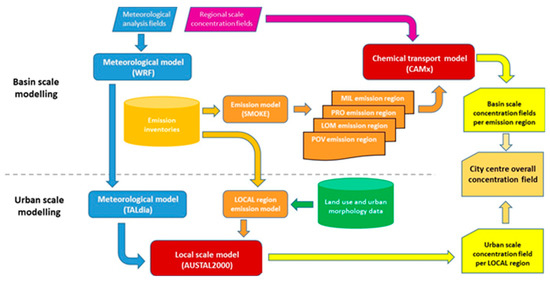
Figure 1.
Hybrid modeling system setup.
Input meteorological fields for 2010 were reconstructed by the WRF model, driven by ECMWF (European Centre for Medium-Range Weather Forecasts) analysis fields, “Operational Atmospheric Model Data Set class = od − ANA”, at all hours available (00:00, 06.00, 12:00, 18:00 GMT), and set up with 30 vertical layers spanning from 25 m up to 15 km above the ground. Initial and boundary conditions from ECMWF analysis fields, at 0.5° × 0.5° grid size, included 3D (wind speed components, temperature, relative humidity) and 2D surface parameters (sea level pressure and temperature), 2D static parameter for land-sea mask, and 3D soil parameters (temperature and water content), integrated on 4 ground layers (0–7 cm, 7–28 cm, 28 cm–1 m, 1–2.55 m). Horizontally, four nested grids covering Europe, Italy, Po valley, and Milan metropolitan area have been used; grid resolutions are 45 km, 15 km, 5 km, and 1.7 km, respectively. WRF model evaluation was discussed in Pepe et al. [26], with respect to both the Po valley and Milan metropolitan area; the time series of observed and computed values of mixing ratio, temperature and wind speed over Milan metropolitan area are reported in Supplementary Material Figure S1. The wind rose for calendar year 2010 at Milano Linate airport is presented in Figure S2.
CAMx simulations covered the two innermost domains of WRF (Po valley and Milan metropolitan area). CAMx was run at the same spatial resolution of WRF, but with a slight reduction of the domains in order to remove boundary effects (Supplementary Material Table S1). AUSTAL2000 simulation covered one single cell (1.7 × 1.7 km2) of CAMx Milan metropolitan area domain with 20 m grid resolution. This cell covers part of Milan city center and is characterized by a heterogeneous urban pattern with road arches separating the densely built up commercial and residential areas (Figure 2).
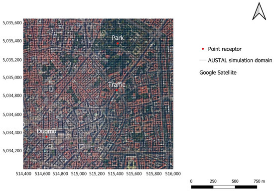
Figure 2.
AUSTAL2000 computational domain over Milan city center and selected receptors location.
Input meteorological fields for AUSTAL2000 were calculated by the diagnostic wind field model TALdia based on WRF model output and on the urban canopy features at 20 × 20 m2 resolution, according to the European land use atlas data [33].
Emissions were derived from inventory data at three different spatial resolution levels: European Monitoring and Evaluation Programme data (EMEP) [34], available over a regular grid of 50 × 50 km2; ISPRA Italian national inventory data [35] which provides a disaggregation for province; regional inventories data based on INEMAR (INventario EMissioni ARia) methodology [36] for the administrative regions of Lombardy, Veneto and Piedmont, which provide detailed emissions data at single municipality level. Data from each emission inventory were processed using the SMOKE model in order to obtain the hourly time pattern of the emissions. Further details on WRF, CAMx, AUSTAL2000 setup, on meteorological and emissions input data, and on the chemical schemes adopted in this work are reported in Pepe et al. [26], together with the model validation phase for the 2010 calendar year through the comparison between model results and measurements at air quality stations.
2.2. Emission Regions and Emission Categories
HMS source apportionment analyses concurrently considered different emission categories (e.g., road transport, disaggregated by vehicles type, commercial and residential combustion, disaggregated by fuel used) and emission regions i.e., user-defined areas of particular interest for administrative reasons or for the location of specific emission sources. Thus, thanks to the Particulate matter Source Apportionment Technology, (PSAT) algorithm [37], embedded in CAMx, source apportionment analyses could detect contributions from emission categories in combination with geographic information on source locations. The key feature introduced by HMS is the higher detail of source apportionment analysis at urban receptors, where the contributions due to local sources (i.e., located in proximity of the receptors), not correctly disaggregated by CAMx with consequent inaccuracies for source apportionment analyses, are properly accounted for by AUSTAL2000, conversely. In this work, 11 emission categories (Table S2) and 5 emission regions over the Po Valley are considered for the source apportionment (Figure S1). Together with a local urban region (LOCAL), covering the CAMx cell in Milan city center corresponding to the AUSTAL2000 domain, four nested emission regions have been defined: the MIL region covers the municipality of Milan, the PRO region the metropolitan area of Milan, the LOM region the Lombardy region, and the POV region the Po valley. Each emission region accounts for the sources located within its boundaries except those located in the nested inner domains. Additionally, a sixth region that considers sources located within the computational domain but outside of Italy and long-range transport was included in source apportionment analyses. Further details about emission categories and region maps are illustrated in Pepe et al. [25].
2.3. HMS Source Apportionment Output
The HMS approach has been applied in order to assess fine particles (PM2.5) and elemental carbon (EC) ambient concentration levels and related source contributions at three receptors in Milan city center. PM2.5 is one of the regulated pollutants of major concern, due to its health relevance and to its rather high average and episodic concentration levels, especially during the winter months. EC is a primary component of PM particularly critical for human health [38]. The three receptors, all located within the same cell of CAMx’s innermost domain (Figure 2), which corresponds to AUSTAL2000 computational domain, were selected in order to represent sites with a different exposure to the local emission sources. Namely, they correspond to a green area (PARK), to a residential and shopping area near the main cathedral square (DUOMO), and to a congested crossroad on the inner ring road of the city center (TRAFFIC). Such a selection was also intended to highlight the capability of AUSTAL2000 for a more reliable source apportionment at the local scale in comparison with CAMx.
Double counting of the emissions from the LOCAL region was avoided thanks to the PSAT source apportionment that allowed to track separately the contributions of the emission regions to the total concentration computed by CAMx. HMS concentration values and source apportionment results at the selected receptors are the combination of CAMx results for the emissions from the most part of the Po valley computational domain (i.e., from POV, LOM, PRO, and MIL region) and of AUSTAL2000 results for the LOCAL region.
3. Results and Discussion
All model results refer to the three abovementioned urban receptors and consider both PM2.5 and EC, focusing on the following issues: (i) AUSTAL2000 output, that is concentration levels and related contribution for the emission sources in the LOCAL region; (ii) comparison between AUSTAL2000 and CAMx output for the concentration levels and for the contributions of the emission sources from the LOCAL region; (iii) HMS concentration levels and sources’ contributions for the emissions from the whole Po valley computational domain, also accounting for the geographical locations of the sources (i.e., emission regions).
3.1. AUSTAL2000 Output
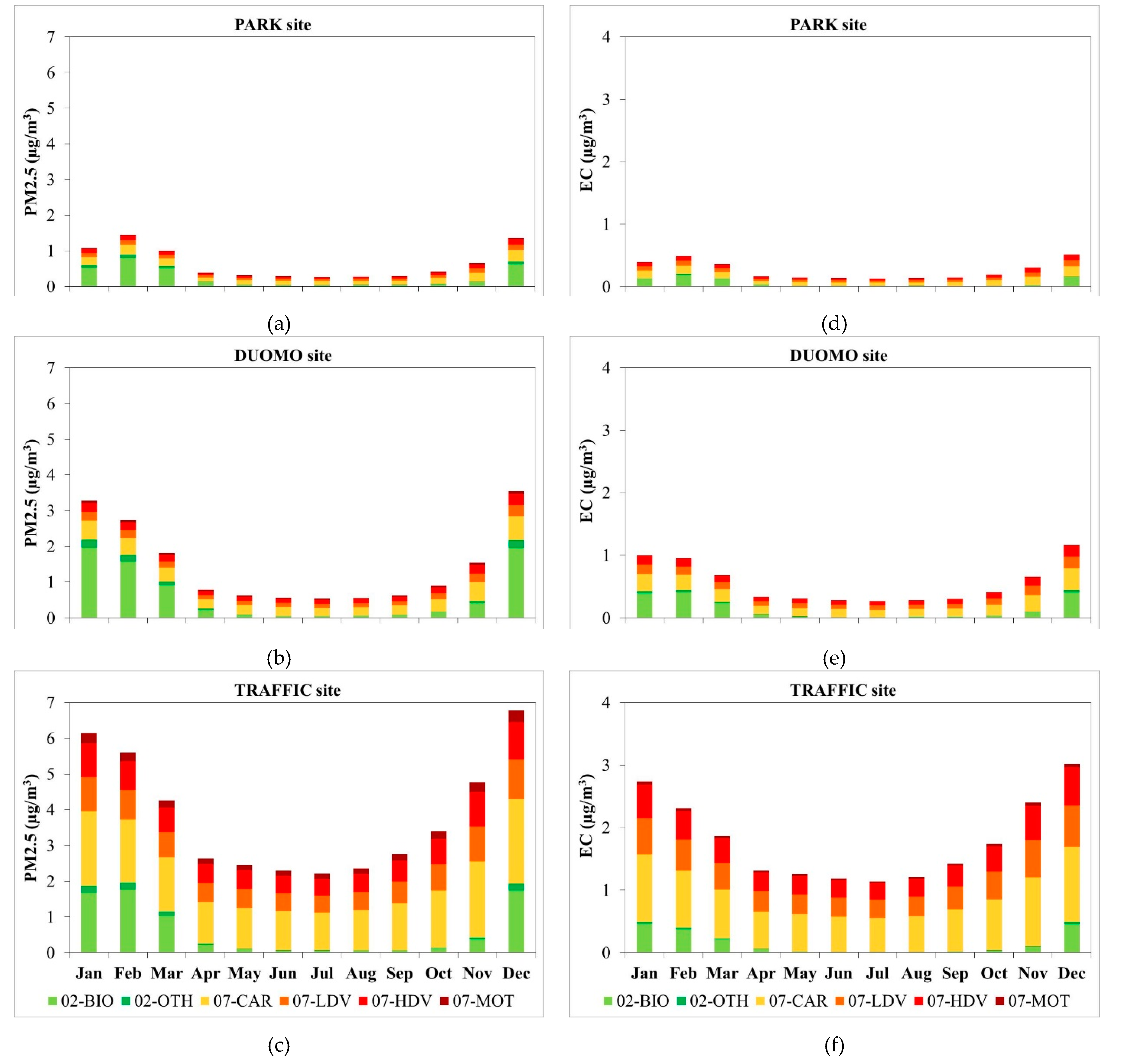
This section provides an overview of AUSTAL2000 source apportionment results for PM2.5 and elemental carbon (EC) emitted by local sources of the innermost computational domain (LOCAL region). AUSTAL2000 simulations for PM2.5 consider only its primary fraction (PPM2.5) because the model does not handle aerosol chemistry; that at the very small spatial scale the secondary PM generated by the local emissions of precursors is substantially negligible [39]. According to emission inventory data, commercial and residential combustion (C&R combustion–SNAP category 02) and road traffic (SNAP category 07) are responsible for more than 90% of the emissions within the domain; thus, for the LOCAL region this work is focused on the contributions to ambient levels from these two source categories. Estimated contributions to ambient PM2.5 and EC levels at the three receptors are presented in the panels of Figure 3 as monthly average values for calendar year 2010, with a breakdown based on both source categories and sub-categories (i.e., kind of fuel for C&R combustion, vehicle class for road traffic). Relative contributions, assessed both on annual basis and for the cold and warm season separately, for a deeper insight on seasonality of sources’ activity, are summarized in Table 1 for PM2.5 and in Table 2 for EC.

Figure 3.
Monthly contributions of C&R combustion and road traffic emissions from the LOCAL area to primary PM2.5 (left column: (a) PARK site; (b) DUOMO site; (c) TRAFFIC site) and EC (right column: (d) PARK site; (e) DUOMO site; (f) TRAFFIC site) ambient levels at the three urban receptors for 2010.

Table 1.
Total annual and seasonal average contributions to PM2.5 ambient levels and percentage contributions of emission sources in the LOCAL area at the three urban receptors. (02-BIO: Residential and commercial heating-Biomass burning; 02-OTH: Residential and commercial heating-Fossil fuels burning; 07-CAR: Road traffic-Passenger cars; 07-LDV: Road traffic-Light Duty Vehicles; 07-HDV: Road traffic-Heavy Duty Vehicles; 07-MOT: Road traffic-Mopeds and motorcycles).

Table 2.
Total annual and seasonal average contributions to EC ambient levels and percentage contributions of emission sources in the LOCAL area at the three urban receptors.
3.1.1. PM2.5
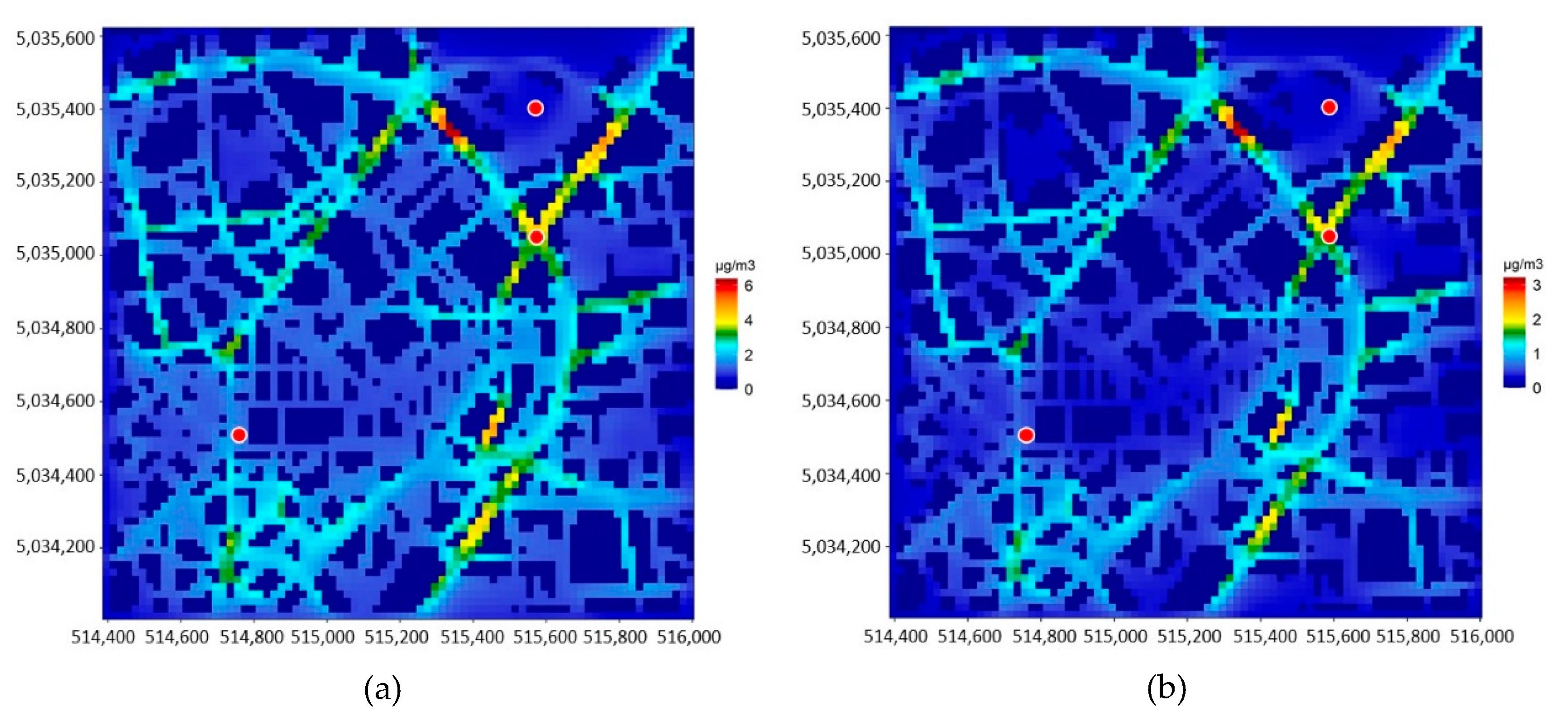
PM2.5 results account only for primary PM2.5 because the local scale model AUSTAL2000 does not include a chemical module, thus neglecting chemical transformation process of gaseous precursors that lead to secondary particle formation. The map of the spatial distributions of PM2.5 annual mean concentration over AUSTAL2000 simulation domain (Figure 4a) clearly displays the model ability to account for the structure of the built environment, namely with respect to the main road network. Because of the different exposure to the LOCAL region sources, quite different concentrations levels are estimated for the selected receptors, as expected (0.65 µg/m3, 1.46 µg/m3, and 3.80 µg/m3 at PARK, DUOMO, and TRAFFIC receptor, respectively).
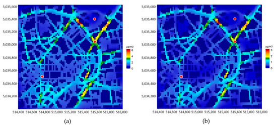
Figure 4.
Spatial distribution of PM2.5 (a) and EC (b) annual mean concentrations generated by LOCAL source emissions over AUSTAL2000 computational domain.
At PARK receptor the overall contribution of the local sources displays a clear seasonal pattern (Figure 3a), with higher contribution in the cold season (>1 µg/m3 from December to March) and lower contributions in the warm season (<0.5 µg/m3 from April to October). Peaks up to about 1.5 µg/m3 are estimated in February and December and the lowest concentrations (about 0.25 µg/m3) from June to August. The pattern is mainly driven by the seasonality that affects sources’ activity, with emissions from C&R combustion in addition to traffic emissions in the cold season. C&R combustion, namely biomass burning (02-BIO), is the first contributor among local sources with a contribution ranging between 0.5 µg/m3 and 0.9 µg/m3; conversely, it is almost negligible in the warm season when its contribution is about 0.04 µg/m3. Road traffic contribution is rather constant throughout the year (ranging between 0.25 µg/m3 and 0.5 µg/m3). In the cold season (January–March), 58.2% of PM2.5 from local sources comes from C&R combustion (category 02), mostly from biomass burning (52.3%); in the warm season (July–September), its contribution drops down to 16.2%, still almost entirely due to biomass combustion (14.5%). Road traffic is responsible for 41.9% of PM2.5 mass in the cold season and for 83.8% in the warm season. However, notwithstanding the higher values computed during winter for C&R combustion, on annual basis road traffic (57.1%) prevails on domestic heating (42.9%). In details, on annual basis passenger cars contribute for almost half of the road traffic share (27.8%), light- and heavy-duty vehicles produce almost the same contribution (13% each), while mopeds and motorcycles account for about 4%.
At DUOMO receptor the overall contribution of the local sources follows the same seasonal pattern observed at PARK site, but concentration levels are twice as high in each month (Figure 3b). During the winter months the total contribution generated by vehicles and heating is always in excess of 1.5 µg/m3, but even higher than 3 µg/m3 in January and up to 3.5 µg/m3 in December. From April to October PM2.5 levels are always below 0.9 µg/m3, but they are around 0.5 µg/m3 from June to August. In spite of the limited distance between PARK and DUOMO receptor (less than 2 km as crow fly distance) the model is able to reproduce the concentration gradient due to the activity of very local sources active in the neighborhoods of the residential DUOMO site. As for the PARK receptor, the biomass burning contribution prevails over road traffic during the winter period while the latter takes over during summer. Contribution from sub-category 02-BIO is in the 1–2 µg/m3 range in the cold season but falls down to about 0.05 µg/m3 in the warm season; road traffic contribution ranges between summer values around 0.5 µg/m3 and winter values up to 1.3 µg/m3. Relative contributions show seasonal figures similar to those of PARK receptor: in the cold season, category 02 accounts for 63.3%, with a 56.9% from biomass burning, in the warm season for 11.9%, again almost entirely due to biomass combustion (10.7%); road traffic is responsible for 36.7% of PM2.5 mass in the cold season and for 88% in the warm season, a few percentage points more than at the PARK receptor, coherently with the higher exposure to traffic emission of the DUOMO receptor. Thus, on annual basis the two sources categories provide almost equal contributions to ambient PM2.5: road traffic contributes for 52.2%, with vehicle classes’ share similar to those of the PARK site (25.5% from passenger cars, about 11.5% from light- and heavy-duty vehicles, and 3.5% from mopeds and motorcycles) and C&R combustion generates the remainder 47.8%.
At TRAFFIC receptor the monthly time series of estimated contributions shows the same seasonal pattern as at the two previous sites, but with values 4 to 8 times higher than at the PARK receptor and roughly 2 to 4 times higher than at DUOMO receptor (Figure 3c). During the winter months the local sources is always in excess of 4 µg/m3, but even higher than 6 µg/m3 in January and December; from April to September, PM2.5 levels are always in the 2–3 µg/m3 range. The highest contribution (6.8 µg/m3 in December) is about 5× and 2× the contribution estimated at PARK and DUOMO receptors in the same month; the lowest (2.2 µg/m3 in July) is 8× and 4× the contributions estimated at the latter sites. Differently from PARK and DUOMO, road traffic is the main contributor not only in the warm season but also in the cold season. Estimated contribution from traffic are in the 4–5 µg/m3 range in wintertime and about 2.5 µg/m3 in summertime; C&R combustion contribution is in the same order as at DUOMO (2 µg/m3) in wintertime and becomes practically insignificant in summertime (<0.06 µg/m3) as for the other two receptors. Actually, in the warm season the contribution of C&R combustion to primary PM2.5 is almost negligible (3%), the remainder 97% coming from road traffic. In the cold season, the overall contribution of category 02 rises up to 31.1% (27.9% from biomass burning) but still largely ancillary with respect to road traffic, and even to the contribution of passenger cars alone (33.6%). On an annual, basis traffic is responsible for 82.3% of annual mean concentration with 40% due to passenger cars, 18.5% from light- and heavy-duty vehicles, and 5% from mopeds and motorcycles; the residual 17.7% is described by C&R combustion, once again almost entirely due to biomass burning (15.9%).
It is worth noting that the contribution of C&R combustion to primary PM2.5 due to LOCAL sources is probably affected by a partial overestimation because of both the spatial disaggregation and temporal modulation procedures. Indeed, due to the limitation on proxy data for emission spatialization, the emission density was kept constant at municipality level, meaning that it was not possible discriminate differences among Milan city center (i.e., LOCAL region) and the city outskirts (i.e., MIL region). Thus, a possible overestimation of the total emission of biomass burning in the LOCAL cell could have taken place. Furthermore, due to a limitation of the data availability C&R combustion emissions were modulated using a unique profile, more representative of domestic heating than of commercial activities. As a consequence, commercial activity emissions, such as wood oven pizzerias, that are the prevailing source of primary PM for non-residential biomass burning in SNAP category 02, are probably overestimated during the winter season.
3.1.2. EC
Results for EC confirm that the model is able to reproduce the seasonality that affects both sources’ activity and atmospheric dispersion, as well the spatial variability of sources’ contributions within the urban area due to the different exposure to emission sources of the receptor sites. Seasonality effects are pointed out by the same U-shaped pattern as primary PM2.5 computed at all sites for the time series of monthly EC contributions and by the higher EC/PM2.5 ratios in the warm season, when road traffic is practically the only contributor to PM2.5 levels. Site-dependent exposure to emission sources, unevenly distributed in the urban area because of the features of the built environment and of the road network, is highlighted by the different concentration levels and related gradients at the very local scale (Figure 4b). Indeed, the EC annual mean concentrations estimated at PARK, DUOMO, and TRAFFIC (0.26 µg/m3, 0.55 µg/m3, and 1.80 µg/m3, respectively) reflect their different exposure to the traffic emission of the LOCAL region sources.
At PARK receptor EC levels are in the 0.13–0.14 µg/m3 and in the 0.4–0.5 µg/m3 range during the warm and cold season, respectively (Figure 3d). As for primary PM2.5, road traffic is the main contributor (>90%) in the warm season but, differently, it is also the main contributor in the cold season (62.5%); on annual basis, local traffic is responsible for 75.5% of ambient EC, the remainder 24.5% almost entirely due to biomass burning in C&R combustion processes (22.9%) (Table 2). The breakdown of road traffic contribution by vehicle class shows figures similar to those of primary PM2.5 but with a slightly higher share (few % points) for light- and heavy-duty vehicles, all powered by diesel engines.
Similar considerations hold for the DUOMO receptor despite the fact that, as for PM2.5, monthly concentration levels are 2×–3× higher than at PARK (Figure 3e), ranging between 0.27 and 0.42 µg/m3 and 0.7 and 1.2 µg/m3 during the warm and cold season, respectively. Like at the PARK receptor, road traffic is the first contributor on both seasons, responsible for 57.4% in wintertime and 94.1% in summertime, with the contribution of passenger cars almost equal to Light Duty Vehicles (LDV) and Heavy Duty Vehicles (HDV) contributions altogether.
At the TRAFFIC receptor, monthly EC levels are 4 to 10 times higher than at the PARK receptor and 2.4 to 4.6 times higher at DUOMO (Figure 3f), thus pointing out spatial gradients even larger than for PM2.5, as a consequence of the greater exposure to primary emissions from traffic. Estimated EC values are in the 1.2–3 µg/m3 range, averaging about 2.3 µg/m3 and 1.3 µg/m3 in wintertime and summertime, respectively, and leading to an annual average of 1.8 µg/m3. Road traffic is by far the main contributor to EC levels (cold season: 83.8%; warm season: 98.7%; annual basis 91.2%) with single SNAP 07 sub-categories contributions prevailing on biomass burning (02-BIO) even in the cold season (Table 2).
3.2. Comparison between AUSTAL2000 and CAMx Output
Results for ambient PM2.5 and EC levels estimated by AUSTAL2000 have been compared to the corresponding estimates provided by CAMx for the three receptors of the urban area in order to point out the accuracy increase that can arise from coupling the local-scale Lagrangian approach with the mesoscale Eulerian approach within the hybrid modeling system. Actually, CAMx (Eulerian approach) is able to reproduce the large part of chemical processes in the atmosphere, including the secondary formation of aerosols, but has a limited spatial resolution; conversely, AUSTAL2000 (Lagrangian approach) is expected to reconstruct more faithfully the spatial resolution of concentrations, though neglecting chemical transformations.
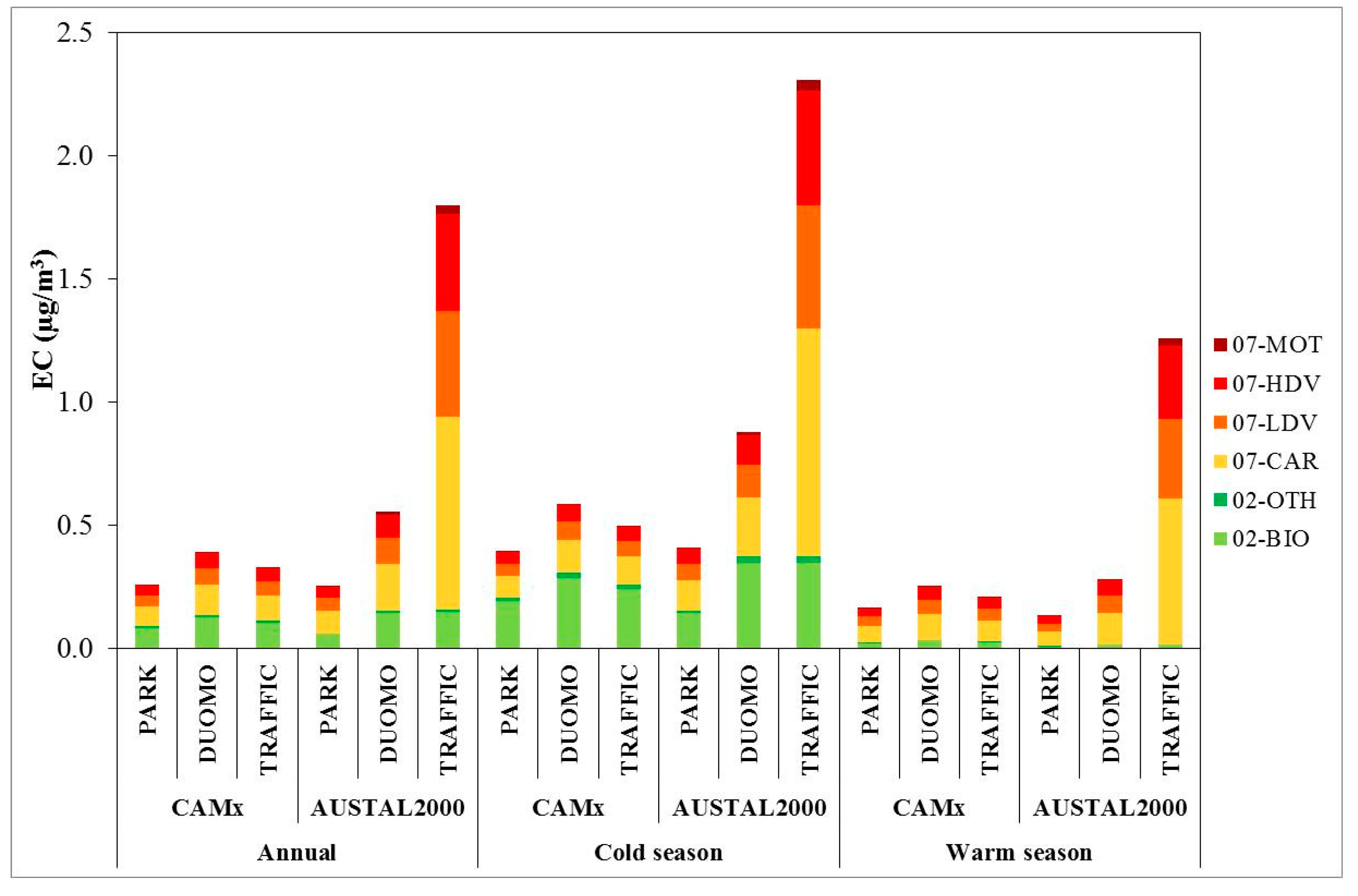
Local sources’ contributions and source apportionment results at the three urban receptors from CAMx and AUSTAL2000 runs are compared in Figure 5 for primary PM2.5 and in Figure 6 for EC. Comparisons, presented for both annual and seasonal average concentrations, point out the relatively “flat” output of CAMx with very limited spatial variability of PPM2.5 and EC concentration levels, notwithstanding the radical change of features of the urban receptors. Conversely, AUSTAL2000 results highlight the difference between the receptor strongly affected by local sources (TRAFFIC) and the receptors less exposed to traffic emissions (DUOMO) and in an urban background location (PARK). PPM2.5 concentrations estimated by CAMx vary in rather narrow ranges (0.7–1.1 µg/m3 in wintertime, 0.3–0.4 µg/m3 in summertime) whereas AUSTAL2000 results display variations in the order of a 2× factor between DUOMO and PARK and, in turn, between TRAFFIC and DUOMO. Similarly, for EC, a well-known tracer of traffic emissions, CAMx predictions do not show significant spatial gradients (0.40–0.50 µg/m3 in wintertime, 0.17–0.26 µg/m3 in summertime) whilst AUSTAL2000 results indicate much wider ranges (0.41–2.30 µg/m3 in wintertime, 0.14–1.26 µg/m3 in summertime).
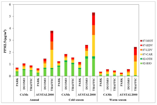
Figure 5.
Primary PM2.5 levels and source apportionment comparison between CAMx and AUSTAL2000 at the urban receptors (PARK, DUOMO, TRAFFIC) for LOCAL region emissions.
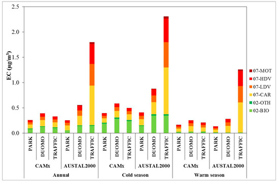
Figure 6.
EC levels and source apportionment comparison between CAMx and AUSTAL2000 at the urban receptors (PARK, DUOMO, TRAFFIC) for LOCAL region emissions.
CAMx limits in properly reproducing the impact of local sources are also confirmed by source apportionment results. Regardless for the period considered, CAMx provides very similar percentage contribution for source categories and sub-categories at the three receptors. Namely, for PPM2.5 traffic shares are 45.0–47.3%, 28.6–30.1%, and 72.6–73.7% respectively on annual, cold season, and warm season basis; corresponding figures for AUSTAL2000 are 52.2–82.3%, 36.7–68.9%, and 83.8–97%. Additionally, such a limited capability of reproducing the exposure to primary emission from road traffic is further highlighted by EC source apportionment, with CAMx traffic shares insensitive to receptors’ features (66%, 48%, and 86% on annual, cold season, and warm season basis) whereas AUSTAL2000 provides receptor-dependent shares (72.3–91.2%, 57.4–83.8%, and 92.2–98.7%).
In spite of the abovementioned limits of CAMx and notwithstanding the fact that two models are based on different approaches, their results are in rather good agreement at PARK receptor for both PPM2.5 (0.65 µg/m3 vs. 0.76 µg/m3 for the annual average and 1.17 µg/m3 vs. 1.32 µg/m3 and 0.28 µg/m3 vs. 0.40 µg/m3 for seasonal values) and especially for EC (both models predict 0.26 µg/m3 for EC annual average and 0.41 µg/m3 vs. 0.39 µg/m3, 0.14 µg/m3 vs. 0.17 µg/m3 for the seasonal values). Deviations between model outputs become larger and larger as the density of emission sources nearby the receptor increases (i.e., passing from PARK to DUOMO and to TRAFFIC receptor). Thus, CAMx results can be regarded as concentrations levels representative of receptors not directly exposed to local emissions but poorly representative of both residential areas and, most of all, of traffic exposed receptors, where the impact of local sources is missed.
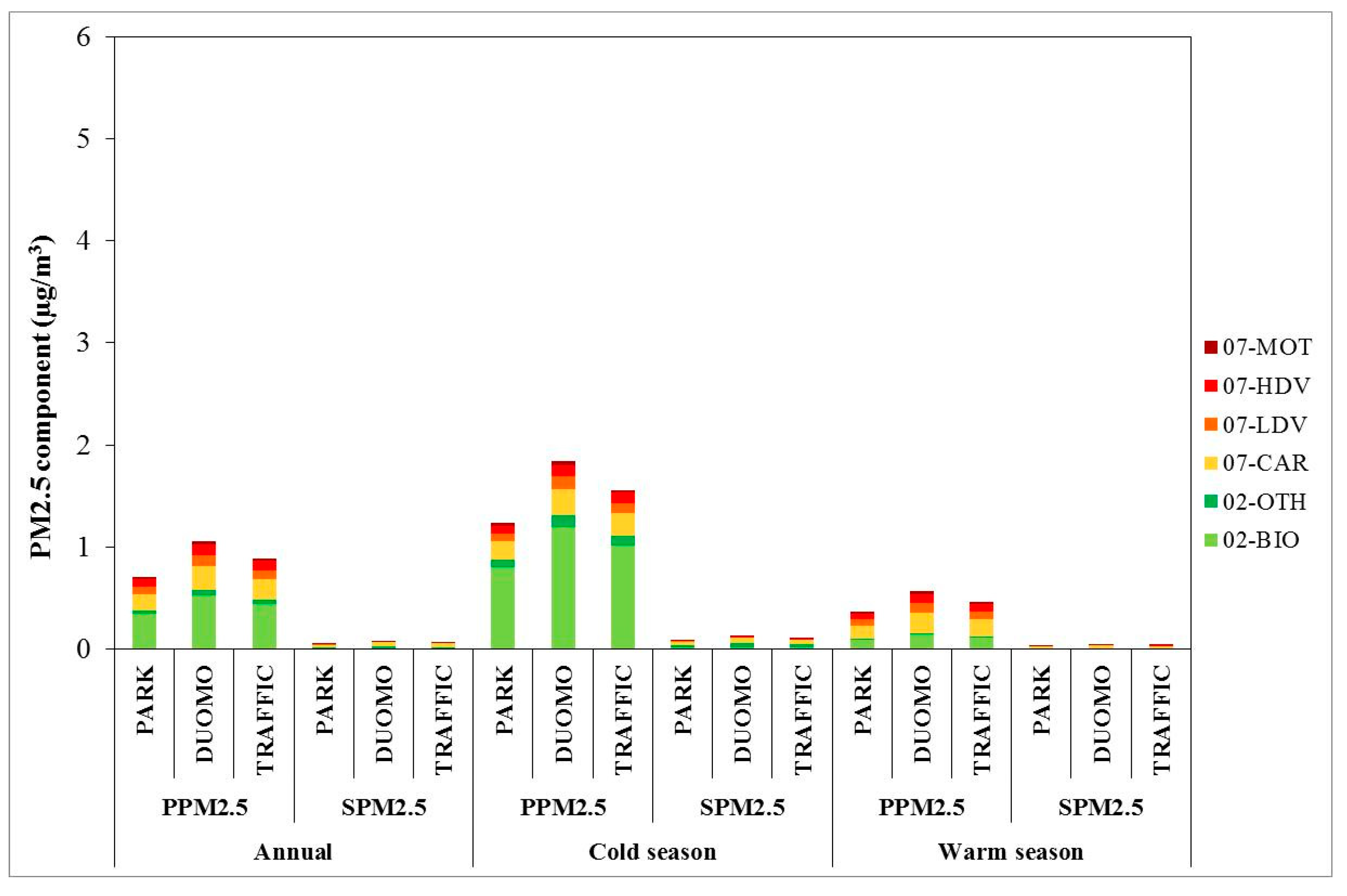
These outcomes are a direct consequence of the different emission spatialization degree within the LOCAL region adopted by the two models: AUSTAL2000 locates road traffic and domestic heating emissions in correspondence with the arches of the urban street network and of built areas; conversely, CAMx evenly distributes the emissions all over the region. Additionally, AUSTAL2000 really calculates concentrations at the receptors points, whereas CAMx determines the concentrations as a distance-based weighed average of the concentrations computed for the four grid cells nearest to the receptor. The drawback of AUSTAL2000 results is that they neglect the secondary PM generated by precursors emissions from the sources within the LOCAL region, that conversely CAMx is able to separately predict and apportion. However, as shown in Figure 7, the contribution of secondary PM to the total PM2.5 is very limited, roughly in the order of 6–7%. Thus, AUSTAL2000 enhanced capability of better reproducing the variability of the concentration levels at the local urban scale, according to receptors’ exposure to the emission sources, almost totally offsets the limitation of the neglected secondary PM formation processes.

Figure 7.
CAMx primary (PPM2.5) and secondary (SPM2.5) PM2.5 levels and source apportionment comparison at the urban receptors (PARK, DUOMO, TRAFFIC) for LOCAL region emissions.
3.3. HMS Output
Previous results demonstrate that AUSTAL2000 has a greater ability in reproducing the variability of concentration levels and source contributions at the local scale, thus supporting the setup of a Hybrid Modeling System (HMS) that combines the key features of CAMx and AUSTAL2000. At the receptors of the local scale urban domain the concentration predicted by the HMS is given by the sum of two terms: the former representing the contribution of sources located outside the urban domain, which accounts for PM secondary formation processes too, the latter representing the contribution of local sources, which neglects chemical processes but accounts for the receptors’ exposure to the emission sources. In practice, the spatially-variable and site-dependent contribution of local sources computed by AUSTAL2000 is superimposed to a common base produced by sources located elsewhere (CAMx Background). For the sake of accuracy, the secondary PM2.5 generated by the emissions from the LOCAL region estimated by CAMx was also accounted for within the LOCAL region contribution, in spite of its marginal contribution
3.3.1. PM2.5
HMS results for PM2.5 source apportionment are shown in Figure 8 that allows appreciating both source categories and emission regions contributions concurrently. Summary Tables for the estimated contributions are reported in Supplementary materials. As pointed out, the difference among the estimated concentration levels is driven by the contribution of the local sources, because the CAMx Background is the same at the three receptors, all located in the same cell of CAMx computational domain.
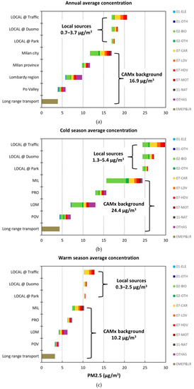
Figure 8.
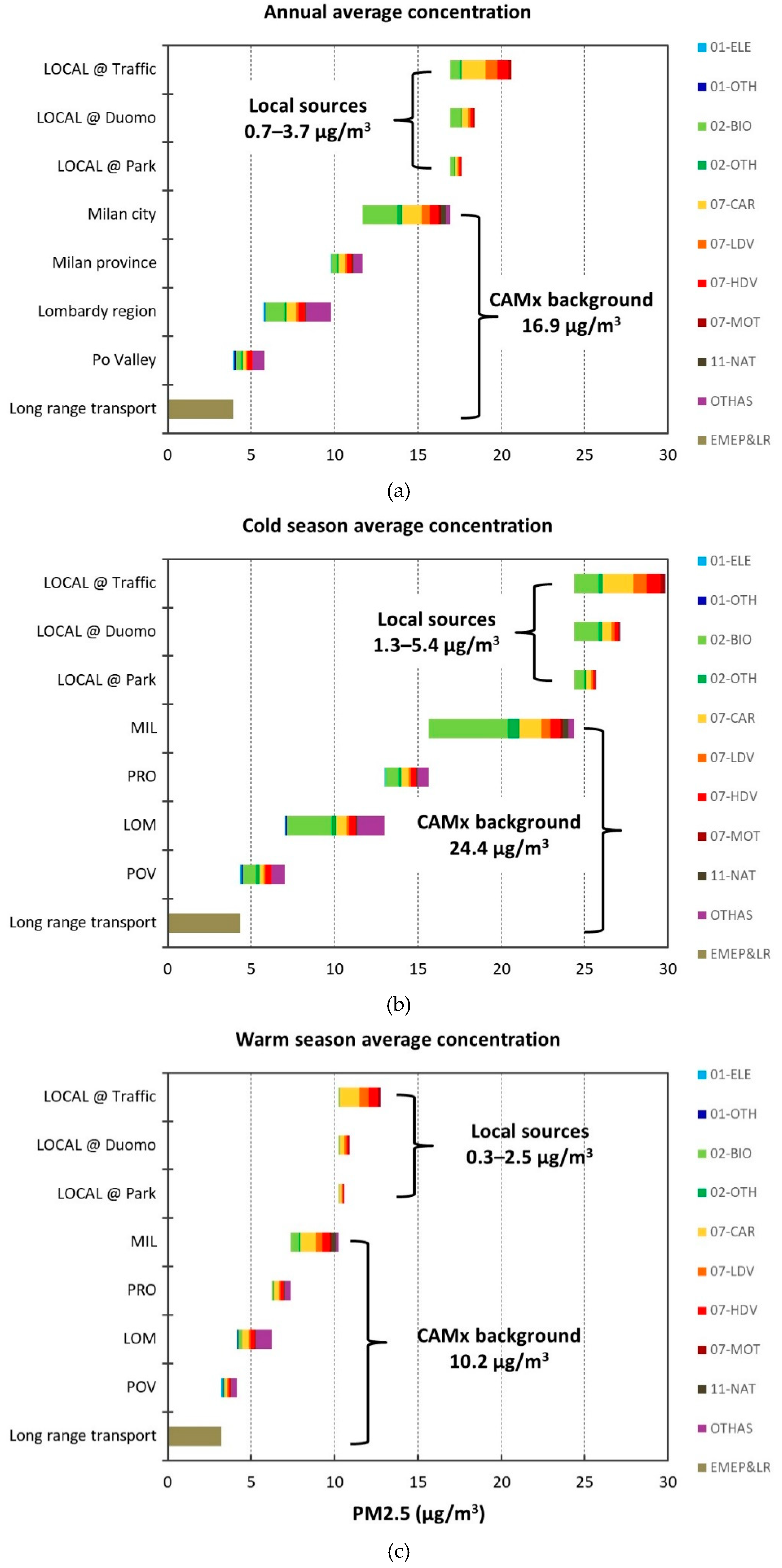
PM2.5 source apportionment by HMS for PARK, DUOMO, and TRAFFIC receptors for annual average (a), cold season average (b), warm season average concentration (c).
On annual basis (Figure 8a), the sources located outside the local domain (CAMx Background) are responsible for about 17 µg/m3, that is 96%, 92%, and 82% of the total estimated PM2.5 (17.6 µg/m3 at PARK, 18.4 µg/m3 at DUOMO, 20.6 µg/m3 at TRAFFIC); LOCAL contributions are in the 0.7–3.7 µg/m3 range. Among emission regions, MIL region is the first contributor (5.2 µg/m3, 25.5–29.9%), followed by LOM region (4.0 µg/m3, 19.5–22.9%) and by POV and PRO (both around 1.9 µg/m3, 9.0–10.7%); long range transport contributes with a 3rd-highest 3.9 µg/m3 (19.0–22.2%). In terms of emission categories, road traffic (5.2–7.8 µg/m3 range, 31.6–38.0%) slightly prevails on C&R combustion (4.8–5.2 µg/m3 range, 25.2–28.4%), both by far greater than the long-range transport and the other anthropogenic sources (OTHAS, 2.9 µg/m3, 14.3–16.8%). Figures for road traffic at the TRAFFIC receptor are higher than at the two other receptors both as concentration (7.8 µg/m3) and as percent share (39.0%) because of the additional contribution (3 µg/m3, 14.5% of total PM2.5 at TRAFFIC) from local traffic estimated by AUSTAL2000, sensitively greater than at DUOMO and, most of all, at PARK (0.38 µg/m3, 2.2% of total PM2.5 at PARK) as shown in Figure 7. Road traffic contribution mainly derives for ~40% from passenger cars emissions (07-CAR) and for ~30% from light- and heavy-duty vehicles; motorcycles are responsible for 2% only. C&R combustion almost entirely derives from biomass burning (02-BIO). When both emission regions and categories are considered, the features of the receptors come clearly to the light: at PARK and DUOMO road traffic (2.3 µg/m3) and biomass burning (2.1 µg/m3) from the MIL region are the first two contributors; conversely, at TRAFFIC road traffic from the LOCAL region (3.0 µg/m3) takes over. However, all these contributions are smaller than the one coming from long range transport (3.9 µg/m3), that accounts for about 20% of the total PM2.5.
Seasonal results (Figure 8b,c) point out the different activity of biomass burning, not only in the local region but also in all the other emission regions, sensitively affecting the total PM2.5 levels. Actually, in the cold season CAMx Background (24.4 µg/m3) is about 2.5 times as high as in the warm season (10.2 µg/m3) and LOCAL region contributions are from 2 to 4 times higher (cold season range 1.3–5.4 µg/m3 vs. warm season range 0.3–2.5 µg/m3). MIL region (8.7 µg/m3) and LOM region (6.0 µg/m3) are the two first contributors to PM2.5 levels: LOCAL region contribution is 3rd-highest at TRAFFIC (5.4 µg/m3) and at DUOMO (2.7 µg/m3), but is the lowest at PARK (1.3 µg/m3) where is doubled by both POV and PRO contributions (~2.6 µg/m3). Contribution from biomass burning is about 10 times higher than in the warm season (~10 µg/m3 vs. ~1 µg/m3), making this source the first contributor to PM2.5 at all the receptors, even at TRAFFIC site where it takes over road traffic (10.6 µg/m3 vs. 9.1 µg/m3). Overall, biomass burning accounts for 35.7–39.3% of total PM2.5, mostly deriving from the MIL and LOM region (45–49% and 25.7–28% of 02-BIO contribution, respectively). Biomass burning from the MIL (4.8 µg/m3) and LOM region (2.7 µg/m3) are the two top contributors in the joint breakdown by emission regions and categories, followed by OTHAS contribution from LOM region (2.9 µg/m3) at PARK and DUOMO and by passenger cars contribution (07-CAR, 1.8 µg/m3) from the LOCAL region at TRAFFIC receptor.
In the warm season the contributions from the 4 outermost regions prevails on that from the LOCAL region, still with MIL and LOM regions as top contributors (2.8 µg/m3 and 2.1 µg/m3 respectively); conversely, at TRAFFIC receptor road traffic emissions from the LOCAL region become the 2nd-most contributor (2.4 µg/m3). Almost missing the C&R combustion, road traffic is the first source of PM2.5, accounting for about 36% at PARK and DUOMO, but up to 46% (5.9 µg/m3) at TRAFFIC, due to the relevant contribution from the LOCAL region, followed by long range transport (25–30%) and OTHAS (15–17%). The primary role of road traffic is also confirmed by joint regions-categories breakdown: traffic emissions from the MIL region are responsible for a top 1.8 µg/m3 at PARK and DUOMO (17% of total PM2.5), whereas those from the LOCAL region are the 1st-contributor at TRAFFIC (2.5 µg/m3 of total PM2.5). Overall, traffic emissions from the entire Milan municipality (i.e., LOCAL + MIL region) determine 2.2 µg/m3 (PARK), 2.5 µg/m3 (DUOMO), and 4.3 µg/m3 (TRAFFIC), that is, respectively, 20%, 23%, and 34% of the total estimated PM2.5 at the three receptors.
3.3.2. EC
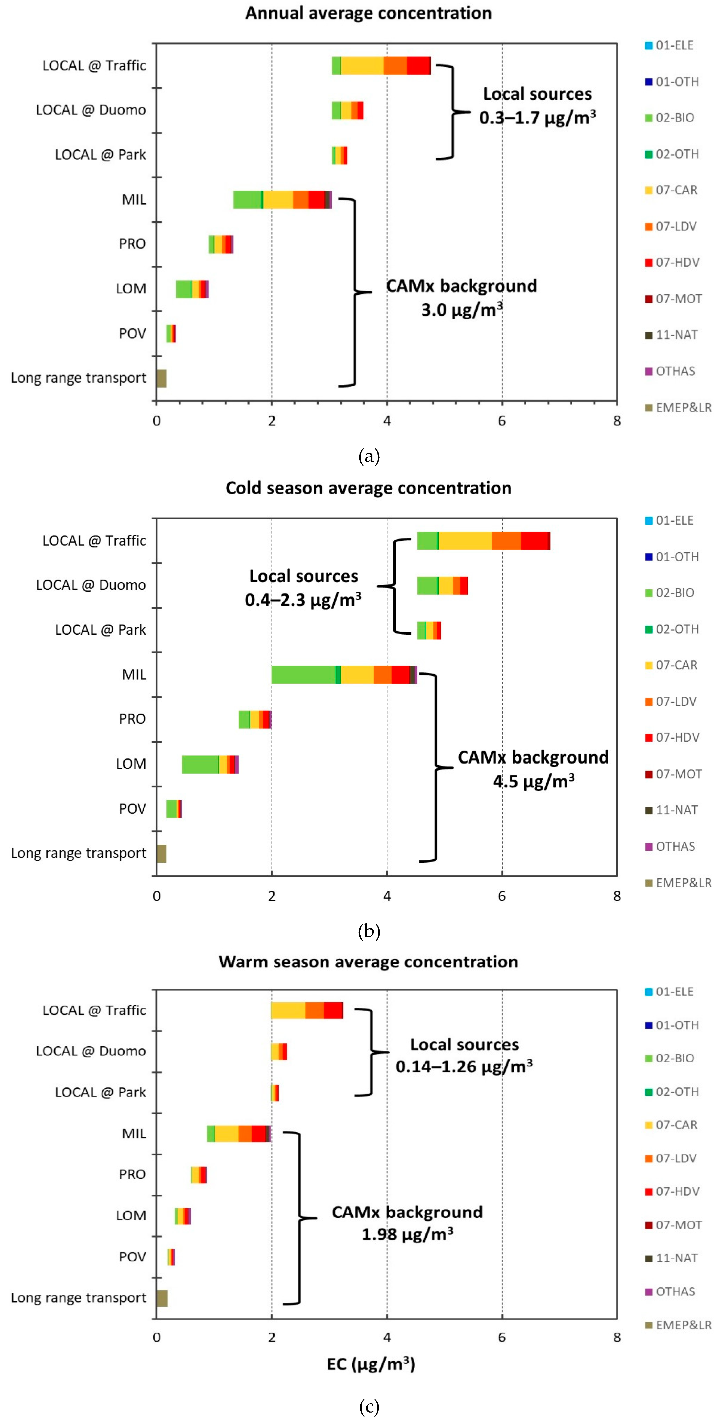
Estimated EC levels and related source and region apportionment are presented in the panels of Figure 9. As annual average, EC concentration is in the 3.3–4.7 µg/m3 range, strongly receptor-dependent because of the strong variation in the LOCAL region contributions (0.3–1.7 µg/m3) in addition to the CAMx Background of 3.0 µg/m3 (Figure 9a). Such receptor-dependency is due to the great difference among local road traffic contributions, ranging between a minimum of 0.2 µg/m3 at PARK up to a maximum of 1.6 µg/m3 at TRAFFIC receptor. Overall, road traffic emissions are responsible for about 57% of EC at PARK and DUOMO (~1.9 µg/m3) and of 68% (3.2 µg/m3) at TRAFFIC, but at the two former receptors the traffic contribution originates from the MIL region traffic (30–32% of total EC) whereas at the latter receptor LOCAL region (33%) prevails on MIL region contribution (23%). The contribution of C&R combustion (~1.1 µg/m3) is in the order of 31% at PARK and DUOMO and down to 23% at TRAFFIC, with the MIL region responsible for about half of these contributions.
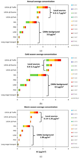
Figure 9.
EC source apportionment by HMS for PARK, DUOMO and TRAFFIC receptors for annual average (a), cold season average (b), warm season average concentration (c).
The comparison between seasonal results (Figure 9b,c) highlights the wintertime contribution of biomass burning: at PARK and DUOMO biomass combustion (~2.5 µg/m3, 48%) slightly prevails on road traffic provide almost the same contribution (2.2 µg/m3, 43%); at TRAFFIC, the latter source prevails (3.8 µg/m3 vs. 2.6 µg/m3, that is 56% vs. 38% of total EC). Conversely, in summertime biomass combustion displays a much lower contribution (0.25 µg/m3), almost entirely deriving from sources outside the LOCAL region, and at all receptors road traffic is, by far, the first contributor overall (1.5–2.6 µg/m3, that is 70–80% of EC). As far as traffic contribution is concerned, on both in the cold and warm season the LOCAL region contribution prevails on the MIL region one at the TRAFFIC receptor (1.9 µg/m3 vs. 1.2 µg/m3 and 1.2 µg/m3 vs. 0.9 µg/m3, respectively) contrary to the two other receptors, and especially at PARK, where LOCAL region (0.26 µg/m3 and 0.12 µg/m3) is by far exceeded by the MIL region contribution.
4. Conclusions
A hybrid modeling system (HMS), which couples the Eulerian chemical and transport model CAMx with the local-scale Lagrangian model AUSTAL2000, was set up for air quality assessment and source apportionment in urban areas. In the HMS approach, estimated concentration levels come from the superposition of the background contribution of emission sources located outside the local-scale urban domain, assessed by the Eulerian component, and of the contribution of sources within this latter domain, assessed by the Lagrangian component. In comparison with the Eulerian model, the Lagrangian component relies on a better spatial distribution of emission sources within its computational domain, unevenly distributed because of the road network layout (for traffic emissions) and of the built environment structure (for space heating). Such refinement in the spatialization of local emissions allows the HMS to reproduce more realistically the variability of concentration levels among urban receptors (within the local-scale domain), according to their actual exposure to local sources. In this work, the enhanced performance of the HMS has been assessed for three selected receptors, located in a relatively small area of Milan city center and representative of different exposure to emission sources (PARK receptor: urban background; TRAFFIC receptor: heavy urban traffic; DUOMO receptor: urban traffic, commercial and residential emissions). However, this promising result is someway limited by the few receptors considered and the limited extension of the modelled area by the Lagrangian component. Therefore, these first outcomes need to be further confirmed by future work where, extending the computational domain of the Lagrangian component, a larger number of receptors (e.g., residential areas outside city center, city outskirts, main access roads to the city) can be considered, in order to account for the complex spatial variability of air pollution within the whole urban area. Future work could also include the development of alternative local scale modeling layers, based either on Lagrangian modeling approach, such as puff models, as well as on geostatistical-based methods, both allowing the extensions of the analysis to larger portions of the urban area.
For the presented case-study, the HMS results in almost a 6× factor between PM2.5 annual average at the traffic exposed receptor and at the background receptor in a green area, whereas the Eulerian model, missing the impact of local traffic at the former receptor, predicts only a 26% difference. In practice, the outcome of the Eulerian model at the local scale is only representative of a background level, similar to HMS outcome for the green area receptor, but fails to reproduce concentration gradients and hot-spots, driven by local sources’ emissions.
The HMS shows the potential for source apportionment evaluations based on both emission source categories, emission regions (i.e., user-defined areas where sources ae located), and on the combination of categories with regions. This feature enables to assess the overall contribution to ambient concentration levels of the different sources, but also to split the contribution based on geographical location of the sources, that may significantly vary in relation to the receptors’ exposure to local sources. In our case-study, at the two receptors less exposed to vehicular emissions, domestic heating and road traffic almost equally contribute to PM2.5 annual average concentration (30%), Milan’s urban area is the top contributor among emission regions (29.6%), and road traffic from Milan’s urban area is the top contributor (13%) when both emission categories and regions are considered. At the traffic-exposed receptor, road traffic is the top contributor (38%), the Milan region is still the main origin for PM2.5, but with a lower share (25%), and local road traffic is the first contributor (14.5%) in the joint emission categories and regions analysis. The different features of the receptors, namely their exposure to local traffic emissions, are confirmed by PM2.5 source apportionment results on seasonal basis and for elemental carbon too. Thus, the enhanced reproduction of the impact of local sources ensured by the Lagrangian component of the HMS allows to better assess and properly put in context sources’ contributions. Additionally, the joint apportionment by categories and regions provides a piece of information that receptor models cannot provide, as their outcome is limited to sources’ identification and overall contribution estimation.
This peculiar output of the HMS is particularly useful for scenario evaluations in the framework of air quality remediation and management plans, because it allows the prediction of the outcome of interventions and policies at different spatial scales. Implementation of a small low-emission-zone can affect traffic emissions at the very local scale, whereas the adoption of a congestion/pollution charging scheme, or the ban for diesel vehicles prospected for some European large cities in the near future, has a wider impact, affecting emissions at the urban scale. From the space heating standpoint, implementation/enlargement of district heating at the municipality level may affect local/urban scale emissions, whereas policies on fuels, like limitations or bans in biomass use for domestic heating, usually act on larger administrative areas, therefore potentially affecting emissions even up to the regional scale.
Supplementary Materials
The following are available online at https://www.mdpi.com/2073-4433/11/10/1078/s1, Table S1. Lambert Conformal coordinates for Po valley and Milan metropolitan area nested domains in WRF and CAMx model. Table S2. Emission categories defined considered for source apportionment. Table S3. Annual and seasonal average concentrations of PM2.5 and relative contributions by source regions. Table S4. Contributions (µg/m3) by source regions to the annual PM2.5 concentrations. Figure S1. Time series of the box and whisker plots for the distribution of the observed (black/grey) and computed (red/orange) daily mean values of mixing ratio, temperature and wind speed over Milan metropolitan area for 2010. Bars show the interquartile range (IR), lines the median values, dashed vertical bars (25th – 1.5 · IR) and the (75th + 1.5 · IR) value. Values for the 25th, 50th, 75th, and 95th quantiles of the whole yearly time series are reported too. (Pepe et al., 2016). Figure S2. Wind rose for calendar year 2010 at Milano Linate airport (5 km crow-fly distance East from Milano city center). Figure S3. Emission regions within Po Valley (top panel, 5 km grid step) and Milan metropolitan area (bottom panel, 1.7 km grid step) computational domains. Figure S4. Google street views of the surroundings of DUOMO receptor. Figure S5. Google street views of the surroundings of PARK receptor. Figure S6. Google street views of the surroundings of TRAFFIC receptor.
Author Contributions
Conceptualization and methodology: G.P.; Software and Modelling simulations: N.P., A.B., A.T., G.M.R.; Formal Analysis: G.L.; Data Curation: N.P. and G.L.; Writing—Original Draft Preparation: G.L.; Writing—Review & Editing, G.L. and G.P. All authors have read and agreed to the published version of the manuscript.
Funding
This research received no external funding.
Acknowledgments
This work has been financed by the Research Fund for the Italian Electrical System under the Contract Agreement between RSE S.p.A. and the Ministry of Economic Development—General Directorate for Nuclear Energy, Renewable Energy and Energy Efficiency in compliance with the Decree of March 8, 2006.
Conflicts of Interest
The authors declare no conflict of interest.
References
- Forouzanfar, M.H.; Afshin, A.; Alexander, L.T.; Anderson, H.R.; Bhutta, Z.A.; Biryukov, S.; Brauer, M.; Burnett, R.; Cercy, K.; Charlson, F.J.; et al. Global, regional, and national comparative risk assessment of 79 behavioural, environmental and occupational, and metabolic risks or clusters of risks, 1990–2015: A systematic analysis for the Global Burden of Disease Study 2015. Lancet 2016, 388, 1659–1724. [Google Scholar] [CrossRef]
- World Health Organization (WHO). Ambient Air Pollution: A Global Assessment of Exposure and Burden of Disease; WHO: Geneva, Switzerland, 2016. [Google Scholar]
- Kelly, F.J.; Fussel, J.C. Air pollution and public health: Emerging hazards and improved understanding of risk. Environ. Geochem. Health 2015, 37, 631–649. [Google Scholar] [CrossRef] [PubMed]
- World Health Organization (WHO). Regional Office for Europe, 2013. Review of Evidence on Health Aspects of Air Pollution—REVIHAAP Project, Technical Report; WHO: Geneva, Switzerland, 2013. [Google Scholar]
- Lelieveld, J.; Pozzer, A.; Pöschl, U.; Fnais, M.; Haines, A.; Münzel, T. Loss of life expectancy from air pollution compared to other risk factors: A worldwide perspective. Cardiovasc. Res. 2020, 116, 1910–1917. [Google Scholar] [CrossRef] [PubMed]
- Duyzer, J.; van der Hout, D.; Zandveld, P.; van Ratigen, S. Representativeness of air quality monitoring networks. Atmos. Environ. 2015, 104, 88–101. [Google Scholar] [CrossRef]
- Ciarelli, G.; Aksoyoglu, S.; El Haddad, I.; Bruns, E.A.; Crippa, M.; Poulain, L.; Äijäkä, M.; Carbone, S.; Freney, E.; O’Dowd, C.; et al. Modelling winter organic aerosol at the European scale with CAMx: Evaluation and source apportionment with a VBS parameterization based on novel wood burning smog chamber experiments. Atmos. Chem. Phys. 2017, 17, 7653–7669. [Google Scholar] [CrossRef]
- Squizzato, S.; Cazzaro, M.; Innocente, E.; Visin, F.; Hopke, P.; Rampazzo, G. Urban air quality in a mid-size city – PM2.5 composition, sources and identification of impact areas: From local to long range contributions. Atmos. Res. 2017, 186, 51–62. [Google Scholar] [CrossRef]
- Pirovano, G.; Colombi, C.; Balzarini, A.; Riva, G.M.; Gianelle, V.; Lonati, G. PM2.5 source apportionment in Lombardy (Italy): Comparison of receptor and chemistry transport modelling results. Atmos. Environ. 2015, 106, 56–70. [Google Scholar] [CrossRef]
- European Union. Directive 2008/50/EC of the European Parliament and of the Council of 21 May 2008 on ambient air quality and cleaner air for Europe. Off. J. Eur. Union 2008, 152, 1–44. [Google Scholar]
- Zou, B.; Wilson, J.G.; Zhan, F.B.; Zeng, Y. Air pollution exposure assessment methods utilized in epidemiological studies. J. Environ. Monitor. 2009, 11, 475–490. [Google Scholar] [CrossRef]
- Lenschow, P.; Abraham, H.-J.; Kutzner, K.; Lutz, M.; Preuß, J.-D.; Reichenbächer, W. Some ideas about the sources of PM10. Atmos. Environ. 2001, 35, S23–S33. [Google Scholar] [CrossRef]
- Vardoulakis, S.; Fisher, B.E.; Pericleous, K.; Gonzalez-Flesca, N. Modelling air quality in street canyons: A review. Atmos. Environ. 2003, 37, 155–182. [Google Scholar] [CrossRef]
- Guevara, M.; Jorba, O.; Tena, C.; van der Gon, H.D.; Kuenen, J.; Elguindi-Solmon, N.; Darras, S.; Granier, C.; García-Pando, C.P. CAMS-TEMPO: Global and European emission temporal profile maps for atmospheric chemistry modelling. Earth Syst. Sci. Data Discuss. 2020. [Google Scholar] [CrossRef]
- López-Aparicio, S.; Guevara, M.; Thunis, P.; Cuvelier, K.; Tarrasón, L. Assessment of discrepancies between bottom-up and regional emission inventories in Norwegian urban areas. Atmos. Environ. 2017, 154, 285–296. [Google Scholar] [CrossRef]
- van der Gon, H.A.; Bergström, R.; Fountoukis, C.; Johansson, C.; Pandis, S.N.; Simpson, D.; Visschedijk, A.J.H. Particulate emissions from residential wood combustion in Europe - revised estimates and an evaluation. Atmos. Chem. Phys. 2015, 15, 6503–6519. [Google Scholar] [CrossRef]
- Guevara, M.; Pay, M.T.; Martínez, F.; Soret, A.; Denier van der Gon, H.A.C.; Baldasano, J.M. Inter-comparison between HERMESv2.0 and TNO-MACC-II emission data using the CALIOPE air quality system (Spain). Atmos. Environ. 2014, 98, 134–145. [Google Scholar] [CrossRef]
- Bessagnet, B.; Pirovano, G.; Mircea, M.; Cuvelier, C.; Aulinger, A.; Calori, G.; Ciarelli, G.; Manders, A.; Stern, R.; Tsyro, S.; et al. Presentation of the EURODELTA III intercomparison exercise – evaluation of the chemistry transport models’ performance on criteria pollutants and joint analysis with meteorology. Atmos. Chem. Phys. 2016, 16, 12667–12701. [Google Scholar] [CrossRef]
- Pernigotti, D.; Thunis, P.; Cuvelier, C.; Georgieva, E.; Gsella, A.; De Meij, A.; Pirovano, G.; Balzarini, A.; Riva, G.M.; Carnevale, C.; et al. POMI: A model inter-comparison exercise over the Po valley. Air Qual. Atmos. Health 2013, 6, 701–715. [Google Scholar] [CrossRef]
- Cowie, C.T.; Garden, F.; Jegasothy, E.; Knibbs, L.D.; Hanigan, I.; Morley, D.; Hansell, A.; Hoek, G.; Marks, G.B. Comparison of model estimates from an intra-city land use regression model with a national satellite-LUR and a regional Bayesian Maximum Entropy model, in estimating NO2 for a birth cohort in Sydney, Australia. Environ. Res. 2019, 174, 24–34. [Google Scholar] [CrossRef]
- He, B.; Heal, M.R.; Reis, S. Land-Use Regression Modelling of Intra-Urban Air Pollution Variation in China: Current Status and Future Needs. Atmosphere 2018, 9, 134. [Google Scholar] [CrossRef]
- Hennig, F.; Sugiri, D.; Tzivian, L.; Fuks KMoebus, S.; Jöckel, K.-H.; Vienneau, D.; Kuhlbusch, T.; de Hoogh, K.; Memmesheimer, M.; Jakobs, H.; et al. Comparison of Land-Use Regression modeling with dispersion and chemistry transport modeling to assign air pollution concentrations within the Ruhr area. Atmosphere 2016, 7, 48. [Google Scholar] [CrossRef]
- Wang, M.; Sampson, P.D.; Hu, J.; Kleeman, M.; Keller, J.P.; Olives, C.; Szpiro, A.A.; Vedal, S.; Kaufman, J.D. Combining Land-Use regression and chemical transport modeling in a spatiotemporal geostatistical model for ozone and PM2.5. Environ. Sci. Technol. 2016, 50, 5111–5118. [Google Scholar] [CrossRef] [PubMed]
- Akita, Y.; Baldasano, J.M.; Beelen, R.; Cirach, M.; de Hoogh, K.; Hoek, G.; Nieuwenhuijsen, M.; Serre, M.L.; de Nazelle, A. Large scale air pollution estimation method combining land use regression and chemical transport modeling in a geostatistical framework. Environ. Sci. Technol. 2014, 48, 4452–4459. [Google Scholar] [CrossRef] [PubMed]
- Pepe, N.; Pirovano, G.; Balzarini, A.; Toppetti, A.; Riva, G.M.; Amato, F.; Lonati, G. Enhanced CAMx source apportionment analysis at an urban receptor in Milan based on source categories and emission regions. Atmos. Environ. 2019, X2, 100020. [Google Scholar] [CrossRef]
- Pepe, N.; Pirovano, G.; Lonati, G.; Balzarini, A.; Toppetti, A.; Riva, G.M.; Bedogni, M. Development and application of a high resolution hybrid modelling system for the evaluation of urban air quality. Atmos. Environ. 2016, 141, 297–311. [Google Scholar] [CrossRef]
- Berchet, A.; Zink, K.; Arfire, A.; Marjovi, A.; Martinoli, A.; Emmenegger, L.; Brunner, D. High-resolution air pollution modeling for urban environments in support of dense multi-platform networks. Geophys. Res. Abstr. 2015, 17, EGU2015-11161. [Google Scholar]
- Ghermandi, G.; Fabbi, S.; Bigi, A.; Veratti, G.; Despini, F.; Teggi, S.; Barbieri, C.; Torreggiani, L. Impact assessment of vehicular exhaust emissions by microscale simulation using automatic traffic flow measurements. Atmos. Pollut. Res. 2019. [Google Scholar] [CrossRef]
- Skamarock, W.C.; Klemp, J.B.; Dudhia, J.; Gill, D.O.; Barker, D.M.; Duda, M.G.; Huang, X.-Y.; Wang, W.; Powers, J.G. A Description of the Advanced Research WRF Version 3, NCAR Technical Note NCAR/TN-475+STR; University Corporation for Atmospheric Research: Boulder, CO, USA, 2008. [Google Scholar]
- ENVIRON. CAMx (Comprehensive Air Quality Model with extensions) User’s Guide Version 6.3; Environ International Corporation: Novato, CA, USA, 2016. [Google Scholar]
- Janicke Consulting. AUSTAL2000 Program Documentation of Version 2.6 2014-02-24; Federal Environmental Agency (UBA): Dessau-Roßlau, Germany, 2014.
- University of North Carolina at Chapel Hill (UNC). SMOKE v3.5 User’s Manual. 2013. Available online: https://www.cmascenter.org/smoke/documentation/3.5/manual_smokev35.pdf (accessed on 9 October 2020).
- European Land Use Atlas Data. Available online: http://www.eea.europa.eu/data-and-maps/data/urban-atlas (accessed on 9 October 2020).
- European Monitoring and Evaluation Programme data (EMEP). Available online: https://www.ceip.at/webdab-emission-database (accessed on 9 October 2020).
- Italian National Inventory Data. Available online: http://www.sinanet.isprambiente.it/it/sia-ispra/inventaria/disaggregazione-dellinventario-nazionale-2015/view (accessed on 9 October 2020).
- ARPA Lombardia. INEMAR, Inventario Emissioni in Atmosfera: Emissioni in Regione Lombardia Nell’anno 2012—Revisione Pubblica. ARPA Lombardia Settore Monitoraggi Ambientali. Available online: https://www.inemar.eu/xwiki/bin/view/InemarDatiWeb/Aggiornamenti+dell%27inventario+2012 (accessed on 9 October 2020).
- Yarwood, G.; Morris, R.E.; Wilson, G.M. Particulate matter source apportionment technology (PSAT) in the CAMx photochemical grid model. In Proceedings of the 27th NATO/CCMS International Technical Meeting on Air Pollution Modeling and Application, Banff, AB, Canada, 24–29 October 2004. [Google Scholar]
- Janssen, N.A.H.; Gerlofs-Nijland, M.E.; Lanki, T.; Salonen, R.O.; Cassee, F.; Hoek, G.; Fischer, P.; Brunekreef, B.; Krzyzanowski, M. Health Effects of Black Carbon; WHO: Copenhagen, Denmark, 2012. [Google Scholar]
- Amann, M.; Bertok, I.; Borken-Kleefeld, J.; Cofala, J.; Heyes, C.; Höglund-Isaksson, L.; Klimont, Z.; Nguyen, B.; Posch, M.; Rafaj, P.; et al. Cost-effective control of air quality and greenhouse gases in Europe: Modeling and policy applications. Environ. Model. Softw. 2011, 26, 1489–1501. [Google Scholar] [CrossRef]
© 2020 by the authors. Licensee MDPI, Basel, Switzerland. This article is an open access article distributed under the terms and conditions of the Creative Commons Attribution (CC BY) license (http://creativecommons.org/licenses/by/4.0/).


