COSMO-CLM Performance and Projection of Daily and Hourly Temperatures Reaching 50 °C or Higher in Southern Iraq

Abstract

Fortunately, extreme temperatures reaching 50 °C are not common on our planet. The capability of the consortium for small-scale modelling regional climate model (COSMO-CLM), with 0.44° resolution, to project future trends of an extremely hot environment with direct model output (DMO) is questioned. The temperature distribution of COSMO-CLM output driven by reanalysis and RCP4.5 scenario in southern Iraq was remarkably good, with a slight temperature overestimation, compared to the overlapping observations from Basra airport. An attempt to enhance the DMO with a statistical downscaling method did not improve the results. The COSMO-CLM projection indicates that a very sharp increase in the number of consecutive hours and days with the temperature reaching 50 °C or higher will occur. During 1951–1980, consecutive hours and days reaching 50 °C were rare events. By the end of the century, the projected climate in southern Iraq contains up to 13 consecutive hours and 21 consecutive days reaching 50 °C or higher. As the average projected temperature will increase by ~2 °C compared to the recent climate, new records may be expected. However, the major climate change feature is the increase in consecutive hours and days of very high temperatures. These findings require adaptation measures to support future habitation of the region.

1. Introduction

The earth’s climate evolution in the Mid-Holocene, such as the end of the green Sahara episode, forced human adaptation and gave rise to new civilizations [1]. Southern Iraq is the pre-historically region of southern Mesopotamia, which is often referred to as one of the cradles of civilizations. A place where mankind first began to read, write, create laws, and live in cities under an organized government at the Ubaid (6500–3800 BC) and Uruk periods (4000 to 3100 BC) (Figure 1). The changes in climate are further associated with the rises and collapses of empires throughout human history [2,3]. The biblical Garden of Eden paradise is also associated with southern Iraq.

The current climate in southern Iraq already contains days with temperatures higher than 50 °C [4]. Exposure of humans and other mammals to high temperatures for extended periods would be at risk for life-threatening hyperthermia and dehydration [5]. High temperatures increase the risk of various health problems such as kidney stones [6,7] and low birth weight [8]. Global warming projections indicate a reduction of agricultural yields [9]. Extreme heat significantly reduced cereal production [10] and there is evidence that temperatures of 50 °C are lethal for seeds of all species [11]. If due to global warming, temperatures will further increase, there is a set of external climatic conditions beyond which adequate physiological cooling cannot occur and areas as southern Iraq may reach the limitations to thermoregulation and acclimatization for human adaptation [12]. It might imply intolerable conditions and call into question the region’s suitability for human habitation [13]. Using an ensemble of regional climate models (RCM) project that around the Arabian Gulf extremes conditions may exceed a threshold for human adaptability [14].

Historical mean monthly data from Basra available from 1923 to 2013 indicates an increase in temperature and reduced precipitation [15]. For the years 1965–2015, the temperature in Iraq is increasing 2 to 7 times faster than the global temperature rise [16].

Sensitivity analysis with the COSMO-CLM over the Middle East and North Africa (MENA) domain of COordinated Regional Downscaling EXperiment (CORDEX) indicated that the mean absolute error value for temperature is about 1.2 °C [17]. Climate change projections for the MENA domain with COSMO-CLM with 0.44° and 0.22° resolution show significant warming expected over the whole area considered at the end of the 21st century, along with a reduction in precipitation [18]. Over the eastern Mediterranean, the same model driven by ERA-Interim reanalysis has demonstrated the capability to reproduce the climate characteristics, including extreme values. A general overestimation of maximum temperature indices is reported [19]. Salman et al. [20] using four general circulation models (GCMs) showed that the maximum temperatures in Iraq will increase in the range of 1.7–2.9 °C, 1.8–4.4 °C, 1.5–4.9 °C, and 1.7–6.8 °C under radiative forcing pathway RCP2.6, RCP4.5, RCP6.0, and RCP8.5 scenarios, respectively during 2070–2099.

A heat wave is defined when a specific temperature threshold is exceeded, thus allowing analysis of heat waves duration and frequency. Future behavior of heat waves in the global parallel climate model (PCM) indicates more intense, more frequent, and longer-lasting heat waves in the 21st century [21].The study goal is to examine if the direct model output (DMO) from the COSMO-CLM RCM, with 0.44° resolution, is accurate enough to give projections of the consecutive hours and of days with the temperature reaching 50 °C or higher, in southern Iraq.

Boundary conditions originating from the host GCM and the RCM errors, which result from approximations in the dynamics formulation, physical parameterizations, or numerical schemes [22] impose many sources of uncertainty for climate projections. Model output presents an area average of the model grid box as compared to point measurement of a meteorological station. However, if a threshold-based index as reaching 50 °C or higher is analyzed the point measurement and the simulated values most have the same distribution. Otherwise, the analysis will be erroneous.

In many cases, the simulated distribution is not similar to the point observation distribution. Many statistical downscaling (SD) techniques are available to amend the simulated distributions to fit the observations. These techniques downscale the large-scale model output to a point measurement [21,23,24]. Quantile mapping (QM) is a common SD method for model bias correction [25,26]. Another goal of this research is to evaluate the benefit of the CDF-t SD method, which is an improvement of the QM method [27].

2. Materials and Methods

2.1. Climate Model and Simulations

The RCM COSMO-CLM [28] with an hourly output was used to project the change in the daily and hourly frequency of temperatures reaching 50 °C or higher in the Basra area (Figure 1). The simulations were performed at the Israel Meteorological Service with a horizontal resolution of 0.44 and 40 model levels at the CORDEX [29] MENA domain. The domain extends from latitude 7° S to 45° N and from longitude 27° W to 76° E. Southern Iraq is located in the center of the domain and far from the boundaries relaxation zone.

The first simulation was driven by the ERA-Interim reanalysis [30] for the years 1979–2014, to tune the model parameters and verify the model’s ability to follow the day-by-day temperature and precipitation. The second simulation performed between the years 1950 to 2100 was driven by the MPI-M Earth System Model ECHAM data, which is part of the Coupled Model Intercomparison Project phase 5 (CMIP5) experiment [31]. The projection from 2005 to 2100 assumed the radiative forcing pathway (RCP) which leads to radiative forcing of 4.5 W/m² by the year 2100 (RCP4.5). The equivalent CO₂ concentrations corresponding to 4.5 W/m² forcing, is approximately 630 ppm [32].

The selection of the intermediate scenario RCP4.5, which resides between the stringent mitigation scenario (RCP2.6) and the very high greenhouse gas emissions scenario (RCP8.5), will impose moderate results.

2.2. Observations

Meteorological Terminal Air Report (METAR) hourly temperature observations from Basra airport (Figure 1) are available from 2 July 2012 to 31 December 2019 for model verification. METAR observations of temperatures are given as integer values and are made manually with many typos and missing data. Therefore, METAR observations from Abadan airport, located 57 km to the southeast of Basra, were used for data quality assurance and filling missing values on hot days.

2.3. Statistical Downscaling (SD)

To produce a more accurate and reliable local projection of temperature, the cumulative distribution function transform (CDF-t) statistical downscaling method was tested. CDF-t method for bias correction [27] finds a transformation that maps the model CDF of the climate temperature in the historical period to the observed CDF of Basra measurements and then applies that same mapping to the model’s future CDF [23,27]. The SD computations have been made through the “CDF-t” R package (freely available on www.r-project.org) [33].

3. Results

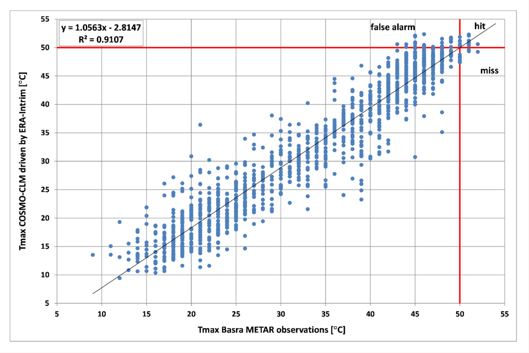
3.1. COSMO-CLM Driven by the ERA-Interim Reanalysis

Figure 2 presents the day by day maximum temperature (Tmax) simulated by the COSMO-CLM driven by the ERA-Interim reanalysis as a function of Tmax observed at Basra airport. The overlapping period contains 3.5 years between mid-2011 to the end of 2014, where the observed average was 33.25 ± 0.61 °C compared to an average of 32.30 ± 0.67 °C obtained by the COSMO-CLM simulation. The correlation between the observed and simulated Tmax is 0.91 and the slope of the regression line is 1.056. If accounting only for the summer months from May to September (MJJAS) the correlation reduces to 0.57.

For 14 events both daily Tmax for the COSMO-CLM and the observations reached 50 °C or higher (hits). For 23 days, the simulated Tmax was above 50 °C but the observed did not reach 50 °C (false alarm). For 11 days, the simulation missed a Tmax of 50 °C or higher (

Table 1. Contingency table for daily Tmax reaching 50 °C or higher.

	Tmax ≥ 50 °C Observers	Tmax ≥ 50 °C Not Observed
Tmax ≥ 50 °C simulated	14 (hit)	23 (FA)
Tmax ≥ 50 °C not simulated	11(miss)	1167 (TN)

and Figure 2). The critical success index (CSI), which is the ratio between the hits and all the other cases except the true negative (TN) cases, is 0.289. Respectively, a positive bias frequency, which is equal to the total number of events forecasts divided by the total number of events observed, has a value of 1.48. These results indicate that the model is definitely capable of simulating temperatures above 50 °C, albeit with a tendency to over-forecast.

3.2. Daily and Hourly High Temperatures Frequency Projections

The COSMO-CLM simulations include a history run from 1950 to 2005 and a projected period from 2005 to 2100, assuming RCP4.5. There are eight full years (2012–2019) with overlapping between observations and simulated data, which are used to compare the COSMO-CLM simulated climate and the observed climate. Definition of four daily and hourly high temperatures indices for the daytime (7:00–18:00 UTC) during the five summer months from May to September (MJJAS) are given:

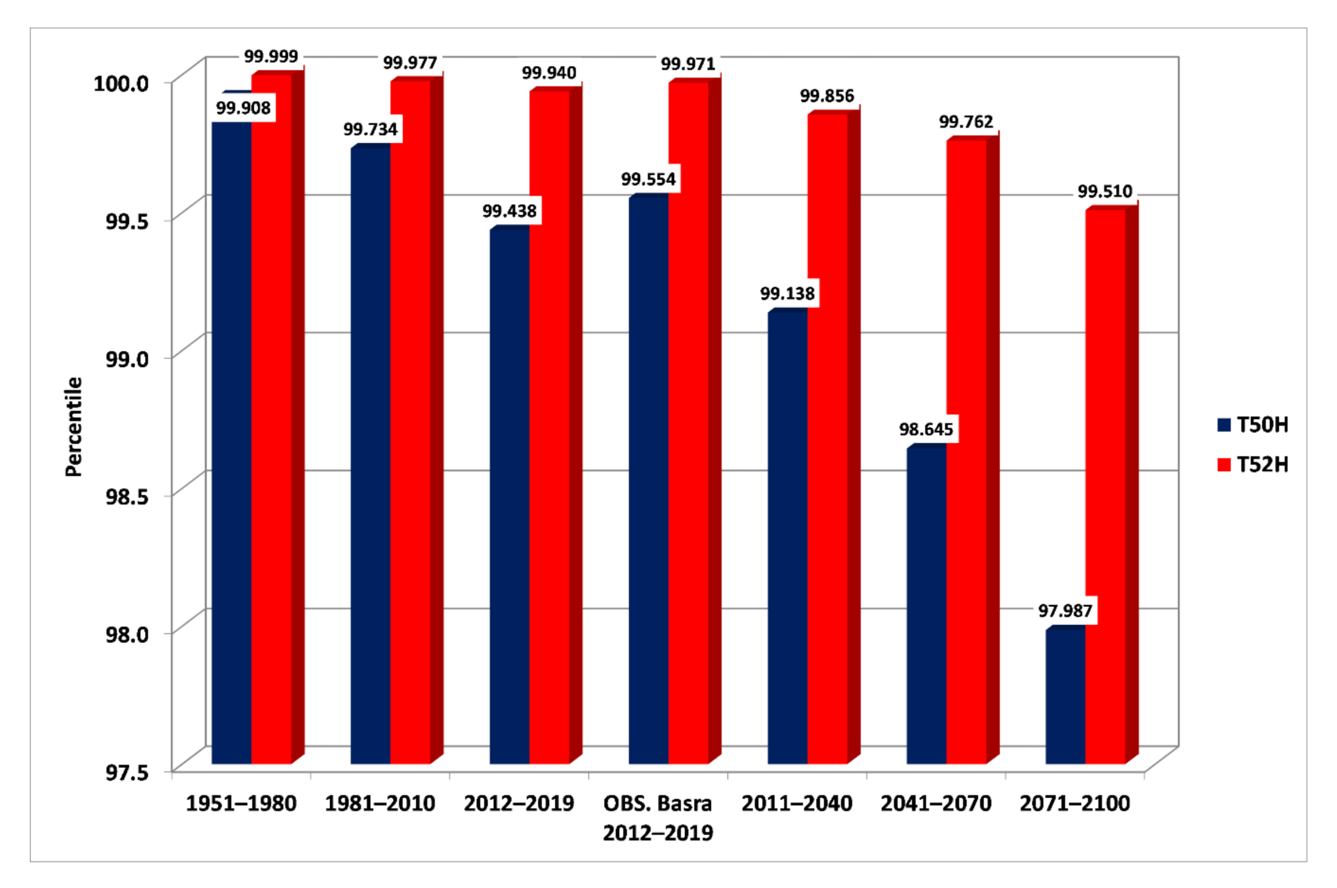
• T50H—the yearly average number of hours with T ≥ 50 °C.
• T52H—the yearly average number of hours with T ≥ 52 °C.
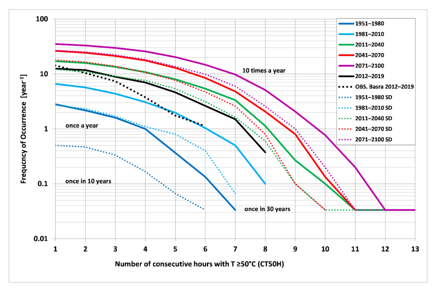
• CT50H—the yearly average number of consecutive hours with T ≥ 50 °C.
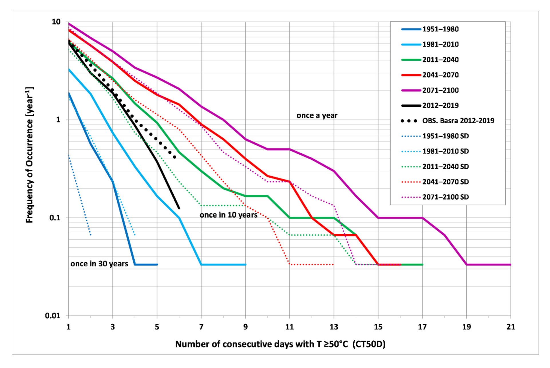
• CT50D—the yearly average number of consecutive days with T ≥ 50 °C.

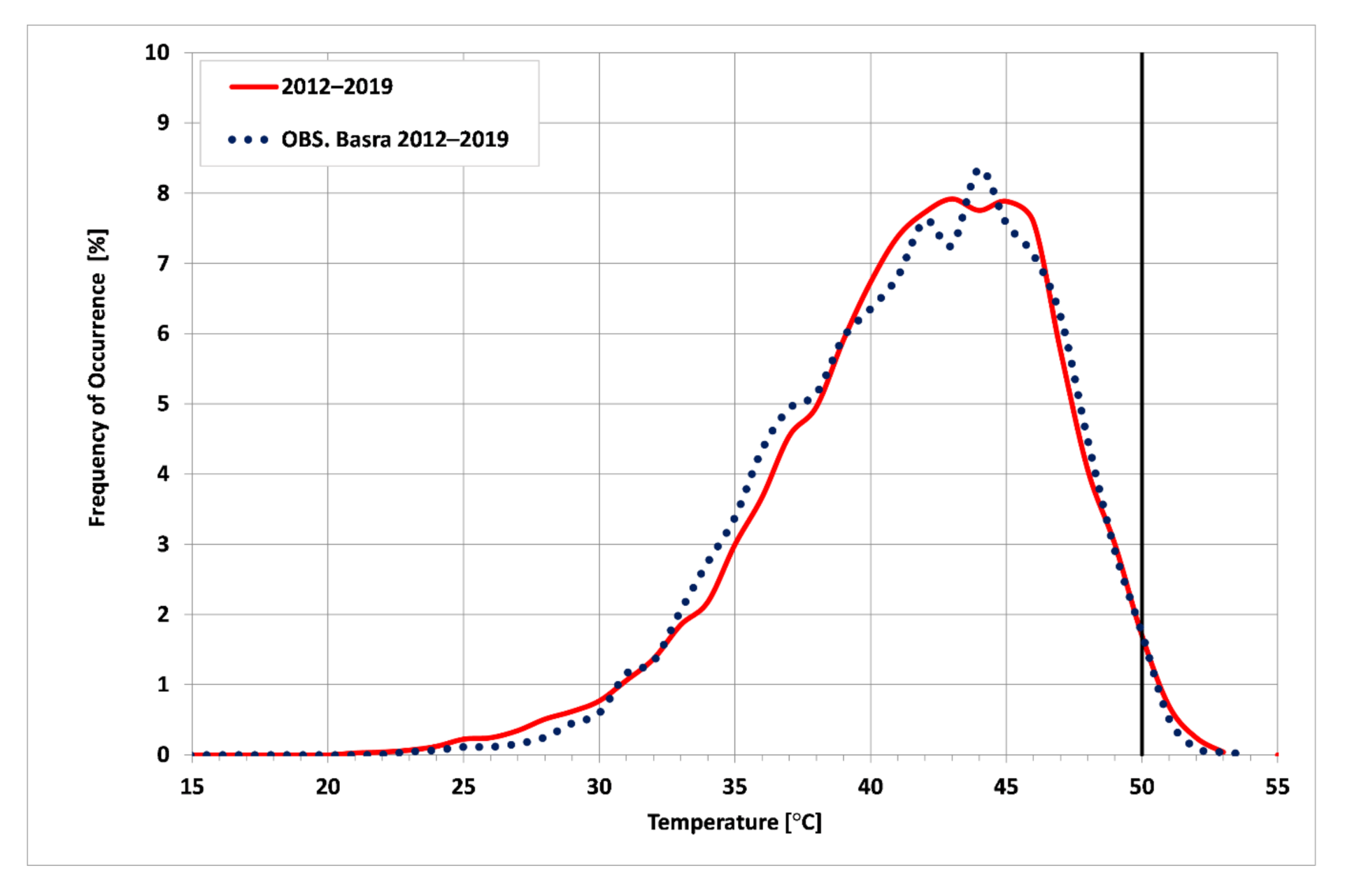
3.2.1. COSMO-CLM and Observed Temperature Distributions

For the eight recent years (2012–2019) with overlapping data between observations and simulated the average observed temperature was 26.74 ± 0.05 °C compared to 27.08 ± 0.05 °C for the simulation. Figure 3 presents the observed and simulated distributions during the daytime (07:00–18:00 UTC) of the summer period (MJJAS). The average observed temperature was 41.38 ± 0.04 °C compared to an average of 41.98 ± 0.04 °C for the simulated data. This slight overestimation of the simulated temperature should be taken into account in the analysis, in the context of all the uncertainties in the projections.

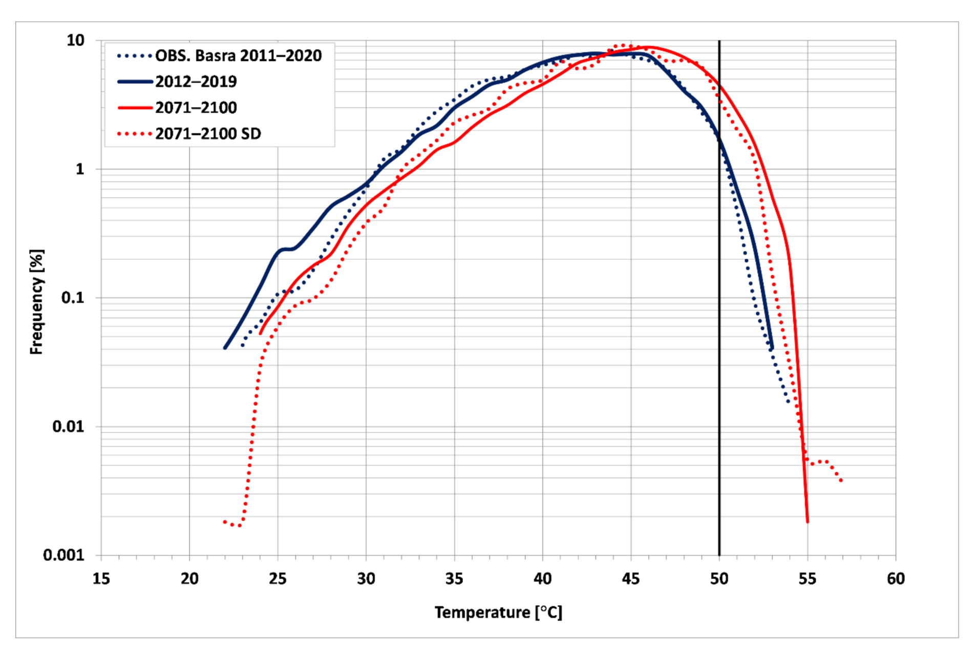
3.2.2. A CDF-t Statistical Downscaling (SD) Attempt

An attempt to analyze the results of CDF-t statistical downscaling for the years 2071–2100 based on the simulated and observed years of 2012–2019 is presented in Figure 4. The frequency of occurrence is presented on a logarithmic scale to emphasize the distribution’s tails. For most of the distributions, the original and the SD values are similar. However, it is evident that the tails of the SD series for 2071–2100 are suspicious. Furthermore, due to the short observed period and its poor quality, the observed curve fluctuates, leading also the SD curve to fluctuant compared to the smoothed direct model output. Although numerous studies have demonstrated that SD methods provide overall value, much less effort has focused on their performance concerning values in the tails of distribution [34]. Therefore, the analysis will concentrate on the direct model output without the CDF-t correction.

3.2.3. Hours Reaching 50 °C and 52 °C or Higher (T50H and T52H)

Table 2. High temperatures statistics between 1951 and 2100.

	Data Source	Max.	Mean	T50H (year−1)	T52H (year−1)	CT50H ≥ 7 h	CT50D ≥ 7 Days
		(period)	(period)			(year−1)	(year−1)
1951–1980	CCLM	52.38	25.77	8.1	0.1	0.03	0
1981–2010	CCLM	53.69	26.5	23.3	2	0.06	0.1
2012–2019	CCLM	53.2	27.08	49.3	5.8	1.88	0
2012–2019	OBS	54	26.74	39.1	2.5	0	0
2011–2040	CCLM	54.79	27.51	75.5	12.6	4.93	1.3
2041–2070	CCLM	55.57	28.39	118.8	20.5	7.83	2.73
2071–2100	CCLM	55.1	28.82	176.5	43	17.97	5.33

summarizes the high temperatures statistics during 150 years including the history runs, the overlapping eight years (2012–2019) of model and observations, together with the projected years assuming the RCP4.5 scenario. The standard WMO recommendation to 30 years periods is the base for the 150 years division. Figure 5 presents the yearly percentiles of T50H and T52H.

For the recent overlapping period, 2012–2019, the simulated average T50H was 49.3 h per year (99.44 percentile) which is 26% higher compared to 39.1 h per year (99.55 percentile) in the observations. For T52H the simulated frequency was double than the observations.

For the 30 years periods the T50H increases 22 times from 8.1 h a year (99.91 percentile) during 1951–1980 to 176.5 h (97.99 Percentile) for the years 2071–2100. In the period 1951–1980 hours with T ≥ 52 °C are a very rare event (99.999 percentile) which occurs once in 10 years. By the end of the century, the projection hours with T ≥ 52 °C will occur 43 times each year, on the average (99.51 percentile).

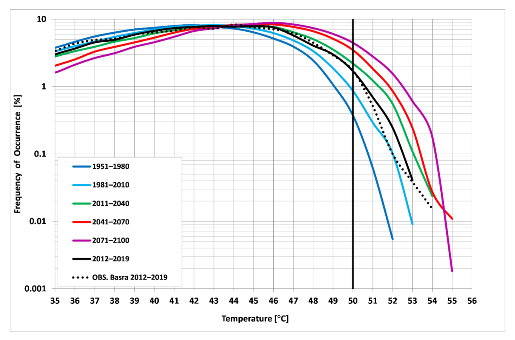
3.2.4. The Right Tail of the Hourly Temperature Distributions

Figure 6 presents the high temperatures distribution for 30 years intervals from 1951 to 2100, together with the overlapping period with observations (2012–2019). The frequency is displayed on a logarithmic scale to emphasize the right tail of the temperature distributions. As in Figure 3 and Figure 4, the right tails of the observed and simulated distributions are quite similar, with a slight overestimation of the simulations for 51 °C and 52 °C. Between 2012 and 2019, the observed record high temperature reached 54 °C on 22 July 2016, while the heights simulated temperature was 53 °C.

It is evident from Figure 6 that from 1951 to 2100 high temperatures above 44 °C are continuously more frequent. The highest temperature recorded in the 30 years intervals of the simulation increased from 52 °C between 1951 and 1980 to 55 °C in the period 2041–2100.

3.2.5. The Number of Consecutive Hours Reaching 50 °C or Higher (CT50H)

Figure 7 displays the DMO projected CT50H together with CT50H after SD, for 30 years intervals from 1951 to 2100. The presentation of the observations during the overlapping period of 2012–2019 enables verification of the simulations. For the recent overlapping period, both the simulated and observed number of consecutive hours reside between the values of 1981–2010 and 2011–2040. Up to three consecutive hours, which occur recently about 10 times a year, the observed and simulated have almost the same values. For higher consecutive hours, the observations contain fewer consecutive hours compared to the simulated.

The CT50H after SD curves seem to be shifted downward by an equivalent of almost 30 years to adjust the positive bias of the model (Table 1, Figure 2 and Figure 4). However, for the low CT50Hs, the SD curve for the years 2011–2040 is below the observed for 2012–2019, which is not logical.

The observed maximal CT50H is six while the DMO simulations reach eight consecutive hours. For the simulated 30-year periods, there is a constant increase in all numbers of CT50H. For the 30 years intervals the longest DMO CT50H increases from seven hours in 1951–1980 to 13 h at 2071–2100 (for one case in 2073, 50 °C was obtained at 19:00 UTC). In the 1951–1980 period, CT50H larger than seven hours was a rare event occurring once in 30 years. At the end of the century, the accumulated days above seven CT50H will occur almost 18 times a year (Table 2).

3.2.6. The Number of Consecutive Days Reaching 50 °C or Higher (CT50D)

Figure 8 is like Figure 7 but for consecutive days reaching 50 °C or higher. As in Figure 7, for the overlapping recent period, 2012–2019, both the simulated DMO and observed number of consecutive days reside between the values of 1981–2010 and 2011–2040. Up to four consecutive days, occurring recently once a year, the observed and simulated DMO have almost the same values. Unlike the long consecutive hours (CT50H), there is an underestimation of the simulated CT50D. For five and six consecutive days, the observations contain eight days compared to only four days in the simulations. For the DMO simulated 30-year periods, there is a constant increase in all CT50D. The longest CT50D in 30 years increased more than four times from a value of five days for the period 1951–1980 to 21 days at the 2071–2100 period. According to the simulations during the 1951–1980 period CT50D larger than seven days never occurred. At the end of the century, the accumulated days above seven CT50D will occur almost 5.3 times a year on average (Table 2).

The CT50D curves after SD are shifted downward more than the CT50H curves after SD. For the years 2011–2040, the SD curves (green dotted line) reside below the observed curve for 2012–2019, leading to the conclusion that the applied SD technique is not accurate enough and DMO may be sufficient.

4. Discussion

There are many uncertainties in future climate projections [35]. The current study uses only one model realization to examine the effect of changing boundary conditions of greenhouse gas concentrations assuming the intermediate CMIP5 RCP4.5 scenario.

Drawing conclusions on the future climate change of an index determined by a temperature threshold implies that the observed and simulated values have the same distribution without any biases. In agreement with Hochman et al. [19] and Luca et al. [36], the comparison of observed and simulated values indicate a slight overestimation of the simulated temperature. Applying the CDF-t caused questionable results for the extreme temperatures and a very strong reduction in consecutive hours and days. For the CT50D the CDF-t results were not reliable or coherent when comparing to the overlapping observations. These findings are in agreement with Lanzante et al. [34] showing that the CDF-t approaches can have sub-optimal performance in the tails, particularly with regard to the maximum value.

Luckily, the research area of southern Iraq is governed by quasi-permanent low-level northwesterly winds (Shamal in Arabic) [37], has a flat terrain, and is free from mesoscale phenomena as sea breeze or mountain flows. Furthermore, the analyzed grid box (Figure 1) contains mainly bare soil where Basra airport is closer to the wetland. Therefore, although there may be a slight overestimation of the simulations compared to the observed values, it can be concluded that even DMO from a model with ~40 km resolution is successful to produce the observed climate distribution. The most recent CMIP6 climate projections for the 21st century indicate a warmer climate compared to CMIP5 despite nominally identical instantaneous radiative forcing [38]. Therefore, the presented slight overestimations of the model may not be far from reality especially if RCP8.5 or CIMP6 are considered. However, as no single CMIP5 nor CMIP6 model stands out as distinctly superior across either temperature or precipitation extremes [39,40], extreme values projections will remain a big challenge also when CMIP6 models will be used for RCM boundary conditions.

Although the current work emphasizes that the COSMO-CLM produces a skillful and plausible representation of climate change, further research is needed. The implementation of extreme value theory such as fitting the generalized extreme value (GEV) distribution [41,42] should be tested. Furthermore, more SD techniques should be tested, including verification that the hourly data of a constantly changing climate fulfills the assumptions that the series are independent and stationary over the 30-year periods.

Salman et al., [20] concluded from the ensemble mean of selected GCMs, that for Iraq the maximum temperatures for the period 2070–2099 will increase in the range of 1.8–4.4 °C relative to the historical period 1971–2000, under the RCP4.5 scenario. The average temperature simulated by COSMO-CLM increased from 1981–2010 to 2071–2100 by 2.3 °C, which is in the lower part of this range. However, the current analysis of extreme temperatures above 50 °C and their consecutive hours and days, reveals that the major climate change feature is not the change in the average temperature.

T50H is projected to increase by a factor of 7.6 from 1981–2010 to 2071–2100 and T52H by a factor of 21.1. Seven or more consecutive hours with T ≥ 50 °C (CT50H) were rare events occurring once in 30 years during 1951–1980. The projection for the end of the century is that such events will occur 18 times a year, on average. Seven or more consecutive days with T ≥ 50 °C (CT50D) were also rare events occurring once in 10 years during 1951–1980. The projection for the end of the century is that such events will occur 5.3 times a year, on average.

5. Conclusions

Our climate variability may be due to natural internal processes within the climate system (internal variability), or to variations in natural or anthropogenic external factors (external variability). Southern Iraq, with flat terrain and without dominant mesoscale phenomena, has low internal variability and may increase the confidence in the projection of external climate conditions due to the addition of greenhouse gas to the atmosphere. The similar distributions of the simulated and observed values demonstrated the possibility to project daily and hourly extremely high temperatures without the need for statistical downscaling.

During the short observational record from Basra airport (2012–2019), the maximum temperature reached 54 °C. The projection for the 60 years 2041 to 2100 includes seven hours with a temperature of 55 °C. New records of high temperatures, although should be expected, are not the major climate change feature. It can be concluded that the main change in the climate of southern Iraq will be the increase in the frequency of occurrence of high temperature (T50H and T52H) and their consecutive occurrence (CT50H and CT50D). These findings should be easier to internalize for most people who have difficulty to feel an average increase of two or three degrees as most climate change papers state.

These findings suggest that there is a need for global mitigation measures to reduce and curb greenhouse gas emissions, and local adaptation measures to reduce the vulnerability of heat waves. With the lack of local adaptation measures, the impact of increasing extreme temperature frequency may spark political unrest.

References

1. Zerboni, A.; Biagetti, S.; Lancelotti, C.; Madella, M. The end of the Holocene Humid Period in the central Sahara and Thar deserts: Societal collapses or new opportunities? Past Glob. Chang. Mag. 2016, 24, 60–61. [Google Scholar] [CrossRef] [Green Version]
2. Staubwasser, M.; Weiss, H. Holocene climate and cultural evolution in late prehistoric–early historic West Asia. Quat. Res. 2006, 66, 372–387. [Google Scholar] [CrossRef] [Green Version]
3. Fuks, D.; Ackermann, O.; Ayalon, A.; Bar-Matthews, M.; Bar-Oz, G.; Levi, Y.; Maeir, A.M.; Weiss, E.; Zilberman, T.; Safrai, Z. Dust clouds, climate change and coins: Consiliences of palaeoclimate and economy in the Late Antique southern Levant. Levant 2017, 49, 205–223. [Google Scholar] [CrossRef]
4. Schär, C. Climate extremes: The worst heat waves to come. Nat. Clim. Chang. 2016, 6, 128–129. [Google Scholar] [CrossRef]
5. Epstein, Y.; Moran, D.S. Extremes of temperature and hydration. In Travel Medicine; Elsevier: Amsterdam, The Netherlands, 2019; pp. 407–415. [Google Scholar] [CrossRef]
6. Tasian, G.E.; Pulido, J.E.; Gasparrini, A.; Saigal, C.S.; Horton, B.P.; Landis, J.R.; Madison, R.; Keren, R. Urologic Diseases in America Project, Daily mean temperature and clinical kidney stone presentation in five US metropolitan areas: A time-series analysis. Environ. Health Perspect. 2014, 122, 1081–1087. [Google Scholar] [CrossRef] [PubMed] [Green Version]
7. Golomb, D.; Goldberg, H.; Nevo, A.; Lavi, A.; Zelichenko, G.; Cohen, M.; Kafka, I.; Chertin, B.; Lezarovic, A.; Kleinman, N.; et al. MP03-18 DO weather parameters affect the incidence of renal colic in a predominantly warm country? A multicenter ecological study. J. Urol. 2020, 203, e29–e30. [Google Scholar] [CrossRef]
8. Basagaña, X.; Michael, Y.; Lensky, I.; Rubin, L.; Haklai, Z.; Grotto, I.; Vadislavsky, E.; Levi, Y.; Amitai, E.; Agay-Shay, K. Identifying windows of susceptibility during pregnancy: Associations between low and high ambient temperature and birth weight for 609,886 singleton term births born in Israel during 2010–2014. Environ. Health Perspect. (Submitted 2020).
9. Zhao, C.; Liu, B.; Piao, S.; Wang, X.; Lobell, D.B.; Huang, Y.; Huang, M.; Yao, Y.; Bassu, S.; Ciais, P.; et al. Temperature increase reduces global yields of major crops in four independent estimates. Proc. Natl. Acad. Sci. USA 2017, 114, 9326–9331. [Google Scholar] [CrossRef] [Green Version]
10. Lesk, C.; Rowhani, P.; Ramankutty, N. Influence of extreme weather disasters on global crop production. Nature 2016, 529, 84–87. [Google Scholar] [CrossRef]
11. Dahlquist, R.M.; Prather, T.S.; Stapleton, J.J. Time and temperature requirements for weed seed thermal death. Weed Sci. 2007, 55, 619–625. [Google Scholar] [CrossRef]
12. Hanna, E.G.; Tait, P.W. Limitations to thermoregulation and acclimatization challenge human adaptation to global warming. Int. J. Environ. Res. Public Health 2015, 12, 8034–8074. [Google Scholar] [CrossRef] [PubMed]
13. Sherwood, S.C.; Huber, M. An adaptability limit to climate change due to heat stress. Proc. Natl. Acad. Sci. USA 2010, 107, 9552–9555. [Google Scholar] [CrossRef] [Green Version]
14. Pal, J.S.; Eltahir, E.A. Future temperature in southwest Asia projected to exceed a threshold for human adaptability. Nat. Clim. Chang. 2016, 6, 197. [Google Scholar] [CrossRef]
15. Azooz, A.A.; Talal, S.K. Evidence of climate change in Iraq. J. Environ. Prot. Sustain. Dev. 2015, 1, 66–73. [Google Scholar]
16. Salman, S.A.; Shahid, S.; Ismail, T.; Chung, E.S.; Al-Abadi, A.M. Long-term trends in daily temperature extremes in Iraq. Atmos. Res. 2017, 198, 97–107. [Google Scholar] [CrossRef]
17. Bucchignani, E.; Cattaneo, L.; Panitz, H.J.; Mercogliano, P. Sensitivity analysis with the regional climate model COSMO-CLM over the CORDEX-MENA domain. Meteorol. Atmos. Phys. 2016, 128, 73–95. [Google Scholar] [CrossRef]
18. Bucchignani, E.; Mercogliano, P.; Panitz, H.J.; Montesarchio, M. Climate change projections for the Middle East–North Africa domain with COSMO-CLM at different spatial resolutions. Adv. Clim. Chang. Res. 2018, 9, 66–80. [Google Scholar] [CrossRef]
19. Hochman, A.; Bucchignani, E.; Gershtein, G.; Krichak, S.O.; Alpert, P.; Levi, Y.; Yosef, Y.; Zollo, A.L. Evaluation of regional COSMO-CLM climate simulations over the Eastern Mediterranean for the period 1979–2011. Int. J. Climatol. 2018, 38, 1161–1176. [Google Scholar] [CrossRef]
20. Salman, S.A.; Shahid, S.; Ismail, T.; Ahmed, K.; Wang, X.J. Selection of climate models for projection of spatiotemporal changes in temperature of Iraq with uncertainties. Atmos. Res. 2018, 213, 509–522. [Google Scholar] [CrossRef]
21. Meehl, G.A.; Tebaldi, C. More intense, more frequent, and longer lasting heat waves in the 21st century. Science 2004, 305, 994–997. [Google Scholar] [CrossRef] [Green Version]
22. Boisserie, M.; Arbogast, P.; Descamps, L.; Pannekoucke, O.; Raynaud, L. Estimating and diagnosing model error variances in the Météo-France global NWP model. Q. J. R. Meteorol. Soc. 2014, 140, 846–854. [Google Scholar] [CrossRef]
23. Pierce, D.W.; Cayan, D.R.; Maurer, E.P.; Abatzoglou, J.T.; Hegewisch, K.C. Improved bias correction techniques for hydrological simulations of climate change. J. Hydrometeorol. 2015, 16, 2421–2442. [Google Scholar] [CrossRef]
24. Yosef, Y.; Aguilar, E.; Alpert, P. Is it possible to fit extreme climate change indices together seamlessly in the era of accelerated warming? Int. J. Climatol. 2020. [CrossRef]
25. Thrasher, B.; Maurer, E.P.; McKellar, C.; Duffy, P.B. Bias correcting climate model simulated daily temperature extremes with quantile mapping. Hydrol. Earth Syst. Sci. 2012, 16, 3309–3314. [Google Scholar] [CrossRef] [Green Version]
26. Maraun, D. Bias correction, quantile mapping, and downscaling: Revisiting the inflation issue. J. Clim. 2013, 26, 2137–2143. [Google Scholar] [CrossRef] [Green Version]
27. Michelangeli, P.A.; Vrac, M.; Loukos, H. Probabilistic downscaling approaches: Application to wind cumulative distribution functions. Geophys. Res. Lett. 2009, 36, 11. [Google Scholar] [CrossRef]
28. Rockel, B.; Will, A.; Hense, A. The regional climate model COSMO-CLM (CCLM). Meteorol. Z. 2008, 17, 347–348. [Google Scholar] [CrossRef]
29. Giorgi, F.; Jones, C.; Asrar, G.R. Addressing climate information needs at the regional level: The CORDEX framework. World Meteorol. Organ. Bull. 2009, 58, 175. [Google Scholar]
30. Dee, D.P.; Uppala, S.M.; Simmons, A.J.; Berrisford, P.; Poli, P.; Kobayashi, S.; Andrae, U.; Balmaseda, M.A.; Balsamo, G.; Bauer, P.; et al. The ERA-Interim reanalysis: Configuration and performance of the data assimilation system. Q. J. R. Meteorol. Soc. 2011, 137, 553–597. [Google Scholar] [CrossRef]
31. Stevens, B.; Giorgetta, M.; Esch, M.; Mauritsen, T.; Crueger, T.; Rast, S.; Salzmann, M.; Schmidt, H.; Bader, J.; Block, K.; et al. Atmospheric component of the MPI-M Earth system model: ECHAM6. J. Adv. Modeling Earth Syst. 2013, 5, 146–172. [Google Scholar] [CrossRef]
32. Ishizaki, Y.; Shiogama, H.; Emori, S.; Yokohata, T.; Nozawa, T.; Ogura, T.; Abe, M.; Yoshimori, M.; Takahashi, K. Temperature scaling pattern dependence on representative concentration pathway emission scenarios. Clim. Chang. 2012, 112, 535–546. [Google Scholar] [CrossRef] [Green Version]
33. Lavaysse, C.; Vrac, M.; Drobinski, P.; Lengaigne, M.; Vischel, T. Statistical downscaling of the French Mediterranean climate: Assessment for present and projection in an anthropogenic scenario. Nat. Hazards Earth Syst. Sci. 2012, 12, 651–670. [Google Scholar] [CrossRef] [Green Version]
34. Lanzante, J.R.; Nath, M.J.; Whitlock, C.E.; Dixon, K.W.; Adams-Smith, D. Evaluation and improvement of tail behaviour in the cumulative distribution function transform downscaling method. Int. J. Climatol. 2019, 39, 2449–2460. [Google Scholar] [CrossRef] [Green Version]
35. Tebaldi, C.; Knutti, R. The use of the multi-model ensemble in probabilistic climate projections. Philos. Trans. R. Soc. A Math. Phys. Eng. Sci. 2007, 365, 2053–2075. [Google Scholar] [CrossRef]
36. Di Luca, A.; Pitman, A.J.; de Elía, R. Decomposing Temperature Extremes Errors in CMIP5 and CMIP6 Models. Geophys. Res. Lett. 2020, 47, e2020GL088031. [Google Scholar] [CrossRef]
37. Francis, D.B.K.; Flamant, C.; Chaboureau, J.P.; Banks, J.; Cuesta, J.; Brindley, H.; Oolman, L. Dust emission and transport over Iraq associated with the summer Shamal winds. Aeolian Res. 2017, 24, 15–31. [Google Scholar] [CrossRef]
38. Wyser, K.; Kjellström, E.; Koenigk, T.; Martins, H.; Döscher, R. Warmer climate projections in EC-Earth3-Veg: The role of changes in the greenhouse gas concentrations from CMIP5 to CMIP6. Environ. Res. Lett. 2020, 15, 054020. [Google Scholar] [CrossRef]
39. Wehner, M.; Gleckler, P.; Lee, J. Characterization of long period return values of extreme daily temperature and precipitation in the CMIP6 models: Part 1, model evaluation. Weather Clim. Extrem. 2020, 30, 100283. [Google Scholar] [CrossRef]
40. Wehner, M.F. Characterization of long period return values of extreme daily temperature and precipitation in the CMIP6 models: Part 2, projections of future change. Weather Clim. Extrem. 2020, 30, 100284. [Google Scholar] [CrossRef]
41. Kysel, J. Comparison of extremes in GCM-simulated, downscaled and observed central-European temperature series. Clim. Res. 2002, 20, 211–222. [Google Scholar] [CrossRef]
42. Katz, R.W. Statistics of extremes in climate change. Clim. Chang. 2010, 100, 71–76. [Google Scholar] [CrossRef]
Figure 1. A Google Earth map of the study area including the COSMO-CLM (consortium for small-scale modelling—climate limited area modelling) grid point (red) which was compared to the observation from Basra airport.
Atmosphere 11 01155 g001
Figure 2. Maximum daily temperature (Tmax) simulated by COMO-CLM driven by ERA-Interim reanalysis as a function of observed maximum temperature in Basra airport. The red lines for the Tmax = 50 °C threshold divide the domain as by the contingency table (Table 1).
Atmosphere 11 01155 g002
Figure 3. Frequency of occurrence of hourly temperatures in Southern Iraq simulated by COSMO-CLM and observed from Basra airport from May to September (MJJAS) between 07:00 and 18:00 UTC for the years 2012–2019.
Atmosphere 11 01155 g003
Figure 4. Frequency of occurrence of hourly temperatures in southern Iraq simulated by COSMO-CLM for 2071–2100 with and without statistical downscaling (SD), and for the year’s 2012–2019 as in Figure 3 but on a logarithmic scale. The data is for MJJAS between 07:00 and 18:00 UTC.
Atmosphere 11 01155 g004
Figure 5. The yearly percentile values of hours with T ≥ 50 °C (T50H) and T ≥ 52 °C (T52H) for different projection periods and the observation in Basra airport during 2012–2019.
Atmosphere 11 01155 g005
Figure 6. The simulated and observed (black dots) frequency of occurrence of hourly high temperatures in southern Iraq near Basra during MJJAS between 07:00 and 18:00 UTC.
Atmosphere 11 01155 g006
Figure 7. The average yearly frequency of consecutive hours with the temperature reaching 50 °C or higher (CT50H) for 30 years intervals obtained by the COSMO-CLM and for the eight overlapping years (2012–2019) with the observations from Basra airport. The lines represent the direct model output and the dotted lines are after SD. The black dots represent the observations from Basra airport. The last point in each line indicates the maximum consecutive hours in each period.
Atmosphere 11 01155 g007
Figure 8. As in Figure 7 for consecutive days with 50 °C and above (CT50D).
Atmosphere 11 01155 g008