Abstract
A hot blob for near-surface water was identified eastward of New Zealand in the South Pacific in December 2019, which was the second strongest event on record in this region. Its sea surface temperature anomalies reached up to 5 °C, and the anomalous warming penetrated around 40 m deep vertically. From the atmospheric perspective, the anomalous high-pressure system from the surface up to 300 hPa lasted for about 50 days, accompanied by the blocking pattern at 500 hPa and a deep warming air column extending downward to the surface. A mixed-layer heat budget analysis revealed that the surface heat flux term was the primary factor contributing to the development of this hot blob, with more shortwave radiation due to the persistent high-pressure system and lack of clouds as well as higher temperature of the troposphere aloft denoted by sensible heat. The oceanic contribution including the horizontal advection and vertical entrainment was changeable and accounted for less than 50%. Moreover, we used the strongest hot blob event which peaked in December 2001 as another example to evaluate the robustness of results derived from the 2019 case. The results show similar circulation features and driving factors, which indicate the robustness of the above characteristics.
1. Introduction
Regional summer heatwaves have occurred more frequently over the globe since 2000 [1,2,3,4], which has attracted wide attention among researchers. Moreover, marine heatwave days have increased 54% globally since the early 20th century, according to the definition of Hobday et al. [5], in particular with an increase of 3–9 days per decade in the New Zealand region [6]. Recently in December 2019, a hot blob (also termed “marine heatwave”) appeared and spanned at least a million square kilometers—an area nearly four times larger than New Zealand—in the South Pacific (Figure 1a). This remarkable spike in sea surface temperature (SST) reached up to 5 °C above average across a massive patch and was located to the east of New Zealand, near the sparsely populated Chatham Islands archipelago. In addition, it was the biggest patch of anomalous warming over global oceans at that time. As the news reported, this New Zealand “marine heatwave” brought tropical fish from 3000 km away [7]. This surge in ocean heat over a short period could have been difficult for local marine life if it had penetrated far beyond the surface. This record-breaking hot blob followed a marine heatwave two summers ago that propelled the hottest summer of New Zealand on record, more than 3 °C above average SST, and led to tropical fish from Australia being found along the country’s coast [8]. Furthermore, Salinger et al. [9] analyzed three unparalleled coupled ocean–atmosphere heatwaves around the New Zealand region during the austral summers of 1934/1935, 2017/2018 and 2018/2019.
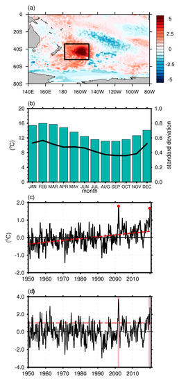
Figure 1.
(a) The sea surface temperature anomaly (SSTA) (shading, in °C) in South Pacific on 25 December 2019. Black box indicates the blob area (34° S–52° S, 150° W–178° W). (b) The climatological monthly SST (green bar, left axis, in °C) averaged over blob area. The black line depicts its monthly SD (right axis). (c) The SSTA time series of blob area from 1950 to 2019. Red-dashed line indicates its linear trend using linear regression. The red dots represent the values in December 2001 and 2019, respectively. (d) The normalized SSTA time series of the blob area from 1950 to 2019. The pink shading indicates the duration of two extreme cases when the time series was larger than 1.0 SD. The red dashed line denotes the threshold of 1.0 SD.
Heatwaves are natural hazards that have substantial impacts on human health, the economy and the environment in both the atmosphere and ocean [10]. For example, the 2011 marine heatwave in Western Australia exerted great effects on marine biodiversity [11,12] while the ones near New Zealand also caused the rapid loss of snow and glacier ice and largely affected the agriculture [8,9]. In the Northern Hemisphere, the record-breaking warm and persistent water mass in the Northeastern Pacific during 2013–2015, termed the “Pacific warm blob” [13] and “marine heatwave” [14,15], also had catastrophic influences on the climate, coastal ecosystems and fisheries [16,17], which led to the anomalously warm winter in Alaska [18] but colder winter in wide regions of North America [19], the migration of marine species [20,21], a large amount of dead species [20,22], and the shutdown of local fisheries [23], as well as possibly the severe drought in California [24]. However, the underlying physical mechanisms of marine heatwaves are less well understood. Several reasons are documented to be the potential drivers: El Niño-Southern Oscillation (ENSO) [11,14,25], mesoscale eddies [26], oceanic heat advection/transport [27,28], high atmospheric temperatures and low local winds [13,29,30,31]. However, research into marine heatwaves is still in its infancy, with little consensus about the driving mechanisms [10].
In short, many issues remain unresolved about the marine heatwaves in the South Pacific. Given that there have been more and more local events in recent years [11] and their associated disasters, considerable efforts are required to illuminate their driving mechanisms and generate future projections of marine heatwaves [9]. In this study, we took the recent hot blob eastward of New Zealand in December 2019 as an example and analyzed its synoptic characteristics and heat budgets, aiming to quantify the contributions from atmosphere and ocean. Moreover, we used another hot blob event in December 2001, the strongest event east of New Zealand on record, as another example to have a comparison and further prove the robustness of circulation anomalies and the leading driving factor derived from the recent December 2019 case.
2. Data and Methods
We employed both daily and monthly data to illustrate the hot blob events in this study. The atmospheric data were obtained from the National Centers for Environmental Prediction-National Center for Atmospheric Research (NCEP-NCAR) Reanalysis 1 [32,33,34]. They had a horizontal resolution of 2.5° × 2.5° in latitude and longitude, with 17 standard pressure levels vertically. The climatology is the mean state computed by averaging the 30-year data from 1990 to 2019. We used the departure from the climatology as anomalies according to Shi and Qian [35]. The variables including the air temperature, sea level pressure (SLP), geopotential height, surface winds, and heat fluxes in this study.
For the SST data, we utilized the monthly Extended Reconstructed Sea Surface Temperature (ERSST) V5 data in a 2° × 2° horizontal resolution from the National Oceanic and Atmospheric Administration (NOAA) [36,37]. The monthly SST climatology was constructed by averaging the SST from 1950 to 2019. The daily SST dataset was retrieved from the Optimum Interpolation (OISST) with a 0.25° × 0.25° horizontal resolution [38]. The subsurface temperature and current velocity data were obtained from the NCEP Global Ocean Data Assimilation System (GODAS) [39,40]. We also used Argo subsurface temperature for comparison [41]. We further calculated the anomaly of specific variable as the difference between the total value and the corresponding climatology.
The focused blob area covered (34° S–52° S, 150° W–178° W) in the South Pacific. For the definition of marine heatwaves, Hobday et al. [5] proposed a comprehensive one considering an anomalously warm event to be a marine heatwave if it lasts for five or more days, with temperatures warmer than the 90th percentile based on a 30-year historical baseline period. However, we did not apply this definition because we do not focus on the detailed daily evolution of the hot blob cases in December 2001 and 2019. Instead, we give a relatively wide picture of the blobs especially in the mixed-layer heat budget analysis, which is illustrated using the monthly data.
To quantify the relative contribution of at mospheric and oceanic processes in above hot blob events, we employed the mixed-layer heat budget analysis in November and December of 2019 according to Cronin et al. [42] and Schmeisser et al. [43]. As shown in Equation (1) below,
where T is the SST anomaly (SSTA) over the blob area derived from ERSST V5 and the first term indicates the tendency of SST. Q0 is the net heat flux at the ocean–atmosphere interface, which is the sum of the net shortwave radiation flux (SW), net longwave radiation flux (LW), net latent heat flux (LH), and sensible heat net flux (SH). The heat fluxes were regridded from NCEP-NCAR Reanalysis 1 to a 1° × 1° horizontal resolution using linear interpolation. All the heat flux terms were converted into positive downwards to indicate the favorable condition for blob warming. The describes the heat capacity of water () and h is the long-term mean mixed layer depth via the potential temperature in a 1° × 1° horizontal resolution from the NODC (Levitus) World Ocean Atlas 1994 [44,45]. The second and third terms on the right–hand side of equation (1) represent the oceanic horizontal advection in the mixed layer and vertical entrainment at the bottom of the mixed layer, respectively. It should be noted that we did not explicitly calculate the vertical entrainment in this study in part due to the lack of ocean subsurface data and we obtained this term as the residual by removing the heat flux and advection terms from the SST tendency term. More details can be found in Cronin et al. [42] and Schmeisser et al. [43]. In addition, the least-squares linear regression method is utilized to estimate the linear trends of regional blob variation.
3. Results
3.1. Features of the Hot Blob Eastward of New Zealand in December 2019
Firstly, we inspected the annual cycle of the SST (Figure 1b) in the blob area of the South Pacific (black box in Figure 1a). In December, the climatological SST is around 14 °C, followed by the hottest months of January, February, and March. Due to the anomalous warming in 2019, the local SST could reached 20 °C in December. Moreover, the SST standard deviation (SD) in this region is large in December, indicating a relatively larger natural variability at this time.
Furthermore, the historical context in this blob area was given by the monthly SSTA from January 1950 to December 2019 (Figure 1c). Within this area, an extreme hot blob event was presented in December 2019 with SSTA about 2.8 times the SD warmer than the climatological SST (also see Figure 1d). Clearly, it is common to see patches of warmer water off New Zealand, but this magnitude is the second largest on record. The event that occurring in December 2001 was the strongest case during our study period (Figure 1c). These two events were prominent in magnitude compared to the SSTA at other times. It should be noted that the above two events both occurred in December, implying the potential phase-locking feature of hot blobs in this area during austral summer. On the other hand, there is a prominent increasing trend of SSTs in this blob region (Figure 1c), partly contributing to the extreme magnitude of these two blob events. In addition, this significant warming trend is very consistent with the global warming tendency. To depict the duration of the two extreme hot blobs, we calculated the normalized monthly SSTA averaged over the blob area (Figure 1d). Both of them are long-lived events in a monthly-based context if we take 1.0 as the threshold. The duration of the 2001 event is 11 months, while it is 10 months for the recent 2019 event (pink shading in Figure 1d).
Figure 2 further illustrates the depth of the hot blobs using both monthly GODAS and Argo data. The positive temperature anomalies greater than 0.5 °C could penetrate into approximately 40 m in December 2019 (Figure 2a,b,d,e). Similarly, the depth of warmer-than-normal subsurface water outlined by the 0.5 °C contour was also shallower than 50 m in December 2001 (Figure 2c,f). By comparison, the vertical penetration of the hot blobs east of New Zealand appeared much shallower than that of the record-breaking warm blob in Northeastern Pacific during 2013–2015 (around 200–250 m according to Hu et al. [46]). Therefore, the similarity and difference of the hot blobs (or marine heatwaves) in two hemispheres should be further compared and illustrated.
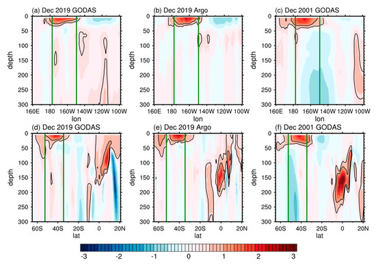
Figure 2.
The depth-longitude vertical section of subsurface temperature anomalies (shading and contour, 0.5 °C and 1.0 °C highlighted) averaged over 34° S–52° S in (a) December 2019 using GODAS data, (b) December 2019 using Argo data, and (c) December 2001 using GODAS data, respectively. (d–f) Same as (a–c), but for depth-latitude section averaged over 150° W–178° W. The green vertical lines outline the blob area.
Climatologically, westerlies prevail over the entire blob region, which is located to the southwest of the subtropical high (Supplementary Materials Figure S1). The subtropical high gradually weakens from November to December, associated with the weakening of westerlies in the blob area. Figure 3 illustrates the evolution of SLP and surface wind anomalies as well as total geopotential heights at 500 hPa every 10 days from 1 November to 31 December of 2019. The surface high system persisted from mid-November to late December (Figure 3). The easterly anomalies weakened the climatological westerlies (Figure 3c–e) and thus reduced the heat loss of the ocean via similar processes involved in a wind–evaporation–SST (WES) mechanism [47], favorable for the warming of local SST. From the oceanic perspective, the easterly anomalies transported the warmer water from tropics via Ekman transport (Figure 3c–e), which also contributed to the positive SSTA of the blob region. Furthermore, there was less rainfall and dry weather under the continuous anticyclonic condition, causing more shortwave radiation to come to and heat the ocean surface. We notice that although the anomalous surface high was long-lasting, the wind anomalies within the blob area were a bit more variable (Figure 3). In terms of the geopotential heights at 500 hPa, a prominent ridge was stable with a blocking pattern during the middle December of 2019 (Figure 3e). The importance of the blocking characteristic during a marine heatwave has also been documented in Salinger et al. [8,9].
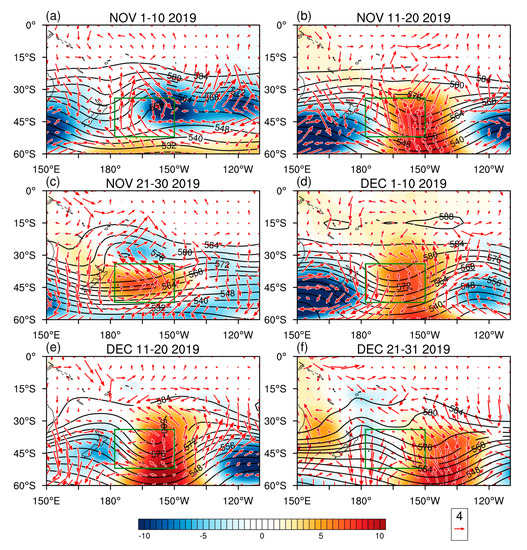
Figure 3.
Sea level pressure (SLP) anomalies (shading, in hPa), surface wind anomalies (vector, in m/s), and total geopotential heights at 500 hPa (black contour, in dagpm) averaged over (a) 1–10 November, (b) 11–20 November, (c) 21–30 November, (d) 1–10 December, (e) 11–20 December and (f) 21–31 December of 2019. The green boxes denote the blob area.
To further reveal the atmospheric characteristics during November and December of 2019, we ploted the evolution of the temperature and geopotential height anomalies in the vertical direction averaged over the blob region (Figure 4a). Similar illustrations are widely used in investigating extreme warm events in the atmosphere [35,48]. The anomalous warming was strongest at the middle-lower troposphere, with a deep-warm air column extending upward to 300 hPa and downward to the surface. This persistent warming in the troposphere benefited the outstanding SST warming in the blob area in December 2019 through air-sea interaction (Figure 4a). The surface high-pressure system in Figure 3 corresponded to the long-lasting anomalous high circulation centered at around 300 hPa (Figure 4a). The anomalous high circulation and warming lasted for around 50 days and formed a prominent intraseasonal signal from the atmospheric perspective. We conclude that the atmospheric height and temperature configuration could stimulate the positive SSTA in the blob area.
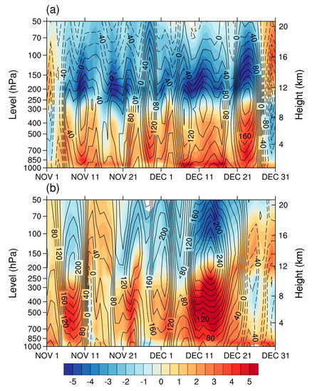
Figure 4.
The temporal evolution of air temperature anomalies (shading, in °C) and geopotential height anomalies (contour, in gpm) averaged over the blob area from 1 November to 31 December of (a) 2019 and (b) 2001, respectively.
3.2. Mixed-Layer Heat Budget of the Hot Blob Event in November and December 2019
In November, the SST of the blob area was warmed primarily due to the positive heat flux from the atmosphere, with most of the contributions from the SW and SH (Figure 5). The contribution of horizontal advection in the mixed layer was positive with a generally equivalent value compared with the temperature tendency. However, the vertical entrainment and diffusion processes played a negative role in warming the blob region at this stage, which largely offset the positive contribution from the heat fluxes at the ocean–atmosphere interface. Then during December, there was a much larger warming tendency for the blob SST (Figure 5), associated with the quick development and occurrence of the hot blob in Figure 1a. Quantitatively, the atmosphere and ocean played a generally equal role in this blob event (Figure 5). More SW penetrated the ocean surface and therefore heated the blob area due to the deep high-pressure system (Figure 4a) and lack of clouds. The positive SH anomaly contributed nearly 50% of the total heat flux term, which resulted from the direct heating of warmer tropospheric column aloft (Figure 4a). We notice that the influence of oceanic processes reversed from negative in November to positive in December, possibly implying the seasonal variability of the upper ocean or a change in its internal thermodynamic properties, which needs further investigation.
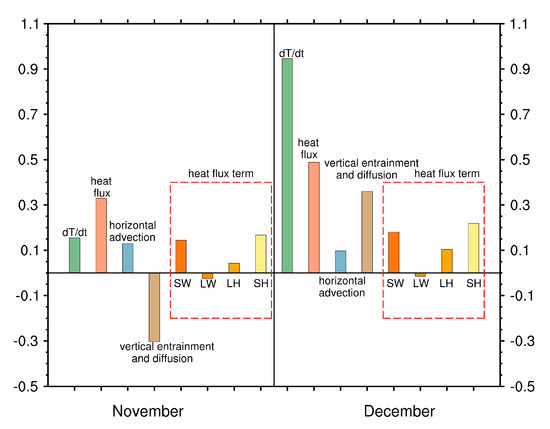
Figure 5.
The heat budget (in °C/mon) of blob area in November and December of 2019. The “dT/dt” term is the tendency of SST (green bar), while the “heat flux” term (pink bar) is from atmosphere, “horizontal advection” term (blue bar), and “vertical entrainment and diffusion” term (brown bar) are calculated in the ocean mixed layer. In addition, the specific SW, LW, LH, SH terms are calculated and represented within the red-dashed box. All the heat flux terms are defined as positive downwards.
3.3. Comparison of the Historical Strongest Hot Blob in December 2001
To evaluate the robustness of the above results, we further analyzed the strongest hot blob event that occurred in December 2001 (Figure 1c). In terms of the SLP and surface wind anomalies, the favorable anti-clockwise circulation anomalies were persistent from early November to middle-late December of 2001 (Figure 6). The easterly anomalies to the north of the above surface high system counteracted the climatological westerlies, reduced the evaporation and latent heat loss of the ocean, and heated the ocean surface in the blob area, which was similar to the WES mechanism. In the Southern Hemisphere, the easterly wind anomalies could advect the warmer water from lower latitudes to the blob area via Ekman transport, which also contributed to the positive SSTA of the blob region. Importantly, the blocking feature at 500 hPa was more evident (Figure 6e) compared to that in 2019 (Figure 3e), in accordance with their intensity difference. From the vertical section averaged over the blob area, we observed a significant warming in the troposphere aloft (Figure 4b), which warmed the oceanic surface through the sensible heat fluxes (Figure 7). This heating effect was especially intensive during the middle of December, with a warm core greater than 5 °C centered at around 400–500 hPa (Figure 4b). Correspondingly, the magnitude of the positive height anomalies was much greater compared to that in December 2019 (Figure 4a). The above anomalous height and temperature configuration satisfied the hydrostatic balance according to previous studies [35,48].
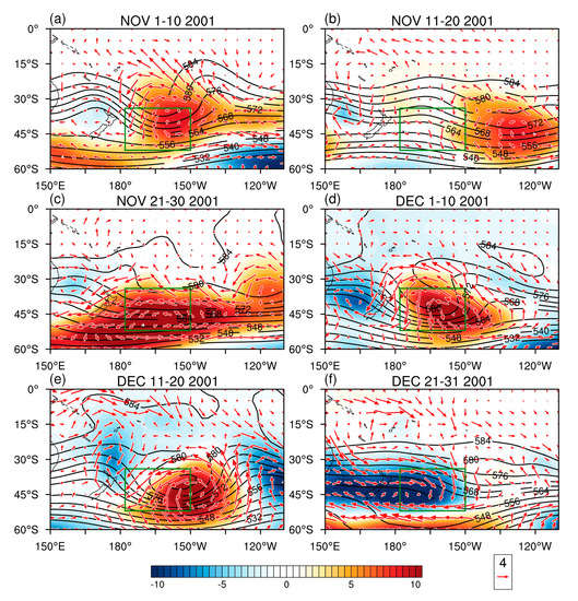
Figure 6.
Same as Figure 3, but for 2001 case.
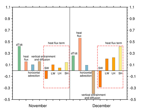
Figure 7.
Same as Figure 5, but for November and December of 2001.
Then, we conducted similar mixed-layer heat budget analysis for this hot blob event (Figure 7). In November 2001, the surface heat fluxes and oceanic vertical processes were mostly responsible for the early warming of this hot blob. Then in December, the heat fluxes became much larger, with a dominant positive SH anomaly indicating the heating from the atmosphere (Figure 7). Moreover, the LH anomalies also became more prominent and favorable for the intensification of this hot blob, which was related to the easterly anomalies and the resultant lower evaporation and LH loss. Similar to the December 2019 case (Figure 5), the vertical entrainment and diffusion term also changed sign during these two months, which implied a possible complexity of oceanic processes during austral summer. The horizontal advection played a positive role in both November and December but with a limited magnitude (Figure 7).
4. Discussion
A hot blob with the SSTA reaching up to 5 °C on specific days occurred eastward of New Zealand in the South Pacific in December 2019 and was reported to be the biggest warming patch over global oceans at that time. Moreover, this blob was shown to be the second largest event on record in this region. The sudden warming of this hot blob was primarily contributed by the atmosphere, with positive heating due to the higher temperature of the troposphere aloft denoted by sensible heat as well as more shortwave radiation due to the persistent high-pressure system and, potentially, the lack of clouds. From the oceanic perspective, the vertical entrainment and diffusion processes exhibited a relatively changeable nature, while the horizontal advection promoted the development of the hot blob but with a minor importance. Similar investigations were also performed on the strongest case in December 2001 and we got similar results in terms of both the circulation characteristics and attribution derived from the mixed-layer heat budget analysis. However, we could not accurately calculate the effects of vertical entrainment and diffusion due to the short coverage and lack of real 3-D oceanic motion of the oceanic observations, which necessitates further exploration in the future.
It is noted that the two strongest hot blob events east of the New Zealand region both peaked in austral summer (December 2001 and 2019). Based on more hot-blob samples in this region and better data in the future, we should explore whether these hot blob events have a phase-locking characteristic. Furthermore, the potential linkage between these regional hot blobs and the ENSO in the tropical Pacific should also be investigated, although the studies by Salinger et al. [7,8] have some crucial implications.
Supplementary Materials
The following are available online at https://www.mdpi.com/2073-4433/11/12/1267/s1. Figure S1: The climatological SLP (shading, in hPa) and wind (vector, in m/s) averaged over (a) 1–10 November, (b) 11–20 November, (c) 21–30 November, (d) 1–10 December, (e) 11–20 December, and (f) 21–31 December.
Author Contributions
J.S. and S.D. designed the study and prepared the manuscript. Z.C. analyzed the data and prepared the figures. Y.L. modified the manuscript. All authors discussed the results and commented on the manuscript. All authors have read and agreed to the published version of the manuscript.
Funding
This research was funded by J.S. from the National Natural Science Foundation of China (42006013), Qingdao Postdoctoral Grant (862005040001), and the Fundamental Research Funds for the Central Universities (202013033). S.D. is also supported by the Fundamental Research Funds for the Central Universities (842113004).
Acknowledgments
The authors thank the two anonymous reviewers for their helpful comments and suggestions in improving their manuscript. The authors also express their sincere gratitude to the NCEP-NCAR, NOAA, and Argo-data providers for giving their valuable data, which help us greatly during our research.
Conflicts of Interest
The authors declare no competing interests.
References
- Schär, C.; Vidale, P.L.; Lüthi, D.; Frei, C.; Häberli, C.; Liniger, M.A.; Appenzeller, C. The role of increasing temperature variability in European summer heatwaves. Nature 2004, 427, 332–336. [Google Scholar] [PubMed]
- Sparnocchia, S.; Schiano, M.E.; Picco, P.; Bozzano, R.; Cappelletti, A. The anomalous warming of summer 2003 in the surface layer of the Central Ligurian Sea (Western Mediterranean). Ann. Geophys. 2006, 24, 443–452. [Google Scholar]
- Barriopedro, D.; Fischer, E.M.; Luterbacher, J.; Trigo, R.M.; García-Herrera, R. The hot summer of 2010: Redrawing the temperature record map of Europe. Science 2011, 332, 220–224. [Google Scholar] [PubMed]
- Karl, T.R.; Cleason, B.E.; Menne, M.J.; McMahon, J.R.; Heim, R.R.; Brewer, M.J.; Kunkel, K.E.; Arndt, D.S.; Privette, J.L.; Bates, J.J.; et al. U.S. temperatures and drought: Recent anomalies and trends. Eos Trans. Am. Geophys. Union 2012, 93, 473–474. [Google Scholar]
- Hobday, A.J.; Alexander, L.V.; Perkins, S.E.; Smale, D.A.; Straub, S.C.; Oliver, E.C.J.; Benthuysen, J.A.; Burrows, M.T.; Donat, M.G.; Feng, M.; et al. A hierarchical approach to defining marine heatwaves. Prog. Oceanogr. 2016, 141, 227–238. [Google Scholar]
- Oliver, E.C.J.; Donat, M.G.; Burrows, M.T.; Moore, P.J.; Smale, D.A.; Alexander, L.V.; Benthuysen, J.A.; Feng, M.; Sen Gupta, A.; Hobday, A.J.; et al. Longer and more frequent marine heatwaves over the past century. Nat. Commun. 2018, 9, 1324. [Google Scholar]
- Hot Blob: Vast Patch of Warm Water off New Zealand Coast Puzzles Scientists. Available online: https://www.theguardian.com/world/2019/dec/27/hot-blob-vast-and-unusual-patch-of-warm-water-off-new-zealand-coast-puzzles-scientists (accessed on 19 November 2020).
- Salinger, M.J.; Renwick, J.; Behrens, E.; Mullan, A.B.; Diamond, H.J.; Sirguey, P.; Smith, R.O.; Trought, M.C.T.; Alexander, L.V.; Cullen, N.J.; et al. The unprecedented coupled ocean-atmosphere summer heatwave in the New Zealand region 2017/18: Drivers, mechanisms and impacts. Environ. Res. Lett. 2019, 14, 044023. [Google Scholar]
- Salinger, M.J.; Diamond, H.J.; Behrens, E.; Fernandez, D.; Fitzharris, B.B.; Herold, N.; Johnstone, P.; Kerckhoffs, H.; Mullan, A.B.; Parker, A.K.; et al. Unparalleled coupled ocean-atmosphere summer heatwaves in the New Zealand region: Drivers, mechanisms and impacts. Clim. Chang. 2020, 162, 485–506. [Google Scholar]
- Perkins-Kirkpatrick, S.E.; White, C.J.; Alexander, L.V.; Argüeso, D.; Boschat, G.; Cowan, T.; Evans, J.P.; Ekström, M.; Oliver, E.C.J.; Phatak, A.; et al. Natural hazards in Australia: Heatwaves. Clim. Chang. 2016, 139, 101–114. [Google Scholar]
- Pearce, A.; Feng, M. The rise and fall of the marine heatwave off Western Australia during the summer of 2010/2011. J. Mar. Syst. 2013, 111, 139–156. [Google Scholar]
- Wernberg, T.; Smale, D.A.; Tuya, F.; Thomsen, M.S.; Langlois, T.J.; Bettignies, D.T.; Rousseaux, C.S. An extreme climatic event alters marine ecosystem structure in a global biodiversity hotspot. Nat. Clim. Chang. 2013, 3, 78–82. [Google Scholar]
- Bond, N.A.; Cronin, M.F.; Freeland, H.; Mantua, N. Causes and impacts of the 2014 warm anomaly in the NE Pacific. Geophys. Res. Lett. 2015, 42, 3414–3420. [Google Scholar]
- Di Lorenzo, E.; Mantua, N. Multi-year persistence of the 2014/15 North Pacific marine heatwave. Nat. Clim. Chang. 2016, 6, 1042–1047. [Google Scholar]
- Joh, Y.; Di Lorenzo, E. Increasing coupling between NPGO and PDO leads to prolonged marine heatwaves in the Northeast Pacific. Geophys. Res. Lett. 2017, 44, 11663–11671. [Google Scholar]
- Unusual Species in Alaska Waters Indicate Parts of Pacific Warming Dramatically. Available online: http://www.adn.com/article/20140914/unusual-species-alaska-waters-indicate-parts-pacific-warming-dramatically (accessed on 20 November 2020).
- Whitney, F.A. Anomalous winter winds decrease 2014 transition zone productivity in the NE Pacific. Geophys. Res. Lett. 2015, 42, 428–431. [Google Scholar]
- Walsh, J.E.; Bieniek, P.A.; Brettschneider, B.; Euskirchen, E.S.; Lader, R.; Thoman, R.L. The exceptionally warm winter of 2015/16 in Alaska. J. Clim. 2017, 30, 2069–2088. [Google Scholar]
- Hartmann, D.L. Pacific sea surface temperature and the winter of 2014. Geophys. Res. Lett. 2015, 42, 1894–1902. [Google Scholar]
- Cavole, L.M.; Demko, A.M.; Diner, R.E.; Giddings, A.; Koester, I.; Pagniello, C.M.L.S.; Paulsen, M.-L.; Ramirez-Valdez, A.; Schwenck, S.M.; Yen, N.K.; et al. Biological Impacts of the 2013–2015 Warm-Water Anomaly in the Northeast Pacific: Winners, Losers, and the Future. Oceanography 2016, 29, 273–285. [Google Scholar]
- Yang, Q.; Cokelet, E.D.; Stabeno, P.J.; Li, L.B.; Hollowed, A.B.; Palsson, W.A.; Bond, N.A.; Barbeaux, S.J. How “The Blob” affected groundfish distributions in the Gulf of Alaska. Fish. Oceanogr. 2019, 28, 434–453. [Google Scholar]
- Jones, T.; Parrish, J.K.; Peterson, W.T.; Bjorkstedt, E.P.; Bond, N.A.; Ballance, L.T.; Bowes, V.; Hipfner, J.M.; Burgess, H.K.; Dolliver, J.E.; et al. Massive mortality of a planktivorous seabird in response to a marine heatwave. Geophys. Res. Lett. 2018, 45, 3193–3202. [Google Scholar]
- McCabe, R.M.; Hickey, B.M.; Kudela, R.M.; Lefebvre, K.A.; Adams, N.G.; Bill, B.D.; Gulland, F.M.D.; Thomson, R.E.; Cochlan, W.P.; Trainer, V.L. An unprecedented coastwide toxic algal bloom linked to anomalous ocean conditions. Geophys. Res. Lett. 2016, 43, 10366–10376. [Google Scholar] [PubMed]
- Seager, R.; Hoerling, M.; Schubert, S.; Wang, H.L.; Lyon, B.; Kumar, A.; Nakamura, J.; Henderson, N. Causes of the 2011–14 California drought. J. Clim. 2015, 28, 6997–7024. [Google Scholar]
- Tseng, Y.-H.; Ding, R.Q.; Huang, X.M. The warm Blob in the northeast Pacific—The bridge leading to the 2015/16 El Niño. Environ. Res. Lett. 2017, 12, 054019. [Google Scholar]
- Oliver, E.C.J.; Wotherspoon, S.J.; Chamberlain, M.A.; Holbrook, N.J. Projected Tasman Sea extremes in sea surface temperature through the 21st century. J. Clim. 2014, 27, 1980–1998. [Google Scholar]
- Oliver, E.C.J.; Benthuysen, J.A.; Bindoff, N.L.; Hobday, A.J.; Holbrook, N.J.; Mundy, C.N.; Perkins-Kirkpatrick, S.E. The unprecedented 2015/16 Tasman Sea marine heatwave. Nat. Commun. 2017, 8, 16101. [Google Scholar]
- Behrens, E.; Fernandez, D.; Sutton, P. Meridional oceanic heat transport influences marine heatwaves in the Tasman Sea on interannual to decadal timescales. Front. Mar. Sci. 2019, 6, 228. [Google Scholar]
- Kämpf, J.; Doubell, M.; Griffin, D.; Matthews, R.L.; Ward, T.M. Evidence of a large seasonal coastal upwelling system along the southern shelf of Australia. Geophys. Res. Lett. 2004, 31, 1–4. [Google Scholar]
- Roughan, M.; Middleton, J.H. On the east Australian current: Variability, encroachment, and upwelling. J. Geophys. Res. Oceans 2004, 109, 1978–2012. [Google Scholar]
- Olita, A.; Sorgente, R.; Natale, S.; Gaberšek, S.; Ribotti, A.; Bonanno, A.; Patti, B. Effects of the 2003 European heatwave on the Central Mediterranean Sea: Surface fluxes and the dynamical response. Ocean Sci. 2007, 3, 273–289. [Google Scholar]
- Kalnay, E.; Kanamitsu, M.; Kistler, R.; Collins, W.; Deaven, D.; Gandin, L.; Iredell, M.; Saha, S.; White, G.; Woollen, J.; et al. The NCEP/NCAR 40-year reanalysis project. Bull. Am. Meteorol. Soc. 1996, 77, 437–472. [Google Scholar]
- Kistler, R.; Kalnay, E.; Collins, W.; Saha, S.; White, G.; Woollen, J.; Chelliah, M.; Ebisuzaki, W.; Kanamitsu, M.; Kousky, V.; et al. The NCEP–NCAR 50-year reanalysis: Monthly means CD-ROM and documentation. Bull. Am. Meteorol. Soc. 2001, 82, 247–268. [Google Scholar]
- NCEP/NCAR Reanalysis 1: NOAA Physical Sciences Laboratory. Available online: http://www.esrl.noaa.gov/psd/data/gridded/data.ncep.reanalysis.html (accessed on 20 November 2020).
- Shi, J.; Qian, W. Connection between anomalous zonal activities of the South Asian High and Eurasian summer climate anomalies. J. Clim. 2016, 29, 8249–8267. [Google Scholar]
- Huang, B.; Thorne, P.W.; Banzon, V.F.; Boyer, T.; Chepurin, G.; Lawrimore, J.H.; Menne, M.J.; Smith, T.M.; Vose, R.S.; Zhang, H.M. Extended reconstructed sea surface temperature, version5 (ERSSTv5): Upgrades, validations, and intercomparisons. J. Clim. 2017, 30, 8179–8205. [Google Scholar]
- NOAA Extended Reconstructed SST V5: NOAA Physical Sciences Laboratory. Available online: https://psl.noaa.gov/data/gridded/data.noaa.ersst.v5.html (accessed on 20 November 2020).
- Reynolds, R.W.; Smith, T.M.; Liu, C.; Chelton, D.B.; Casey, K.S.; Schlax, M.G. Daily high-resolution-blended analyses for sea surface temperature. J. Clim. 2007, 20, 5473–5496. [Google Scholar]
- Saha, S.; Nadiga, S.; Thiaw, C.; Wang, J.; Wang, W.; Zhang, Q.; Van den Dool, H.M.; Pan, H.L.; Moorthi, S.; Behringer, D.; et al. The NCEP Climate Forecast System. J. Clim. 2006, 19, 3483–3517. [Google Scholar]
- NCEP Global Ocean Data Assimilation System (GODAS) at NOAA ESRL/PSL: NOAA Physical Sciences Laboratory. Available online: https://www.psl.noaa.gov/data/gridded/data.godas.html (accessed on 20 November 2020).
- Argo. Available online: https://argo.ucsd.edu/ (accessed on 20 November 2020).
- Cronin, M.F.; Pelland, N.A.; Emerson, S.R.; Crawford, W.R. Estimating diffusivity from the mixed layer heat and salt balances in the North Pacific. J. Geophys. Res. Oceans 2015, 120, 7346–7362. [Google Scholar]
- Schmeisser, L.; Bond, N.A.; Siedlecki, S.A.; Ackerman, T.P. The role of clouds and surface heat fluxes in the maintenance of the 2013–2016 Northeast Pacific marine heatwave. J. Geophys. Res. Atmos. 2019, 124, 10772–10783. [Google Scholar]
- Monterey, G.I.; Levitus, S. Climatological Cycle of Mixed Layer Depth in the World Ocean; US Government Printing Office, NOAA NESDIS: Washington, DC, USA, 1997; p. 5.
- NODC World Ocean Atlas 1994: NOAA Physical Sciences Laboratory. Available online: https://psl.noaa.gov/data/gridded/data.nodc.woa94.html (accessed on 20 November 2020).
- Hu, Z.Z.; Kumar, A.; Jha, B.; Zhu, J.; Huang, B. Persistence and predictions of the remarkable warm anomaly in the northeastern Pacific Ocean during 2014–16. J. Clim. 2017, 30, 689–702. [Google Scholar]
- Xie, S.P. A dynamic ocean–atmosphere model of the tropical Atlantic decadal variability. J. Clim. 1999, 12, 64–70. [Google Scholar]
- Chen, Y.; Hu, Q.; Yang, Y.; Qian, W. Anomaly based analysis of extreme heat waves in Eastern China during 1981–2013. Int. J. Climatol. 2017, 37, 509–523. [Google Scholar]


Publisher’s Note: MDPI stays neutral with regard to jurisdictional claims in published maps and institutional affiliations. |
© 2020 by the authors. Licensee MDPI, Basel, Switzerland. This article is an open access article distributed under the terms and conditions of the Creative Commons Attribution (CC BY) license (http://creativecommons.org/licenses/by/4.0/).