Abstract
Data assimilation for multiple air pollutant concentrations has become an important need for modeling air quality attainment, human exposure, and related health impacts, especially in China, which experiences both PM2.5 and O3 pollution. Traditional data assimilation or fusion methods are mainly focused on individual pollutants and thus cannot support simultaneous assimilation for both PM2.5 and O3. To fill the gap, this study proposed a novel multipollutant assimilation method by using an emission-concentration response model (noted as RSM-assimilation). The new method was successfully applied to assimilate precursors for PM2.5 and O3 in the 28 cities of the North China Plain (NCP). By adjusting emissions of five pollutants (i.e., NOx, sulfur dioxide = SO2, ammonia = NH3, VOC, and primary PM2.5) in the 28 cities through RSM-assimilation, the RMSEs (root mean square errors) of O3 and PM2.5 were reduced by about 35% and 58% from the original simulations. The RSM-assimilation results in small sensitivity to the number of observation sites due to the use of prior knowledge of the spatial distribution of emissions; however, the ability to assimilate concentrations at the edge of the control region is limited. The emission ratios of five pollutants were simultaneously adjusted during the RSM-assimilation, indicating that the emission inventory may underestimate NO2 in January, April, and October, and SO2 in April, but overestimate NH3 in April, and VOC in January and October. Primary PM2.5 emissions were also significantly underestimated, particularly in April (dust season in NCP). Future work should focus on expanding the control area and including NH3 observations to improve the RSM-assimilation performance and emission inventories.
1. Introduction
Human exposure to air pollutants such as ozone (O3) and fine particulate matter (PM2.5) has been associated with considerable adverse health effects. In 2017, 2.9 million premature mortalities were attributed to PM2.5 exposure globally, and about a half-million mortalities were attributed to O3 exposure [1,2]. Accurate estimation of air pollutant concentrations and their exposures is critical for assessing health impacts and developing emission control strategies. Previous studies have demonstrated that the assimilation of monitor observations in the chemical transport model (CTM) simulations can provide spatiotemporally continuous estimates of air pollutant concentrations and corresponding exposure while incorporating the accuracy of in-situ monitoring data and the spatiotemporal continuity of CTM modeling [3]. Traditional data fusion methods, such as Voronoi neighbor averaging (VNA) [4], enhanced Voronoi neighbor averaging (eVNA) [5], and downscaler (DS) [6,7] have been applied in many studies to estimate air pollutant concentrations, human exposure, and related health impacts [8]. Concentration estimates based on fusing monitor and CTM data can be helpful in characterizing the effects of control strategies for air quality attainment [9].
However, traditional data fusion is mostly based on statistical interpolation or regression methods that are designed to predict each pollutant individually. The need for simultaneous assimilation of multiple pollutants is evident with the deterioration of O3 pollution in China, corresponding to PM2.5 improvements [10]. The challenge for multipollutant assimilation is to wisely design certain constraints to maintain the natural connections between pollutants during the assimilation process. Specifically, the natural link between O3 and PM2.5 is that both pollutants have contributions from common precursors (nitrogen oxides = NOx and volatile organic compounds = VOC), similar atmospheric diffusion/advection transport, and chemical oxidation reactions. Therefore the modulation of one pollutant concentration should exert corresponding influence on the other, and these connections should be represented during the assimilation. Traditional data fusion methods like eVNA can only fuse pollutant concentrations separately without considering multi-pollutant links. However, separately assimilating O3 and PM2.5 will result in different NOx and VOC adjustment ratios since the optimization is conducted individually for one pollutant instead of both. The simultaneous assimilation for both pollutants can result in a consistent adjustment of NOx and VOC emissions and also provide additional constraints to ensure that the inversion problem is well-posed [11]. Therefore, the development of an advanced data assimilation method is necessary to support simultaneous data fusion for multiple pollutants and to accurately represent current air quality and the effectiveness of future control policies.
Discrepancies between predictions and observations are associated with uncertainties in many factors such as model emissions, resolution, chemical reaction mechanisms, and process parameterizations, as well as measurement errors. Among these factors, uncertainties in emission inventories are regarded as one of the largest contributors to the biases in CTM predictions [3]. Unfortunately, the interpolation-based fusion methods like eVNA do not provide information on the contributors to model errors. Inversion modeling studies have used advanced assimilation techniques such as ensemble Kalman filtering to correct the emissions simultaneously during the assimilation process [12]. The revised emissions are also useful for improving emission inventories [13,14]. Ideally, the predictions developed by combining CTM simulations and observations would provide not only accurate and spatiotemporally continuous concentrations of multiple pollutants but also corrections to emission inventories, which are one of the largest contributors to model biases. To date, however, most inversion studies only focused on individual pollutants that can be measured directly. Therefore, there remains a lack of inverse emissions estimates for multiple pollutants, including those that cannot be directly observed, such as primary fine particulate matter (noted as pPM2.5).
The recently developed response surface model (RSM) provides a real-time prediction of both PM2.5 and O3 using emission-concentration relationships. The RSM can identify the emission control factors needed to meet air quality targets and thus provides information on the changes in emissions of multiple pollutants needed to improve air quality predictions against monitoring data [15,16]. Advanced machine learning techniques enable its fast application across any time period and spatial location [17]. Different from inversion modeling, the RSM modifies anthropogenic emissions of five pollutants at the regionally aggregated level (by city in this study) based on the assumption that the spatial distribution of emissions is relatively accurate compared to emission magnitudes. In combination with surface observations from a few monitoring sites, the RSM has been successfully applied to investigate the emission changes during the COVID-19 period in the North China Plain (NCP) [3]. The RSM-based assimilation can well maintain the inner links of PM2.5 and O3, as the RSM prediction can be considered as one CTM simulation under a specific emission scenario. The emission adjustment ratios from the RSM-assimilation also address the question of how emissions should be modified to achieve a certain level of agreement between predictions and observations.
In this study, an emission-concentration response modeling framework was established based on the RSM (noted as RSM-assimilation). Its performance in the data assimilation of ambient concentrations of multiple air pollutants was then tested in the case study of NCP. The new RSM-assimilation method is described in Section 2. The performance of the RSM-assimilation approach, as well as the implications for improving the emission inventory, is discussed in Section 3. Advantages, limitations, and future work on RSM-assimilation are summarized in Section 4.
2. Methods
2.1. Simulation and Observation Data
The principle of RSM-assimilation is to nudge the CTM simulation toward available observations by adjusting the emissions. The CTM used in this study was the Community Multiscale Air Quality (CMAQ, version 5.2.1, www.epa.gov/cmaq) model, and the meteorological fields were based on a simulation with the Weather Research and Forecasting (WRF, version 3.8) model. The same configuration of WRF-CMAQ was applied in our previous studies [18]. The Morrison double-moment microphysics scheme [19], the Rapid Radiative Transfer Model [20], Kain–Fritsch cumulus cloud parameterization [21], Pleim-Xiu land-surface physics scheme [22], and the Asymmetric Convective Model for the planetary boundary layer (PBL) physics scheme [23] were used in WRF simulation. We used the Carbon Bond 6 [24] and the AERO6 aerosol module [25] for gas-phase and particulate matter chemical mechanisms, respectively.
The simulation domain covered the 28 key cities in NCP, as shown in Figure 1. The China domain with 27 km × 27 km spatial resolution simulations provided the boundary conditions for the simulation of the nested domain with 9 km × 9 km spatial resolution over NCP. The anthropogenic emissions of 28 cities were based on the Multi-resolution Emission Inventory for China (MEIC) dataset for the year 2016 [26] because the data for 2017 was not available when we initiated this work. The emissions included five major sectors, i.e., industry, power, residential, transportation, and agriculture. The gridded emissions of five air pollutants over 28 cities in NCP are shown in Figure S1. Biogenic emissions were generated by the Model for Emissions of Gases and Aerosols from Nature (MEGAN) version 2.0 [27]. The inline dust model was used to estimate the wind-blown dust emissions in the China domain with 27 km × 27 km spatial resolution. Considering the wind-blown dust mostly comes from outside of NCP, we turned off the inline dust model for the simulation over NCP with 9 km × 9 km spatial resolution to reduce the computational burden associated with the RSM model development. The performance of the WRF-CMAQ model in simulating meteorological variables and pollutant concentrations was evaluated by comparing with surface observations [28]. The WRF-CMAQ model well reproduced the observed meteorology, with mean biases within ±0.5° for 2-meter temperature, ±1 g/kg for 2-meter humidity, ±0.5 m/s for 10-meter wind speed, and 10° for wind direction. The model also exhibited acceptable performance in simulating PM2.5 and O3 concentrations, with slight low-biases in PM2.5 and high-biases in O3. Such biases can be reduced through the data assimilation with RSM, as discussed in Section 3.1.
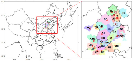
Figure 1.
Simulation domain and observation sites in 2 + 26 cities of North China Plain (red dots: surface monitor sites for NO2, SO2, O3, and PM2.5; the 28 cities are BJ, Beijing; TJ, Tianjin; BD, Baoding; CAZ, Cangzhou; HD, Handan; HS, Hengshui; LF, Langfang; SJZ, Shijiazhuang; TS, Tangshan; XT, Xingtai; TY, Taiyuan; YQ, Yangquan; ZZ, Zhengzhou; JZ, Jiaozuo; AY, Anyang; HB, Hebi; XX, Xinxiang; KF, Kaifeng; PY, Puyang; HZ, Heze; LC, Liaocheng; DZ, Dezhou; JNI, Jining; ZB, Zibo; JNA, Jinan; BZ, Binzhou; JC, Jincheng; CHZ, Changzhi).
The RSM model was developed based on 21 emission-control scenario simulations with the WRF-CMAQ model by implementing polynomial functions to represent the response of O3 and PM2.5 to emission changes of five pollutants including SO2, NOx, VOC, NH3, and pPM2.5 in 28 cities in NCP [14,15]. The polynomial functions of O3 and PM2.5 response to emissions are shown as Equations (1) and (2).
where and are the response of O3 and PM2.5 concentrations (i.e., change to the baseline concentration), respectively, at each simulated grid cell; ENOx, ESO2, ENH3, EVOCs, and EpPM2.5 are the change ratios of NOx, SO2, NH3, VOCs, and pPM2.5 emissions, respectively, relative to baseline (i.e., baseline = 0); is the coefficient of term I, which is determined by fitting with 21 emission-control scenario simulations.
The RSM can predict O3 and PM2.5 responses to emission changes in good agreement with CMAQ predictions, as the out-of-sample validation of RSM predictions against CMAQ simulations yields NMBs (normalized mean biases) within ±1% [28].
We gathered the observed NO2, SO2, O3, and PM2.5 measurements from monitoring sites in the 28 NCP cities from the China National Environmental Monitoring Centre (http://www.cnemc.cn/en/) (Figure 1). The daily maximum 8-hour O3 and daily averaged PM2.5 concentrations were assimilated for the modeling domain with 9-km horizontal grid spacing. The simulation period was January, April, July, and October, 2017 to represent winter, spring, summer, and fall, respectively. The assimilation performance was evaluated using the root mean square error (RMSE), normalized mean bias (NMB), and R-squared (R2).
In the baseline case of RSM-assimilation, we included all observation sites during the assimilation. To compare with the simulation, we averaged observations from sites within the same model grid cell (9 km × 9 km). This resulted in about 85 sites (the number is smaller than that shown in Figure 1) across 28 cities to be used in data assimilation. The monitoring sites were mostly located at the urban center of each city, where both local emission sources and regional contributions influenced the ambient PM2.5 and O3 concentrations [29,30]. The RSM-assimilation can account for both local formation and regional transport since it was original built from CMAQ model simulations. Details about the numbers of sites used for nudging in each city are summarized in Table S1. Additionally, we designed single-site cases for each of the 28 cities in which only a single randomly-selected site was assimilated for each city. These cases were used to examine the sensitivity of the RSM-assimilation method to the number of observation sites.
2.2. RSM-Assimilation Framework
Figure 2 presents the framework for the newly developed RSM-assimilation method. As in our previous study [3], we first estimated the adjusted emission ratios of NOx and SO2 based on the comparison of simulated and observed NO2 and SO2 concentrations. Next, an optimization process was implemented that sampled VOC emission ratios as inputs for the RSM-O3 model. This process resulted in optimized VOC emission ratios for the 28 cities that yielded the best agreement between simulated and observed O3 concentrations at the monitoring sites (determined by the average RMSE over all the sites). A similar optimization process was then applied for PM2.5, where the adjusted NOx, SO2, and VOC emission ratios were introduced into the RSM-PM2.5 model, and emission ratios were sampled for NH3 and pPM2.5 in the 28 cities. Since direct observations of surface NH3 concentrations are unavailable, the optimized pPM2.5 and NH3 emission ratios correspond to the assimilated PM2.5 concentrations that agree most closely with observed PM2.5 concentrations among all possible combinations of emission ratios. The optimization was conducted through a multiple looping process to select the best combination of emission ratios (with a small step of 0.05) for different pollutants and cities to achieve the best overall agreement. As currently designed, the RSM was suitable for emission ratios of gas pollutants that ranged from 0 (fully controlled emissions) to 2 (doubled emissions). The response functions of O3 and PM2.5 to emission changes of gaseous precursors were fitted through the regression of multiple emission-control scenario simulations (emission ratios from 0 to 2); thus, the uncertainties of the response functions will be considerably larger when the emissions vary outside of the 0–2 emission ratio range. Here, we limited the adjusted emission ratios of NO2, SO2, VOC, and NH3 to a range from 0.1 (90% reduction) to 2.0 (100% increase). We allowed a wider range for pPM2.5 emission ratios due to the large uncertainties in pPM2.5 emissions, particularly for fugitive emission sources like wind-blown dust. Unlike the gas pollutants, the RSM had no limits on the adjusted emission ratios for pPM2.5, since the impacts of these emissions were represented linearly in the RSM [16].
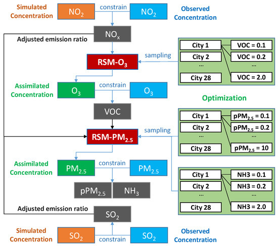
Figure 2.
The emission-concentration-based response modeling framework. (In assimilating observational data, NOx and SO2 emissions were adjusted first, followed by optimization for VOC, and then pPM2.5 and NH3 emissions).
3. Results
3.1. Performance of RSM-Assimilation
In Figure 3 and Figure 4, the assimilated O3 and PM2.5 concentrations in the baseline RSM-assimilation case are compared with the original CMAQ simulations in terms of the spatial pattern of monthly averaged concentrations and with observations in terms of daily paired values for sites in the 28 cities. The assimilated spatial fields generally maintained the spatial distribution of the original CMAQ simulation, but have slightly modulated concentrations in areas surrounding the observation sites that better reflect observed values. The accuracy of both O3 and PM2.5 concentrations was enhanced through the RSM-assimilation that reduced the RMSE from 12.7–24.4 ppb (pre-assimilation) to 9.9–18.1 ppb (post-assimilation) for O3, and from 23.7–85.3 μg·m−3 (pre-assimilation) to 11.8–46.5 μg·m−3 (post-assimilation) for PM2.5.
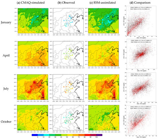
Figure 3.
Comparions of CMAQ-simulated, observed, and RSM-assimilated O3 concentrations: (a) CMAQ-simulation; (b) Observation; (c) RSM-assimilation; (d) Comparison between CMAQ-simulation or RSM-assimilation against with obervation (the comparison was done on a monthly basis for each month of comparison; unit, ppb).
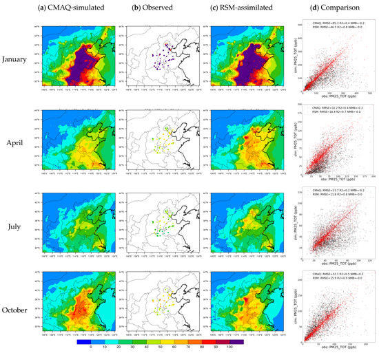
Figure 4.
Comparisons of CMAQ-simulated, observed, and RSM-assimilated PM2.5 concentrations (a) CMAQ-simulation; (b) Observation; (c) RSM-assimilation; (d) Comparison between CMAQ-simulation or RSM-assimilation against with obervation (the comparison was done on a monthly basis for each month of comparison; unit, μg·m−3).
The high biases in simulated O3 were greatly reduced through RSM-assimilation, as the NMBs decrease from up to 50% in CMAQ to within 20% in RSM-assimilation. The underestimation of PM2.5 was also mitigated through RSM-assimilation, as the NMBs for PM2.5 were reduced to 0%. The comparison of daily paired predictions and observations indicated large improvements for R2 in RSM-assimilation: e.g., the R2 for PM2.5 predictions increased from 0.2–0.5 (pre-assimilation) to 0.7–0.9 (post-assimilation). However, the RSM-assimilation was much more effective for PM2.5 than for O3. This behavior might be associated with the large contributions to O3 from sources that cannot be adjusted through RSM assimilation (e.g., biogenic sources) and the effectiveness of primary PM2.5 emissions for modulating PM2.5 concentrations. We note that the observations displayed in Figure 4 are distributed in discrete locations across the domain, and do not necessarily match the location of the simulated and assimilated concentrations (see Figure S2 for the matched location comparisons).
Time-series comparisons for O3 and PM2.5 in the 28 cities (Figure S3 and S4, respectively) suggest similar levels of improvement, as the RMSE was reduced after the four-month assimilation across the 28 cities.
Although the RSM-assimilation improved the simulation accuracy, large discrepancies in the performance improvements were evident among the 28 cities. To further investigate the variation of RSM-assimilation performance across all observation sites, we compared the RMSEs of CMAQ-simulated and RSM-assimilated O3 and PM2.5 in the 28 cities at the four-month averaged level, as shown in Figure 5.
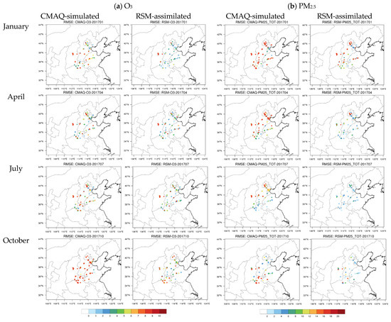
Figure 5.
Comparisons of RMSE in CMAQ-simulated and RSM-assimilated concentrations of O3 (a; unit-ppb) and PM2.5 (b; unit-μg·m−3) across all observation sites.
In general, the RSM-assimilation was less effective in reducing the RMSE for sites in cities at the edge of the control region (i.e., the full 28-city area). The smallest O3 improvements occurred in cities such as ZB on the eastern edge of the control region and YQ on the western edge of the control region. These cities had relatively large RMSEs after the assimilation, with RMSE reductions of only 6% (ZB) and −3% (YQ) (a slightly worse performance) relative to the CMAQ simulation. For the other cities, the O3 improvements were much greater, with RMSE reductions of at least 16%. For PM2.5, YQ also had the smallest improvement, with a 24% reduction in RMSE (compared to a 50–80% for the other cities). Such results indicated that the RSM-assimilation had limited ability to improve the accuracy of concentrations at the edge of the control region, where the influence of emissions from outside of the control region was large. Enlarging the control area or combining it with an RSM model based on the larger domain is recommended to improve the ability of RSM-assimilation for those cities. Meanwhile, discrepancies also existed within a city, e.g., RMSE was reduced in eastern Tianjin but increased in western Tianjin in Jan. This behavior occurred because the RSM-assimilation adjusted emissions at the city averaged level and maintained the spatial distribution of emissions within each city at the a priori estimate. Future improvement of the spatial distribution of the emission within the city is also recommended by adopting additional observations like satellites and advanced technologies like machine-learning to address such limits.
3.2. Sensitivity of RSM-Assimilation to the Site Number
For traditional model-observation fusion methods, the abundance of observations has significant impacts on model performance [8]. However, in RSM-assimilation, the adjustment of emissions is done at the city-level, and therefore decreasing the number of observations within each city should have relatively less influence on performance compared to regression-based methods. To investigate the sensitivity of RSM performance to the number of sites used in the assimilation, we examined performance for cases based on different numbers of observation sites, as shown in Figure 6.
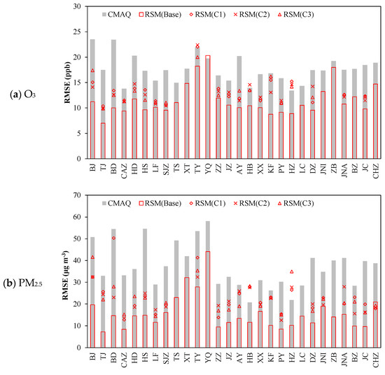
Figure 6.
The performance of RSM-assimilation for O3 (a) and PM2.5 (b) by using a different number of observation sites.
In assimilation for the baseline case (hollow red bar), all observation sites were used. For the other cases (C1 to C3, red symbols), a single site in each city was used based on three random site selections. Compared to the baseline RSM, the performance did not decrease considerably for the single-site RSM-assimilation cases, C1–C3, especially for PM2.5. When the number of observation sites were decreased from 85 to 28, the RMSE in O3 predictions increased slightly (by 13%, from 11.5 to 13.3 ppb) and RMSE in PM2.5 increased slightly (by 42%, from 15.7 to 22.4 μg·m−3) but still decreased by 40% from that in CMAQ (37.3 μg·m−3) based on the average of all 28 cities. We note that the evaluation for C1–C3 was performed while withholding observations from the sites used for assimilation, thus implying that such improvement through assimilation also applies to the locations where air pollution is not monitored.
RSM-assimilation has advantages in cases where few observation data are available. However, since emissions were adjusted at the city level, the RSM-assimilation method has limited flexibility for adjusting spatial patterns of O3 and PM2.5 concentrations. The spatial distribution of emissions, which are assumed to be accurate in RSM-assimilation, might also have uncertainties that could influence the performance of assimilation in terms of representing concentration gradients. In that case, adjustment of total emissions cannot reduce the biases associated with the spatial concentration gradients. This could limit the overall performance of RSM-assimilation.
3.3. Implication of Uncertainties in Anthropogenic Emissions
In addition of reducing the RMSE of model predictions, RSM-assimilation provided the emission ratios for five pollutants that were adjusted simultaneously during assimilation. The adjusted emission ratios provided information about potential uncertainties in anthropogenic emissions.
As shown in Figure 7, for average month values, NOx emissions appear to be underestimated in the baseline case based on emission adjustment ratios > 1 in January, April, and October. VOC emissions appear to be overestimated (adjustment ratios < 1) in January and October, and SO2 emissions are underestimated in April. The emission adjustment ratio for pPM2.5 was the largest among all pollutants, in part due to the wider range of possible changes allowed in the RSM-assimilation. The pPM2.5 ratio was much greater than 1 in all cases and indicated a significant underestimation, particularly in April during the dust season. The biases in assimilated concentrations generally did not reach zero due to the limited range of emission adjustment available in RSM-assimilation. For cases that have large uncertainties in the prior emissions, the simulated concentrations cannot fully be assimilated such that predictions match the observation.
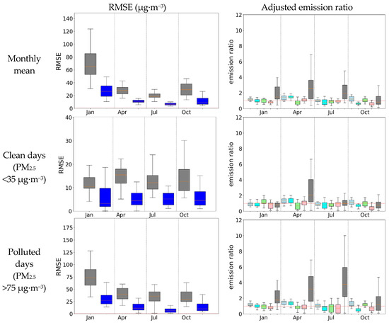
Figure 7.
The RMSE (left: grey, CMAQ; blue, RSM) and Adjusted emission ratio for the air quality assimilation (right: baseline = 1. light blue, NOx; cyan, SO2, green, NH3; pink, VOC; grey, pPM2.5) at different polluted levels.
An underestimation of NOx and SO2 emissions were evident on both clean and polluted days. On clean days, pPM2.5 emissions were significantly underestimated in April. On polluted days, NOx emissions are underestimated during all seasons except summer. For all days, VOC emissions were overestimated in January and October, and SO2 emissions were underestimated in January and April but overestimated in July and October. The adjusted emission ratio for pPM2.5 was greater than 1 across all four months suggesting a broad underestimation of primary PM2.5 emissions. The uncertainties of pPM2.5 emissions may be due to the lack of inline dust simulation over the NCP domain and underestimation of wind-blown dust emissions outside of NCP [31], as such, underestimation of PM2.5 was more pronounced in April during the dust season. Also, the underestimation of primary organic aerosol and intermediate VOC emissions appears to have resulted in relatively larger low-biases of simulated organic aerosols than other components in April (see Figure S5). Although increasing the pPM2.5 emissions is an efficient way to resolve differences between modeled and observed PM2.5 concentrations, the emission adjustment of pPM2.5 also likely corrects for other model limitations. The large adjustment of pPM2.5 (by over two) suggests that other model uncertainties (e.g., aerosol-PBL dynamic interactions, chemical reaction rates, and potential missing chemical reaction pathways) could also play an important role in contributing to low biases. This is also suggested from the evaluation of PM2.5 component concentrations, which imply that potential missing chemical reaction pathways for the transition of S(IV) to S(VI) [32,33] might contribute to the low-biases of sulfate aerosols in January and July (i.e., SO2 concentration was overestimated but the percentage of sulfate aerosols in total PM2.5 was underestimated, see Figure S5). Further decoupling the influence of these processes can be done using advanced machine learning technology with the inclusion of certain feature data such as meteorological variables.
4. Summary and Conclusions
In this study, we developed a new assimilation method (RSM-assimilation) that used an emission-concentration response model for assimilating PM2.5 and O3 observations simultaneously. The successful application of RSM-assimilation indicated that significant improvements in the agreement of predictions and observations could be achieved solely by adjusting the emissions. For instance, the RMSE for O3 and PM2.5 predictions decreased by about 35% and 58%, respectively, demonstrating the effectiveness of the new assimilation method based on the emission-concentration response model. We found that the RSM-assimilation had limited ability for assimilating concentrations at the edge of the control region due to the influence of emissions from surrounding regions. Compared to PM2.5, O3 concentrations were harder to assimilate with the new method due in part to the larger contributions from background and natural sources. An advantage of RSM-assimilation is that it requires very little observational data, since it uses prior knowledge of the spatial distribution of emissions. Therefore the approach is most suitable for cases where few observations are available.
The RSM-assimilation also provides useful information to improve the understanding of uncertainties in the emission inventory. Based on the adjusted emission ratios, we found that the NOx emissions are likely underestimated in January, April, and October; SO2 emissions are likely underestimated in April; NH3 emissions are likely overestimated in April; and VOC emissions are likely overestimated in January and October. Also, pPM2.5 emissions appear to be significantly underestimated in April during the dust season. Despite the success of the RSM-assimilation application, some limitations were identified that require future improvement. For example, due to the lack of NH3 observations, we adjusted the NH3 emissions simultaneously with pPM2.5 emissions in this study. Future work can be conducted by implementing both surface measurements and satellite retrievals (e.g., NO2, SO2, NH3, and HCHO) to optimize the emission accuracy across the whole domain. The inclusion of NH3 observations can improve the method to better constrain the adjustment for PM2.5. Further improvement can be also done to separate the emissions by sectors, with additional correction functions such as the spatial pattern of each emission category based on observations like satellites. In addition, we assumed that the emission changes have an immediate impact on PM2.5 and O3 concentrations, but incorporating an assimilation time window into the method is necessary to account for the time needed for pollution transport and chemical formation upwind of the monitors.
Supplementary Materials
The following are available online at https://www.mdpi.com/2073-4433/11/12/1289/s1, Table S1: number of sites used for nudging in each city, Figure S1: Spatial distribution of five air pollutants emissions of 28 cities in NCP (unit, kt·grid−1·yr−1), Figure S2: Comparisons of CMAQ-simulated, observed, and RSM-assimilated PM2.5 concentrations in Apr 2017, Figure S3: Comparison of observed, CMAQ-simulated, and RSM-assimilated O3 concentration, Figure S4: Comparison of observed, CMAQ-simulated and RSM-assimilated PM2.5 concentration, Figure S5: Comparison of observed and simulated PM2.5 chemical component in a Beijing urban site (relative percentage in total PM2.5 mass concentration).
Author Contributions
Conceptualization, methodology, validation, formal analysis, and original draft preparation—J.X. and S.L.; resources, D.D. and Y.Z.; data curation, S.W.; writing—review and editing, J.T.K.; supervision, project administration, and funding acquisition, S.W., C.J., and J.H.; All authors have read and agreed to the published version of the manuscript.
Funding
This work was supported in part by the National Key R&D program of China (2017YFC0213005) and the National Natural Science Foundation of China (41907190, 51861135102). This work was completed on the “Explorer 100” cluster system of the Tsinghua National Laboratory for Information Science and Technology.
Acknowledgments
The authors gratefully acknowledge the free availability and use of observation datasets. The views expressed in this manuscript are those of the authors alone and do not necessarily reflect the views and policies of the US Environmental Protection Agency.
Conflicts of Interest
The authors declare no conflict of interest. The funders had no role in the design of the study; in the collection, analyses, or interpretation of data; in the writing of the manuscript, or in the decision to publish the results.
Abbreviations
| CMAQ model | community multiscale air quality model |
| CTM | chemical transport model |
| DS | downscaler |
| eVNA | enhanced Voronoi neighbor averaging |
| HCHO | formaldehyde |
| MEGAN | model for emissions of gases and aerosols from nature |
| MEIC | multi-resolution emission inventory for China |
| NCP | North China Plain |
| NH3 | ammonia |
| NMB | normalized mean bias |
| NOx | nitrogen oxides |
| O3 | ozone |
| PBL | planetary boundary layer |
| PM2.5 | fine particulate matter |
| pPM2.5 | primary fine particulate matter |
| R2 | R-squared |
| RMSE | root mean square error |
| RSM | response surface model |
| SO2 | sulfur dioxide |
| VNA | Voronoi neighbor averaging |
| VOC | volatile organic compounds |
| WRF model | weather research and forecasting model |
References
- Forouzanfar, M.H.; Alexander, L.W.G.; Anderson, H.R.; Bachman, V.F.; Biryukov, S.; Brauer, M.; Burnett, R.T.; Casey, D.; Coates, M.M.; Cohen, A.; et al. Global, regional, and national comparative risk assessment of 79 behavioural, environmental and occupational, and metabolic risks or clusters of risks in 188 countries, 1990–2013: A systematic analysis for the Global Burden of Disease Study 2013. Lancet 2015, 386, 2287–2323. [Google Scholar] [CrossRef]
- Health Effects Institute. State of Global Air 2019. Available online: www.stateofglobalair.org (accessed on 22 August 2019).
- Xing, J.; Li, S.; Jiang, Y.; Wang, S.; Ding, D.; Dong, Z.; Zhu, Y.; Hao, J. Quantifying the emission changes and associated air quality impacts during the COVID-19 pandemic in North China Plain: A response modeling study. Atmos. Chem. Phys. 2020, 20, 14347–14359. [Google Scholar] [CrossRef]
- Gold, C.M.; Remmele, P.R.; Roos, T. Voronoi methods in GIS. In Algorithmic Foundations of Geographic Information Systems. Lecture Notes in Computer Science; van Kreveld, M., Nievergelt, J., Roos, T., Widmayer, P., Eds.; Springer: Berlin/Heidelberg, Germany, 1997; pp. 21–35. [Google Scholar]
- Ding, D.; Zhu, Y.; Jang, C.; Lin, C.-J.; Wang, S.; Fu, J.; Gao, J.; Deng, S.; Xie, J.; Qiu, X. Evaluation of health benefit using BenMAP-CE with an integrated scheme of model and monitor data during Guangzhou Asian Games. J. Environ. Sci. 2016, 42, 9–18. [Google Scholar] [CrossRef] [PubMed]
- U.S. EPA. Bayesian Space-Time Downscaling Fusion Model (Downscaler) Derived Estimates of Air Quality for 2017; U.S. Environmental Protection Agency: Washington, DC, USA, 2020. Available online: https://nepis.epa.gov (accessed on 29 November 2020).
- U.S. EPA. Technical Information about Fused Air Quality Surface Using Downscaling Tool: Metadata Description; U.S. Environmental Protection Agency: Washington, DC, USA, 2016. Available online: https://www.epa.gov/air-research/technical-information-about-fused-air-quality-surface-using-downscaling-tool (accessed on 29 November 2020).
- Li, J.; Zhu, Y.; Kelly, J.T.; Jang, C.J.; Wang, S.; Hanna, A.; Xing, J.; Lin, C.-J.; Long, S.; Yu, L. Health benefit assessment of PM2.5 reduction in Pearl River Delta region of China using a model-monitor data fusion approach. J. Environ. Manag. 2019, 233, 489–498. [Google Scholar] [CrossRef] [PubMed]
- Kelly, J.T.; Jang, C.J.; Timin, B.; Gantt, B.; Reff, A.; Zhu, Y.; Long, S.; Hanna, A. A system for developing and projecting PM2.5 spatial fields to correspond to just meeting national ambient air quality standards. Atmos. Environ. X 2019, 2, 100019. [Google Scholar] [CrossRef]
- Lu, X.; Zhang, S.; Xing, J.; Wang, Y.; Chen, W.; Ding, D.; Wu, Y.; Wang, S.; Duan, L.; Hao, J. Progress of Air Pollution Control in China and Its Challenges and Opportunities in the Ecological Civilization Era. Engineering 2020. [Google Scholar] [CrossRef]
- Mendoza, A.; Russell, A.G. Iterative Inverse Modeling and Direct Sensitivity Analysis of a Photochemical Air Quality Model. Environ. Sci. Technol. 2000, 34, 4974–4981. [Google Scholar] [CrossRef]
- Miyazaki, K.; Eskes, H.; Sudo, K.; Boersma, K.F.; Bowman, K.; Kanaya, Y. Decadal changes in global surface NOx emissions from multi-constituent satellite data assimilation. Atmos. Chem. Phys. Discuss. 2017, 17, 807–837. [Google Scholar] [CrossRef]
- Tang, W.; Cohan, D.S.; Lamsal, L.N.; Xiao, X.; Zhou, W. Inverse modeling of Texas NOx emissions using space-based and ground-based NO2 observations. Atmos. Chem. Phys. Discuss. 2013, 13, 11005–11018. [Google Scholar] [CrossRef]
- Zhang, L.; Chen, Y.; Zhao, Y.; Henze, D.K.; Zhu, L.; Song, Y.; Paulot, F.; Liu, X.; Pan, Y.; Lin, Y.; et al. Agricultural ammonia emissions in China: Reconciling bottom-up and top-down estimates. Atmos. Chem. Phys. Discuss. 2018, 18, 339–355. [Google Scholar] [CrossRef]
- Xing, J.; Wang, S.-X.; Zhao, B.; Wu, W.; Ding, D.; Jang, C.; Zhu, Y.; Chang, X.; Wang, J.; Zhang, F.; et al. Quantifying Nonlinear Multiregional Contributions to Ozone and Fine Particles Using an Updated Response Surface Modeling Technique. Environ. Sci. Technol. 2017, 51, 11788–11798. [Google Scholar] [CrossRef] [PubMed]
- Xing, J.; Ding, D.; Wang, S.; Zhao, B.; Jang, C.; Wu, W.; Zhang, F.; Zhu, Y.; Hao, J. Quantification of the enhanced effectiveness of NO x control from simultaneous reductions of VOC and NH 3 for reducing air pollution in the Beijing–Tianjin–Hebei region, China. Atmos. Chem. Phys. 2018, 18, 7799–7814. [Google Scholar] [CrossRef]
- Xing, J.; Zheng, S.; Ding, D.; Kelly, J.T.; Wang, S.; Li, S.; Qin, T.; Ma, M.; Dong, Z.; Jang, C.J.; et al. Deep Learning for Prediction of the Air Quality Response to Emission Changes. Environ. Sci. Technol. 2020, 54, 8589–8600. [Google Scholar] [CrossRef] [PubMed]
- Ding, D.; Xing, J.; Wang, S.; Liu, K.; Hao, J. Estimated Contributions of Emissions Controls, Meteorological Factors, Population Growth, and Changes in Baseline Mortality to Reductions in Ambient PM2.5 and PM2.5-Related Mortality in China, 2013–2017. Environ. Health Perspect. 2019, 127, 067009. [Google Scholar] [CrossRef]
- Morrison, H.; Thompson, G.; Tatarskii, V. Impact of Cloud Microphysics on the Development of Trailing Stratiform Precipitation in a Simulated Squall Line: Comparison of One- and Two-Moment Schemes. Mon. Weather Rev. 2009, 137, 991–1007. [Google Scholar] [CrossRef]
- Iacono, M.J.; Delamere, J.S.; Mlawer, E.J.; Shephard, M.W.; Clough, S.A.; Collins, W.D. Radiative forcing by long-lived greenhouse gases: Calculations with the AER radiative transfer models. J. Geophys. Res. Space Phys. 2008, 113, 113. [Google Scholar] [CrossRef]
- Kain, J.S. The kain-fritsch convective parameterization: An update. J. Appl. Meteorol. 2004, 43, 170–181. [Google Scholar] [CrossRef]
- Xiu, A.; Pleim, J.E. Development of a Land Surface Model. Part I: Application in a Mesoscale Meteorological Model. J. Appl. Meteorol. 2001, 40, 192–209. [Google Scholar] [CrossRef]
- Pleim, J.E. A Combined Local and Nonlocal Closure Model for the Atmospheric Boundary Layer. Part I: Model Description and Testing. J. Appl. Meteorol. Clim. 2007, 46, 1383–1395. [Google Scholar] [CrossRef]
- Sarwar, G.; Luecken, D.; Yarwood, G.; Whitten, G.Z.; Carter, W.P.L. Impact of an Updated Carbon Bond Mechanism on Predictions from the CMAQ Modeling System: Preliminary Assessment. J. Appl. Meteorol. Clim. 2008, 47, 3–14. [Google Scholar] [CrossRef]
- Appel, K.W.; Pouliot, G.; Simon, H.; Sarwar, G.; Pye, H.O.T.; Napelenok, S.L.; Akhtar, F.; Roselle, S.J. Evaluation of dust and trace metal estimates from the Community Multiscale Air Quality (CMAQ) model version 5.0. Geosci. Model Dev. 2013, 6, 883–899. [Google Scholar] [CrossRef]
- Li, M.; Zhang, Y.; Kurokawa, J.-I.; Woo, J.-H.; He, K.; Lu, Z.; Ohara, T.; Song, Y.; Streets, D.G.; Carmichael, G.R.; et al. MIX: A mosaic Asian anthropogenic emission inventory under the international collaboration framework of the MICS-Asia and HTAP. Atmos. Chem. Phys. 2017, 17, 935–963. [Google Scholar] [CrossRef]
- Guenther, A.; Karl, T.; Harley, P.; Wiedinmyer, C.; Palmer, P.I.; Geron, C. Estimates of global terrestrial isoprene emissions using MEGAN (Model of Emissions of Gases and Aerosols from Nature). Atmos. Chem. Phys. Discuss. 2006, 6, 3181–3210. [Google Scholar] [CrossRef]
- Ding, D. Response Surface Model of Atmospheric PM2.5 and O3 Concentration with Precursor Emissions and Its Application. Ph.D Thesis, Tsinghua University, Beijing, China, 2020. [Google Scholar]
- Chang, X.; Wang, S.; Zhao, B.; Xing, J.; Liu, X.; Wei, L.; Song, Y.; Wu, W.; Cai, S.; Zheng, H.; et al. Contributions of inter-city and regional transport to PM2.5 concentrations in the Beijing-Tianjin-Hebei region and its implications on regional joint air pollution control. Sci. Total Environ. 2019, 660, 1191–1200. [Google Scholar] [CrossRef]
- Dong, Z.; Wang, S.; Xing, J.; Chang, X.; Ding, D.; Zheng, H. Regional transport in Beijing-Tianjin-Hebei region and its changes during 2014–2017: The impacts of meteorology and emission reduction. Sci. Total Environ. 2020, 737, 139792. [Google Scholar] [CrossRef]
- Xing, J.; Mathur, R.; Pleim, J.; Hogrefe, C.; Gan, C.-M.; Wong, D.C.; Wei, C. Can a coupled meteorology–chemistry model reproduce the historical trend in aerosol direct radiative effects over the Northern Hemisphere? Atmos. Chem. Phys. 2015, 15, 9997–10018. [Google Scholar] [CrossRef]
- Fu, X.; Wang, S.; Chang, X.; Cai, S.; Xing, J.; Hao, J. Modeling analysis of secondary inorganic aerosols over China: Pollution characteristics, and meteorological and dust impacts. Sci. Rep. 2016, 6, 35992. [Google Scholar] [CrossRef]
- Zhang, S.; Xing, J.; Sarwar, G.; Ge, Y.; He, H.; Duan, F.K.; Zhao, Y.; He, K.; Zhu, L.; Chu, B. Parameterization of heterogeneous reaction of SO2 to sulfate on dust with coexistence of NH3 and NO2 under different humidity conditions. Atmos. Environ. 2019, 208, 133–140. [Google Scholar] [CrossRef]


Publisher’s Note: MDPI stays neutral with regard to jurisdictional claims in published maps and institutional affiliations. |
© 2020 by the authors. Licensee MDPI, Basel, Switzerland. This article is an open access article distributed under the terms and conditions of the Creative Commons Attribution (CC BY) license (http://creativecommons.org/licenses/by/4.0/).