The Energy, Momentum, and Peak Power Radiated by Negative Lightning Return Strokes

Abstract

Electromagnetic radiation fields generated by return strokes transport both energy and momentum from the return stroke to outer space. The momentum transported by the radiation field has only a vertical or z component due to azimuthal symmetry (cylindrical symmetry) associated with a vertical return stroke. In this paper, the energy, momentum, and peak power radiated by return strokes as a function of the return stroke current, return stroke speed, and the zero-crossing time of the radiation fields are studied. The results obtained by numerical simulations for the energy, vertical momentum, and the peak power radiated by lightning return strokes (all parameters normalized by dividing them by the square of the radiation field peak at 100 km) are the following: A typical first return stroke generating a radiation field having a 50 μs zero-crossing time will dissipate field normalized energy of about (1.7–2.5) × 10³ J/(V/m)² and field-normalized vertical momentum of approximately (2.3–3.1) × 10⁻⁶ Kg m/s/(V/m)². A radiation field with a zero-crossing time of 70 μs will dissipate about (2.6–3.4) × 10³ J/(V/m)² in field-normalized energy and (3.2–4.3) × 10⁻⁶ Kg m/s/(V/m)² in field-normalized vertical momentum. The results show that, for a given peak radiation field, the radiated energy and momentum increase with increasing zero-crossing time of the radiation field. The normalized peak power generated by a first return stroke radiation field is about 1.2 × 10⁸ W/(V/m)² and the peak power is generated within about 5–6 μs from the beginning of the return stroke. Conversely, a typical subsequent return stroke generating a radiation field having a 40 μs zero-crossing time will dissipate field-normalized energy of about (6–9) × 10² J/(V/m)² and field-normalized vertical momentum of approximately (7.5–11) × 10⁻⁷ Kg m/s/(V/m)². The field-normalized peak power generated by a subsequent return stroke radiation field is about 1.26 × 10⁸ W/(V/m)² and the peak power is generated within about 0.7–0.8 μs from the beginning of the return stroke. In addition to these parameters, the possible upper bounds for the energy and momentum radiated by return strokes are also presented.

1. Introduction

Electromagnetic fields generated by lightning play an essential role in lightning protection studies since they generate unwanted currents and voltages in electrical and electronic systems, causing them damage and disruptions [1]. They can be utilized as a vehicle to study the terrain features by analyzing how these fields are modified when they travel along grounds of different configurations and electrical properties [2,3,4]. These fields can also be used in remote sensing of the spatial and temporal distribution of lightning currents by appealing to different types of return stroke models [5]. Moreover, upper atmospheric physicists also need information concerning electromagnetic fields generated by lightning because these fields interact with the upper atmosphere generating electrical discharge activity such as sprites and elves [6]. Electromagnetic fields from lightning can also modify the temperature of the electrons in the ionosphere and therefore, could change the electromagnetic propagation characteristics of the ionosphere [7]. The energy transported by the electromagnetic fields plays a significant role in many of these interactions. Moreover, in physics-based return stroke models, the knowledge concerning the fraction of energy removed from the lightning channel by electromagnetic radiation is an essential parameter in evaluating the energy balance of the lightning return stroke [5].

Taylor and Jean [8] conducted the first study on the electromagnetic energy radiated by lightning flashes. Using typical features of atmospherics (i.e., distant radiation fields) generated by return strokes, they estimated that a return stroke would dissipate about 3 × 10⁴ J on average as electromagnetic radiation. Taylor [9] improved the results of the study by using a large sample of atmospherics and came up with 7 × 10⁴ J as a typical value for the radiated energy. Recently, armed with more recent data pertinent to electromagnetic fields from return strokes, Krider and Guo [10] estimated that the peak power radiated by typical first and subsequent return strokes to be about (1–2) × 10¹⁰ W and (3–5) × 10⁹ W, respectively. In determining the power and energy dissipated by return strokes utilizing the measured electromagnetic fields, both Taylor [9] and Krider and Guo [10] represented the return stroke as an infinitesimal dipole at ground level with a suitable current moment that reproduced the measured electromagnetic field at ground level. Using this current moment in the dipole, they estimated the Poynting vector at any given point in space. The energy and peak power are estimated by integrating the resulting Poynting vector over the surface of a hemisphere with the center at the strike point. Now, replacing the return stroke as a dipole at ground level will simplify the evaluation of the radiated power and energy from the lightning return stroke. Still, it will introduce errors because the return stroke is an extended source through which current pulses are propagating with speeds close to the speed of light. For example, in the dipole approximation, the temporal variation of the electromagnetic radiation fields is independent of the elevation angle of the point of observation with respect to the vertical, while in an extended source, the duration of the electromagnetic field at different elevation angles depends on the propagation speed of the return stroke; this could influence the calculated energy.

Krider [11] improved the energy calculation by utilizing electromagnetic fields pertinent to the transmission line model [12] to derive an expression for the Poynting vector. From this expression, he estimated the angular distribution of the electromagnetic power radiated by lightning. However, the study has not assessed the total energy radiated out by a return stroke. It is important to point out here, that in the transmission line model, the return stroke current is assumed to propagate with constant speed without attenuation. In reality, the current attenuates, and the speed decreases as the return stroke front forge along the return stroke channel. Both these effects could affect the power and energy radiated by return strokes.

The energy dissipated by a return stroke radiation field depends on its initial peak amplitude, which is related to the return stroke peak current, and on its duration. The duration of the radiation field varies from one return stroke to another, and the zero-crossing time of a radiation field is a good measure of this duration. The zero-crossing time of first return stroke radiation fields may vary from 50 μs in the temperate regions to about 90 μs in the tropics [13]. In the case of subsequent return strokes, it may vary from about 20 μs to about 60 μs. The goal of this work is to examine how the energy, momentum, and peak power radiated by return stroke radiation fields vary with these parameters. Neither the momentum transported by the lightning electromagnetic fields nor the dependence of radiated energy and momentum on the zero-crossing time of the radiation field has ever been studied previously in the literature. But, this information is valuable in understanding the coupling of the lightning generated electromagnetic fields to the upper atmosphere. This paper is an attempt to fill this gap in the literature.

It is vital to point out here that even for a given initial peak and the zero-crossing time of the radiation field, the radiated energy and momentum may depend on the details of the temporal variation of the return stroke radiation field. The temporal variation of the radiation field may also vary from one return stroke to another. To take this variation into account, in our analysis we will use two types of return stroke models that produce different wave shapes for the radiation fields. The two models provide return stroke radiation fields that differ from each other, and we believe that use of these two models will allow us to obtain more information on how the energy and momentum radiated by these fields vary with the shape of the radiation fields.

In this paper, we will use the term range-normalized electric radiation field to represent the peak value of the electric radiation field corresponding to 100 km distance. In describing the results, we will also use the terms field-normalized energy, field-normalized momentum, and field-normalized power. These quantities are generated by dividing the energy, momentum, and power by the square of the electric radiation field peak at 100 km.

Preliminary results of this paper were presented at the 34th International Conference on Lightning Protection (ICLP) held in Rzeszow, Poland, in 2018 [14].

2. Lightning Return Stroke Model Used in the Study

It is necessary to appeal to a return stroke model that specifies the spatial and temporal variation of the return stroke current to calculate the electromagnetic fields from lightning return strokes. However, as we will show later, the energy transported by return stroke radiation fields depends on the shape, amplitude, and duration of the radiation fields. The features of the radiation fields predicted by different models may vary significantly. In the present study, we estimated the energy and momentum transported by return stroke radiation fields as predicted by two return stroke models that belong to the Modified Transmission Line (MTL) type models to identify the effects of these variations on the energy and momentum transported by return strokes. These are the MTL model with exponential current decay (MTLE) and the MTL model with linear current decay (MTLL) [15,16]. According to MTLE and MTLL models, the current distribution along the return stroke channel is given by

$$I(t,z)=I_b(t-z/v)A(z)\mathrm{for}t\ge z/v$$

(1)

$$I(t,z)=0\mathrm{for}t<z/v$$

(2)

In the MTLE model, $A(z)=e^{-z/\lambda }$, and in the MTLL model, $A(z)=(1-z/H)$, where $\lambda$ is the current decay height constant and $H$ is the height of the return stroke channel. In the mathematical expressions given above, $z$ is the vertical coordinate or the height along the return stroke channel, $I_b(t,z)$ is the return stroke current at the channel base and $v$ is the return stroke speed. Now, as mentioned previously, in addition to the initial peak, the duration of the radiation field is a parameter that influences the amount of energy and momentum radiated by return strokes. The zero-crossing time of the radiation field is a measure of its duration. For this reason, we present the results for the radiated energy and momentum as a function of the zero-crossing time and the initial peak of radiation fields. Such a presentation allows comparing the predictions of different return stroke models on radiated energy and momentum. Moreover, the peak and the zero-crossing time of the radiation fields of the return strokes can be measured in practice, and this permits us to extrapolate the results presented here to the actual return strokes using peak amplitude and zero-crossings as measures.

The current waveform used in the present study to represent the channel base current of first and subsequent return strokes is given by [17].

$$i(t)=i_{01}\frac{{(t/{\tau }_{11})}^2}{{(t/{\tau }_{11})}^2+1}{e}^{-t/{\tau }_{21}}+i_{02}\frac{{(t/{\tau }_{12})}^2}{{(t/{\tau }_{12})}^2+1}{e}^{-t/{\tau }_{22}}$$

(3)

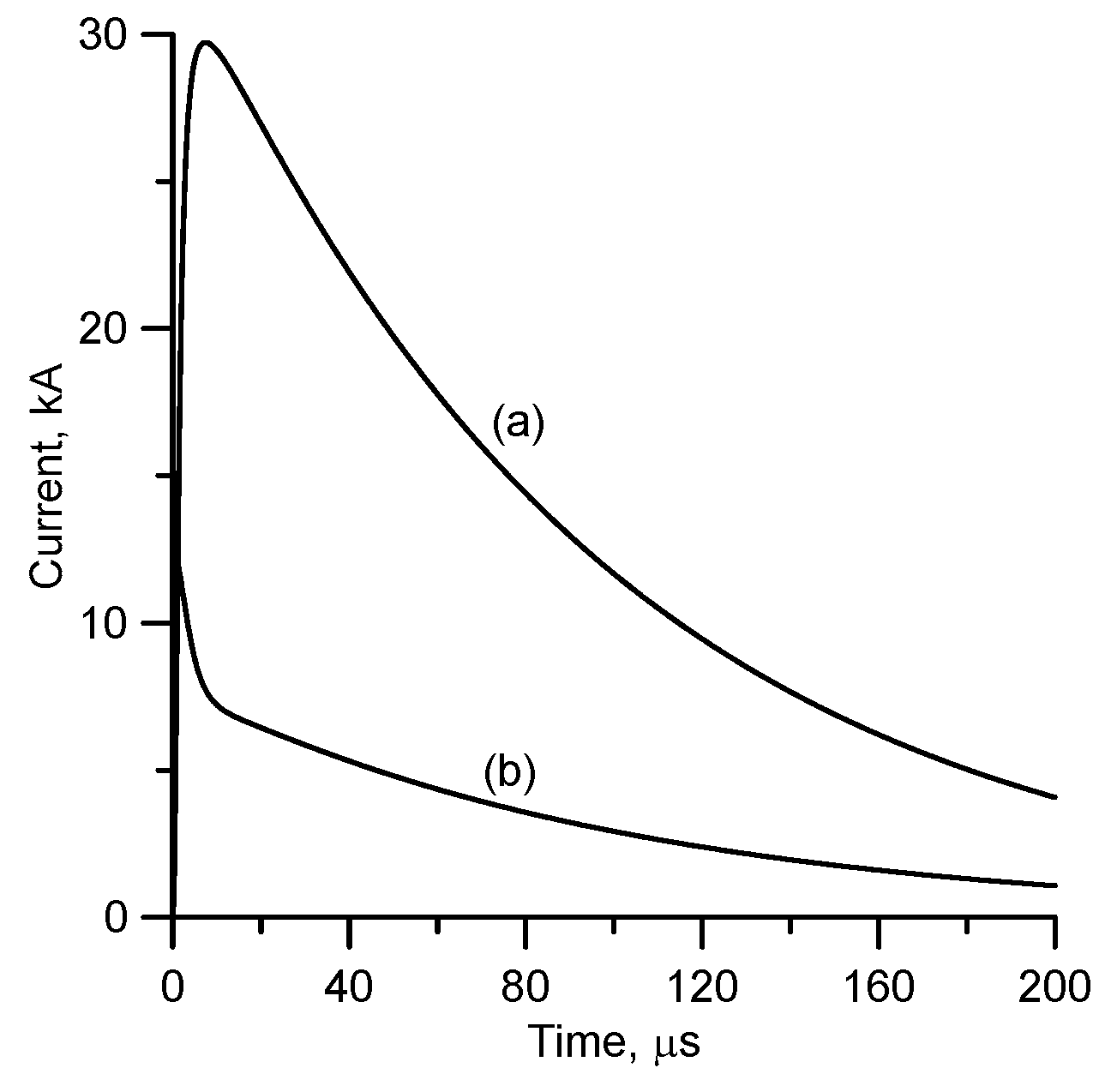
The parameters of this equation for the subsequent return strokes are $i_{01}$ = 10.7 kA, ${\tau }_{11}$ = 0.25 μs, ${\tau }_{21}$ = 2.5 μs, $i_{02}$ = 6.5 kA, ${\tau }_{12}$ = 2.0 μs, and ${\tau }_{22}$ = 100 μs. The first return stroke is represented using only the first term in Equation 3 with parameters $i_{01}$ = 28 kA, ${\tau }_{11}$ = 1.5 μs, and ${\tau }_{21}$ = 95 μs. Figure 1 depicts these current waveforms. Observe that the individual parameters in the above expression for the current cannot be connected individually to the physical current parameters such as the peak current and current risetime. However, the combination of these parameters gives rise to current waveforms that are in reasonable agreement with observations.

3. Electromagnetic Fields from the Lightning Channel

Figure 2 illustrates the geometrical parameters necessary to describe the electric field and the magnetic field intensity. Let us represent the lightning channel by a straight vertical channel located over a perfectly conducting ground plane. In calculating electric and magnetic fields, an image channel replaces the perfectly conducting ground. Consider an infinitesimal channel element of length $dz$ located at height $z$ along the channel. The electric and magnetic fields generated by this current element at point P is given by [18,19].

$$e_{r_1}(t,r_1,{\theta }_1)=\frac{dz}{2\pi {\epsilon }_0}\cos {\theta }_1\left[\frac{1}{c{r}_1^2}I(t-r_1/c,z)+\frac{1}{r_1^3}{\displaystyle \underset{t-r_1/c}{\overset{t}{\int }}I(\tau ,z)d\tau }\right]a_{r_1}$$

(4)

$$e_{{\theta }_1}(t,r_1,{\theta }_1)=\frac{dz}{4\pi {\epsilon }_0}\sin {\theta }_1\left[\frac{1}{c^2{r}_1}\frac{\partial I(t-r_1/c,z)}{\partial t}+\frac{1}{c{r}_1^2}I(t-r_1/c,z)+\frac{1}{r_1^3}{\displaystyle \underset{t-r_1/c}{\overset{t}{\int }}I(\tau ,z)d\tau }\right]a_{{\theta }_1}$$

(5)

$$h_{\phi r}(t,r_1,{\theta }_1)=\frac{dz}{4\pi }\sin {\theta }_1\left[\frac{1}{c{r}_1}\frac{\partial I(t-r_1/c,z)}{\partial t}+\frac{I(t-r_1/c,z)}{r_1^2}\right]a_{\phi }$$

(6)

The resulting fields due to the image current in the perfectly conducting ground plane is given by

$$e_{r_2}(t,r_2,{\theta }_2)=\frac{dz}{2\pi {\epsilon }_0}\cos {\theta }_2\left[\frac{1}{c{r}_2^2}I(t-r_2/c,z)+\frac{1}{r_2^3}{\displaystyle \underset{t-r_2/c}{\overset{t}{\int }}I(\tau ,z)d\tau }\right]a_{r_2}$$

(7)

$$e_{{\theta }_2}(t,r_2,{\theta }_2)=\frac{dz}{4\pi {\epsilon }_0}\sin {\theta }_2\left[\frac{1}{c^2{r}_2}\frac{\partial I(t-r_2/c,z)}{\partial t}+\frac{1}{c{r}_2^2}I(t-r_2/c,z)+\frac{1}{r_2^3}{\displaystyle \underset{t-r_2/c}{\overset{t}{\int }}I(\tau ,z)d\tau }\right]a_{{\theta }_2}$$

(8)

$$h_{\phi i}(t,r_2,{\theta }_2)=\frac{dz}{4\pi }\sin {\theta }_2\left[\frac{1}{c{r}_2}\frac{\partial I(t-r_2/c,z)}{\partial t}+\frac{I(t-r_2/c,z)}{r_2^2}\right]a_{\phi }$$

(9)

Observe that the field components given above are the time domain electric and magnetic fields of a small current element of length dz that contain 1/r, 1/r², and 1/r³ terms. The components of the electric field in the direction of unit vectors $a_r$ and $a_{\theta }$ are then given by

$$e_r(t,r,\theta )=\left[e_{r_1}·a_r+e_{{\theta }_1}·a_r+e_{r_2}·a_r+e_{{\theta }_2}·a_r)\right]a_r$$

(10)

$$e_{\theta }(t,r,\theta )=\left[e_{r_1}·a_{\theta }+e_{{\theta }_1}·a_{\theta }+e_{r_2}·a_{\theta }+e_{{\theta }_2}·a_{\theta }\right]a_{\theta }$$

(11)

The total electric radiation fields in $a_r$ and $a_{\theta }$ directions and the total magnetic radiation field intensity in the $a_{\phi }$ direction can be obtained by summing up the contributions to these field components from all channel elements located along the return stroke channel including the image in the perfectly conducting ground. That is:

$$E_r(t,r,\theta )={\displaystyle \underset{0}{\overset{H}{\int }}{e}_r}(t,r,\theta )dz$$

(12)

$$E_{\theta }(t,r,\theta )={\displaystyle \underset{0}{\overset{H}{\int }}{e}_{\theta }}(t,r,\theta )dz$$

(13)

$$H_{\phi }(t,r,\theta )={\displaystyle \underset{0}{\overset{H}{\int }}\left\{h_{\phi r}(t,r_1,{\theta }_1)+h_{\phi i}(t,r_2,{\theta }_2)\right\}}dz$$

(14)

Note that due to azimuthal (or cylindrical) symmetry, the fields are independent of the azimuth angle $\phi$.

4. Expressions for the Power, Energy, and Momentum of the Electromagnetic Fields

The Poynting vector, $S(t,\theta ,r)$, which is directed along the vector $a_r$, associated with the fields, is given by

$$S(t,r,\theta )=E_{\theta }(t,r,\theta )\times H_{\phi }(t,r,\theta )$$

(15)

This Poynting vector can be utilized to obtain the power $P(t)$, energy $U$, flux of momentum in the z-direction $M_z(t)$ and the total momentum transferred along the z-direction $M_{zT}$ as follows [18,19]:

$$P(t)={\displaystyle \underset{\phi =0}{\overset{2\pi }{\int }}{\displaystyle \underset{\theta =0}{\overset{\pi /2}{\int }}S(t,r,\theta )r^2\sin \theta \hspace{0.17em}d\theta \hspace{0.17em}d\phi }}$$

(16)

$$U={\displaystyle \underset{0}{\overset{T}{\int }}P(t)dt}$$

(17)

$$M_z(t)=\frac{1}{c}{\displaystyle \underset{\phi =0}{\overset{2\pi }{\int }}{\displaystyle \underset{\theta =0}{\overset{\pi /2}{\int }}S(t,r,\theta )r^2\sin \theta \cos \theta \hspace{0.17em}d\theta \hspace{0.17em}d\phi }}$$

(18)

$$M_{zT}={\displaystyle \underset{0}{\overset{T}{\int }}{M}_z(t)dt}$$

(19)

Note that the momentum has a component only in the z-direction due to symmetry.

It is worthy to point out here that at sufficiently large distances (exact distance depends on the frequency content of the channel base current and the return stroke height), the electric and magnetic fields become pure radiation. In this case, Equations (16)–(19) define the power, energy, and momentum radiated away by the return stroke. At shorter distances, the electromagnetic field terms varying as $1/r^2$ and $1/r^3$ also contribute to the radial Poynting vector. As we show later, these contributions represent the energy transferred between the source and the nearby space, and vice versa.

5. Results

One can deduce from the equations given in the previous section, that for a given current wave shape, the energy, momentum, and the peak power radiated by a return stroke is proportional to the square of the peak of the return stroke current. For this reason, the results are obtained only for 12 kA peak current for the subsequent strokes and 30 kA peak current for the first strokes. Using the proportionality as mentioned above, one can easily obtain the amount of energy, momentum, or peak power radiated by return strokes having other values of peak currents. However, these parameters, especially the energy and momentum, depend not only on the return stroke peak current but also on how the temporal features of the radiation fields vary at different elevations on the surface of a hemisphere centered at the point of the strike of the return stroke. For this reason, first, we will illustrate how the return stroke radiation field varies as a function of the elevation angle $\theta$.

5.1. Radiation Field at Different Elevation Angles

Consider a hemisphere of radius $R$ with the center at the point of strike of the return stroke. The hemisphere lies in the upper half-space of Figure 2, i.e., above the ground. Let us select the distance $R$ such that the fields at that distance are pure radiation. Consider a cross-section of this hemisphere along the z-x plane. As one moves along this cross-section of the hemisphere, the radial distance to the point of strike remains constant at $R$ while the angle $\theta$ varies. The angle $\theta$ is equal to $\pi /2$ at ground level, and $\theta =0$ directly above the strike point. We will present how the radiation field varies with an angle $\theta$ using the radiation fields of subsequent return strokes of the MTLL model.

Figure 3 depicts the radiation fields of subsequent return stroke at two different elevation angles (90° and 20°) and for two different return stroke speeds (1.5 × 10⁸ m/s and 2.5 × 10⁸ m/s) at 100 km distance from the strike point. The results are based on the MTLL model and we have selected the parameter H in such a way that the radiation fields at ground level (i.e., $\theta$ = 90°) for the two return stroke speeds have the same temporal variation (i.e., H = 3730 m for $v$ = 1.5 × 10⁸ m/s and H = 9260 m for $v$ = 2.5 × 10⁸ m/s respectively). Observe from Equations (5), (6), (8) and (9) that the radiation field is proportional to the $\sin \theta$ (note that at large distances, $\sin {\theta }_1=\sin {\theta }_2=\sin \theta$). Thus, the amplitude of the radiation field decreases as $\theta$ decreases. In the waveforms presented in Figure 3, this dependency is removed by normalizing the amplitude of all the electric fields to unity. Note how the radiation field becomes narrower as the angle of elevation decreases. Indeed, this effect depends on the speed of propagation of the return stroke. As the speed increases the radiation fields become narrower with decreasing angle of elevation (i.e., angle $\theta$).

5.2. Energy and Momentum Radiated by Return Strokes

As mentioned previously, the energy and momentum radiated by return strokes depend also on the duration of the radiation field, and the zero-crossing time can act as a measure of this duration. In general, the zero-crossing time of the radiation field depends on the duration of the return stroke current, how the return stroke current is attenuated along the channel, return stroke speed, and the return stroke channel length [20]. In the MTLL and MTLE models, once the channel base current is specified, the zero-crossing time of the radiation field is controlled by the return stroke speed, and how the return stroke current is attenuated along the channel as specified by the parameters $H$ and $\lambda$, in the MTLL and MTLE models respectively. In obtaining the results to be presented here, we changed these parameters in the models to have the desired zero-crossing time in the radiation field. As mentioned earlier, one goal of this study is to investigate how the energy and momentum radiated by return strokes vary with the zero-crossing time of the radiation field. For a given return stroke speed, the zero-crossing time of the radiation field of the MTLL model increases with increasing H. In the MTLE model, the same is true for the parameter $\lambda$. However, as the H in the MTLL model and $\lambda$ in the MTLE model increase there is a slight increase in the radiation field peak due to the reduction of the rate of current attenuation with height in the two models. In order to get the range of zero-crossing times used in this study, the values of H and $\lambda$ in the two models had to be changed over the range 2 km to about 12 km and 1 km to about 7 km, respectively.

Figure 4a depicts the peak amplitude of the radiation fields of first return strokes at 100 km as a function of the zero-crossing time as obtained using MTLL and MTLE models. Figure 4b shows the energy radiated by the radiation fields corresponding to MTLL and MTLE models as a function of the zero-crossing time. Note that for a given zero-crossing time, the radiated energy is larger in MTLL than in MTLE, since the half-width of the predicted radiation field is larger in the case of MTLL than in the case of MTLE. The vertical momentum radiated by the first return strokes as a function of zero-crossing time obtained using both MTLE and MTLL models are shown in Figure 4c. Observe again, that for a given zero-crossing time, the MTLL predicts higher radiated momentum than the MTLE model. Observe from the equations given in the previous section that the energy and momentum radiated by return strokes is proportional to the square of the electric or magnetic radiation fields. Thus, one can normalize the radiated energy and momentum by dividing them by the square of the radiation field peak at 100 km. The results obtained thus, which we call the field-normalized energy and momentum, are presented in Figure 4d,e.

Results pertinent to subsequent return strokes are given in Figure 5. Note again that for a given zero-crossing time, the radiation fields of the MTLL model radiate more energy and momentum than the ones pertinent to the MTLE model. The reason is, the half-width of the predicted radiation field is larger with MTLL than with MTLE.

The results presented in these diagrams show that a typical first return stroke generating a radiation field having a 50 μs zero-crossing time will radiate field-normalized energy of about (1.7–2.5) × 10³ J/(V/m)² and a field-normalized vertical momentum of about (2.25–3.1) × 10⁻⁶ Kg m/s/(V/m)². A radiation field with a zero-crossing time of 70 μs will radiate about (2.6–3.4) × 10³ J//(V/m)² in field-normalized energy and (3.2–4.3) × 10⁻⁶ Kg m/s/(V/m)² in field-normalized momentum. On the other hand, a typical subsequent return stroke generating a radiation field having a 40 μs zero-crossing time will radiate field-normalized energy of about (6–9) × 10² J//(V/m)² and vertical momentum of approximately (0.75–1.1) × 10⁻⁶ Kg m/s/(V/m)². If the zero-crossing time of the subsequent return stroke radiation field is reduced to 25 μs, the field-normalized energy and field-normalized momentum will be reduced to (4–6.2) × 10² J//(V/m)² and (0.5–0.8) × 10⁻⁶ Kg m/s/(V/m)², respectively.

In experimental observations, it is possible to collect many electromagnetic fields from lightning return strokes in different geographical regions around the world. Thus, for an extensive collection of radiation fields, it is possible to measure the peak amplitude (normalized to 100 km) and the zero-crossing time. From such data and using the information provided in Figure 4d,e and Figure 5d,e, one can obtain the distributions of radiated energy and momentum by first and subsequent return strokes in different geographical regions. For example, a typical first return stroke generating a radiation field having a range normalized (to 100 km) peak amplitude of 6 V/m and a 50 μs zero-crossing time will radiate energy of about (6–9) × 10⁴ J and about (8–11) × 10⁻⁵ Kg m/s in momentum—the energy and momentum radiated by return strokes increase as the square of the radiation field peak. A radiation field with the same peak amplitude but with a zero-crossing time of 70 μs will radiate about (9–12) × 10⁴ J in energy and (11–15) × 10⁻⁵ Kg m/s in momentum. On the other hand, a typical subsequent return stroke generating a radiation field having a peak amplitude of 3.5 V/m and a 40 μs zero-crossing time will radiate energy of about (7.3–11) × 10³ J and vertical momentum of about (9–13) × 10⁻⁶ Kg m/s.

In the results presented earlier for energy and momentum, we have set the speed of propagation of the return stroke at 10⁸ m/s for the first and 1.5 × 10⁸ m/s for subsequent strokes. We repeated the calculations by using speeds of 2.0 × 10⁸ m/s for first strokes and 2.5 × 10⁸ m/s for subsequent strokes. The results obtained are shown in Figure 6 and Figure 7, respectively, as a function of zero-crossing time. Note that even though there is a large increase in the radiated energy and momentum with increasing speeds, which indeed is caused by the increasing peak amplitude of the radiation field, the increase in the field-normalized energy and momentum is not that significant.

5.3. Peak Power Radiated by Return Strokes

Another parameter which is of interest in evaluating the energy balance of return strokes is the power radiated by return strokes. For a given peak current, the peak power radiated by a return stroke depends on the return stroke speed, which controls the initial peak of the radiation field. However, the zero-crossing time of the field does not significantly influence the peak power. Figure 8 depicts the temporal variation of the radiated power of a first return stroke obtained using both MTLL and MTLE models. In the calculation, the peak current was fixed at 30 kA and the return stroke speed at 1.0 × 10⁸ m/s. The model parameters are selected so that the radiation fields of both models have a zero-crossing time of 50 μs. Note that the peak power is released by a first return stroke within the first few microseconds of the return stroke. For this reason, it is not influenced by the zero-crossing time of the radiation field.

In order to study how the peak power radiated by return strokes are affected by return stroke speed, we evaluated the power radiated by first and subsequent return strokes as a function of return stroke speed using both MTLL and MTLE models. The parameters we evaluated are the peak power radiated and the time at which the peak power is radiated. In this calculation, we set the model parameters equal to the following values: $\lambda$ = 2 km and $H$ = 7.5 km.

Two reasons cause the variation of peak power with return stroke speed. First, the peak field of the radiation field increases as the speed increases. Since the power is proportional to the square of the peak of the radiation field, the peak power increases with increasing speed. Second, as mentioned previously, the shape of the radiation field at different elevation angles changes with return stroke speed, which could possibly affect the power generation. On the other hand, as mentioned before, the zero-crossing time does not affect the peak power because the peak power is generated within about a few microseconds from the beginning of the return stroke.

Figure 9a shows the peak of the first return stroke radiation field at 100 km at ground level as a function of the return stroke speed for MTLL and MTLE model, and Figure 9b depicts the peak power generated by the return stroke as simulated using MTLE and MTLL models. Figure 9c shows the peak power divided by the square of the radiation field peak at 100 km, while Figure 9d depicts the time at which the first return strokes generate the peak power as a function of return stroke speed. The results pertinent to subsequent strokes are shown in Figure 10.

Data in Figure 9c,d and Figure 10c,d illustrate that the field-normalized peak power increases with return stroke speed and the time at which the peak power generation decreases with increasing return stroke speed. The latter change is caused by the narrowing of the radiation field at higher elevation angles with increasing speed. Observe also that the field-normalized peak power of first return strokes is slightly higher for MTLL model than the MTLE model whereas the corresponding values for the subsequent return strokes are almost equal. The reason for this observation is the fact that in the case of subsequent return strokes, the radiation field amplitude of subsequent return strokes at times pertinent to the occurrence of the peak power is not much affected by the differences in the current attenuation curves in the two models.

The results presented in Figure 9 and Figure 10 provide the following information: The field-normalized peak power generated by a first return stroke radiation field is about 1.17 × 10⁸ W//(V/m)² and the peak power is generated within about 5–6 μs from the beginning of the return stroke. The field-normalized peak power generated by a subsequent return stroke radiation field is about 1.26 × 10⁸ W//(V/m)² and the peak power is generated within about 0.7–0.8 μs from the beginning of the return stroke.

In the measurements conducted by Krider and Guo [10], the peak radiation field, range normalized to 100 km, of the first return stroke is about 10 V/m, and for subsequent strokes, it is about 5 V/m. According to our estimation, a first return stroke of 10 V/m will generate a peak power of 1.2 × 10¹⁰ W and a subsequent return stroke field of 5 V/m will generate a peak power of about 3 × 10⁹ W. These values are in reasonable agreement with the estimations of (1–2) × 10¹⁰ W and (3–5) × 10⁹ W for first and subsequent return strokes, respectively, by Krider and Guo [10].

6. Discussion

In the data presented in the previous section, we have utilized both MTLL and MTLE models in evaluating the energy and momentum radiated by first and subsequent return strokes. The energy and momentum radiated by return strokes depend to some extent on the return stroke models. The reason for this dependency is the fact that different models assume different current attenuation curves in calculating the electromagnetic radiation fields. In general, the larger the rate of attenuation of current with height the smaller the energy and momentum generated by return strokes. For this reason, the possible upper limit of the energy and momentum that can be radiated by return strokes can be obtained by appealing to the transmission line model where the return stroke current propagates upwards without attenuation. For this reason, we have estimated the possible upper limits of the radiated energy and momentum as a function of zero-crossing time using the TL model. The zero-crossing time of the radiation field as predicted by the TL model depends on the return stroke speed and the return stroke channel height. In the results to be presented, we have changed the return stroke channel height to obtain the desired zero-crossing time. Moreover, the radiated energy and momentum increase with increasing return stroke speed, and the ultimate maximum values are obtained when the return stroke speed is equal to the speed of light. For this reason, in addition to calculating the radiated energy and momentum by TL model using return stroke speeds typical to those of first and subsequent return strokes, we have calculated these parameters also for return stroke speeds equal to the speed of light. The results are presented in Figure 11 and Figure 12 for first and subsequent return strokes respectively. For comparison purposes, the results obtained previously for first and subsequent return strokes using MTLL and MTLE models are also shown in these diagrams. Note that the results obtained using the TL model significantly higher than the ones obtained using the MTLE or MTLL models. The results obtained using the TL model represent the possible upper limit for the energy and momentum that could be radiated by return strokes with typical speeds. On the other hand, the data obtained using return stroke speed equal to the speed of light represent the ultimate upper bound for these parameters as a function of the zero-crossing time of the radiation fields.

The amount of energy radiated by return strokes presented in the paper is actually the energy radiated into infinity by return strokes. This radiated energy is manifested through the action of distant radiation field terms that decreases with distance as $1/r$. However, at close distances, there are field terms that vary with distance as $1/r^2$ and $1/r^3$. Some of these field terms are directed along the $a_{\theta }$ direction. The magnetic field has field terms that vary as $1/r^2$ and directed along the vector $a_{\varphi }$. These terms also contribute to the Poynting vector ($E_{\theta }\times H_{\varphi }$) at close distances, and hence to the energy transfer from the source to space. However, they do not transport energy to infinity.

In order to illustrate the effect of these components, consider the transmission line model of the return stroke where the current pulse is assumed to move upwards without attenuation. Let $H$ be the height of the return stroke channel. For brevity, let us denote the electric field components in the $a_{\theta }$ direction as $E_1+E_2$. Here, $E_1$ contains the field terms varying as $1/r$, and $E_2$ contains field terms varying as $1/r^2$ and $1/r^3$. Similarly, the azimuthal component of the magnetic field can be written as $H_1+H_2$ with $H_1$ containing the field terms varying as $1/r$, and $H_2$ containing field terms varying as $1/r^2$. With this notation, the component $E_1{H}_1$ transport energy to infinity, while the term $E_1{H}_2+E_2{H}_1$ transport energy into the vicinity of the channel.

For illustrating the energy transported by these fields, we calculated the total energy transported through hemispheres of different radii (but all centered at the point of strike) by the Poynting vector of first and subsequent return strokes simulated using the transmission line model. Figure 13 shows the results. Note that more energy is transported across hemispheres of lower radii than the larger one. This means that some energy is stored in the space between these hemispheres during and after the return stroke.

The physical explanation of this energy transfer is the following: In the TL model, as the return stroke progresses, the positive charge starts accumulating at the cloud end of the return stroke channel, i.e., at height $H$. At the end of the return stroke, an amount of charge equal to the time integral of the channel base current, say Q, will be accumulated at the cloud end of the channel. This charge gives rise to a static electric field, and it contains static energy per unit volume given by ${\epsilon }_0{E}_s^2/2$, where $E_s$ is the magnitude of the static field at the point of observation. Thus, at the end of the return stroke, the static energy fills the empty space around the return stroke channel. This energy is transported by the field terms changing as $1/r^2$ and $1/r^3$. This is what we observe when we use the TL model where the net effect of a return stroke is to transport a positive charge from ground to the upper end of the channel. However, in reality, at the beginning of the return stroke, a negative charge equivalent to −Q will be located at the top end of the channel (in reality, this is distributed in space). As the return stroke progresses, this negative charge starts decreasing with time, and at the end of the return stroke, the charge at the top end of the channel goes to zero. In this scenario, energy located in the space at the beginning of the return stroke will flow back from space into the source as the return stroke progresses, making the net energy in space at the end of the return stroke equal to zero. Actually, with dipoles, one can easily observe this back and forth energy flow from space to the source, and vice versa, caused by $1/r^2$ field terms, as the charge at the end of the dipole oscillates in time [19].

Observe that, as shown in Figure 9 and Figure 10, for a given return stroke speed, the peak power generated by first return strokes is larger than the peak power radiated by subsequent return strokes. This is the case because the peak radiation field generated by a first return stroke is larger than that of a subsequent return stroke located at the same distance, due to the larger currents in the first return strokes. The peak power scales upwards as the square of the peak of the radiation field and this gives rise to a larger power in the first return strokes. When the power is normalized by dividing it by the square of the range normalized radiation field peak, this dependency of power on the radiation field peak is removed. It is interesting to see that the field-normalized peak power is larger in the subsequent return strokes in comparison to the first return strokes. We believe that the reason for this is the shorter risetime of the radiation field in the subsequent return strokes which makes the power transported at different elevation angles to add more efficiently than in the case of first return strokes where the risetime of the radiation field is longer.

It is important to point out that the momentum calculated in this paper is the net momentum associated with the radiation. Due to azimuthal (or cylindrical) symmetry, it contains only a z component. However, it should be noted that the electromagnetic fields moving in any radial direction also carry momentum, which is directed along the radial direction. This momentum could be imparted onto electric charges with which the electric field interacts. For example, if the field interacts with an azimuthally isotropic ionosphere (an ideal case), after interacting with the electromagnetic field, the charged particles in the ionosphere will experience a radial momentum. However, due to azimuthal symmetry, the net momentum of all the particles, after the interaction with the electromagnetic field, is directed along the z-direction to satisfy the conservation of momentum. It is also important to mention here that an equal but opposite momentum identical to the ones carried out by the radiation field is experienced by the accelerating electrons that give rise to the electromagnetic radiation. Observe that the momentum generated by a return stroke is always directed along the positive z-axis irrespective of whether the return stroke is negative or positive. On the other hand, the direction of movement of the electrons in the return stroke channel is opposite in the case of positive (directed towards positive z-axis) and negative polarity (directed along negative z-xis). For this reason, there is a polarity dependence on the effect of the radiation momentum on the positive and negative return strokes.

7. Conclusions

The results based on numerical simulations presented in this paper provide estimations of energy, momentum, and peak power generated by the radiation fields of first and subsequent return strokes. For a given peak value of the radiation field, the energy and momentum transported by the radiation fields increase with increasing zero-crossing time of the radiation fields. The energy transported by typical radiation fields in the tropics can be larger than the ones in temperate regions, not only because the tropical radiation fields can have larger peak amplitudes, as judged by the larger peak current amplitudes in the tropical regions [21], but also because they can also maintain larger zero-crossing times compared to those in other geophysical regions [13,22]. For example, A typical first return stroke generating a radiation field having a 50 μs zero-crossing time will dissipate field-normalized energy of about (1.7–2.5) × 10³ J/(V/m)² and field-normalized vertical momentum of approximately (2.25–3.1) × 10⁻⁶ Kg m/s/(V/m)². A radiation field with a zero-crossing time of 70 μs will dissipate about (2.6–3.4) × 10³ J/(V/m)² in field-normalized energy and (3.2–4.3) × 10⁻⁶ Kg m/s/(V/m)² in field-normalized vertical momentum. The results show that, for a given peak radiation field, the radiated energy and momentum increase with increasing zero-crossing time of the radiation field. The field-normalized peak power generated by a first return stroke radiation field is about 1.17 × 10⁸ W/(V/m)² and the peak power is generated within about 5–6 μs from the beginning of the return stroke. Conversely, a typical subsequent return stroke generating a radiation field having a 40 μs zero-crossing time will dissipate field-normalized energy of about (6–9) × 10² J/(V/m)² and field-normalized vertical momentum of approximately (7.5–11) × 10⁻⁷. The field-normalized peak power generated by a subsequent return stroke radiation field is about 1.26 × 10⁸ W/(V/m)² and the peak power is generated within about 0.75–0.82 μs from the beginning of the return stroke. From these data provided in this paper, the energy or momentum radiated by a return stroke could be estimated if the initial peak of the radiation field is known or calculated. The paper also provided the upper bounds for the energy and momentum that could be radiated by return strokes.