1. Introduction
Propagating atmospheric gravity waves (AGWs) perturb the density and composition of major [
1,
2] and minor [
3,
4,
5] species in the mesosphere and lower thermosphere (MLT). These species are part of a chain of complex chemical reactions occurring as a result of solar ultraviolet radiation, which ultimately leads to nightglow emissions [
6,
7,
8,
9].
The mesospheric nightglow layers are excellent tracers of mesopause dynamics and have been used to study the wave-induced perturbations in atmospheric density, temperature, and winds [
10,
11]. In the presence of a propagating AGW, the mesospheric nightglows are influenced by perturbations in all the species playing important roles in their chemistry, by perturbations in temperature that affect chemical reaction rates, as well as by the redistribution of the background O and O
profiles caused by wave dynamics alone that are important for the final nightglow layer shapes and brightness. For instance, studies of OH* explain the differences in the magnitude of the wave perturbations as well as in the observed wave phases in OH* brightness and rotational temperature through the Krassovsky ratio [
12], which may depend on the gravity wave amplitudes, periods, and wavelengths [
13,
14,
15,
16,
17].
Airglow emission brightness fluctuations have been the focus of different studies using one-dimensional models upon certain atmosphere conditions for gravity waves with various intrinsic parameters and damping rates (e.g., [
18,
19,
20,
21]). These studies define the ratio of the relative perturbation in intensity
to that in ambient temperature
as the cancellation factor (
), which depends on the wave amplitude within a wave cycle and the vertical wavelength. CF is used to determine how the layer responds to wave perturbations of various vertical scales, and is most useful in the determination of the flux of momentum and energy and flux divergences of waves seen in the nightglow [
19,
21]. The motivation to study wave-induced momentum flux and wave-induced momentum flux divergence in the mesosphere also relies on the fact that waves present in nightglow images are usually dominated by quasi-monochromatic oscillations with large vertical wavelengths [
19], periods < 1 h, and phase speeds from 40–70 m/s [
22,
23], and are responsible for 75% of wave energy content in the mesosphere [
24], causing decelerations of ∼100 ms
/day near the mesopause [
25].
An analytical expression for CF was first derived by [
18] for the
nightglow brightness, which is defined as the height integral over the layer’s volume emission rate (VER), relating this brightness to the temperature perturbation at the altitude of maximum VER. The CF expression from [
18] was used in [
19] to relate measurements of gravity wave energy and momentum flux in several instruments. In [
20] the modeling study was extended for the
atmospheric bands, allowing investigation of the relations between the amplitude and phase of the nightglow perturbations induced by gravity waves from simultaneous measurements in the
and
layers. Finally, [
21] presented a comprehensible one-dimensional model adding the
emission line to the study of nightglow emission in response to AGW perturbations. The goal was to explore the vertical flux of horizontal momentum and wave effects on the atmosphere from the three
,
, and
nightglow layers. The latter study drove the motivation to derive the uncertainties in momentum flux and accelerations due to gravity wave parameters estimated from mesospheric nightglow emissions reported in [
26].
In this study, we present the first empirical assessment of the cancellation factor using Na lidar data and nightglow all-sky imagery of the
and
emissions during observing campaigns during 2015, 2016, and 2017 at the Andes Lidar Observatory (ALO), Cerro Pachón, Chile. We provide the magnitude of CF for multiple waves detected during these campaigns and directly compare these observations with the modeled CF as presented by [
21].
2. Instrumentation and Methodology
ALO is a facility for middle- and upper-atmosphere studies and is located at (30.3 S, 70.7 W) at an altitude of 2530 m near to Cerro Pachón, Chile. The ALO facility was designed to investigate wave dynamics, including the influence of mountain waves in the MLT region. It is equipped with a suite of optical instruments including an Na resonance lidar (acronym for LIght Detection And Range), and all-sky nightglow imagers. ALO also houses a static meteor radar, a mesospheric temperature mapper (MTM) camera, an aerospace narrow field of view cryogenic camera, and a GPS receiver.
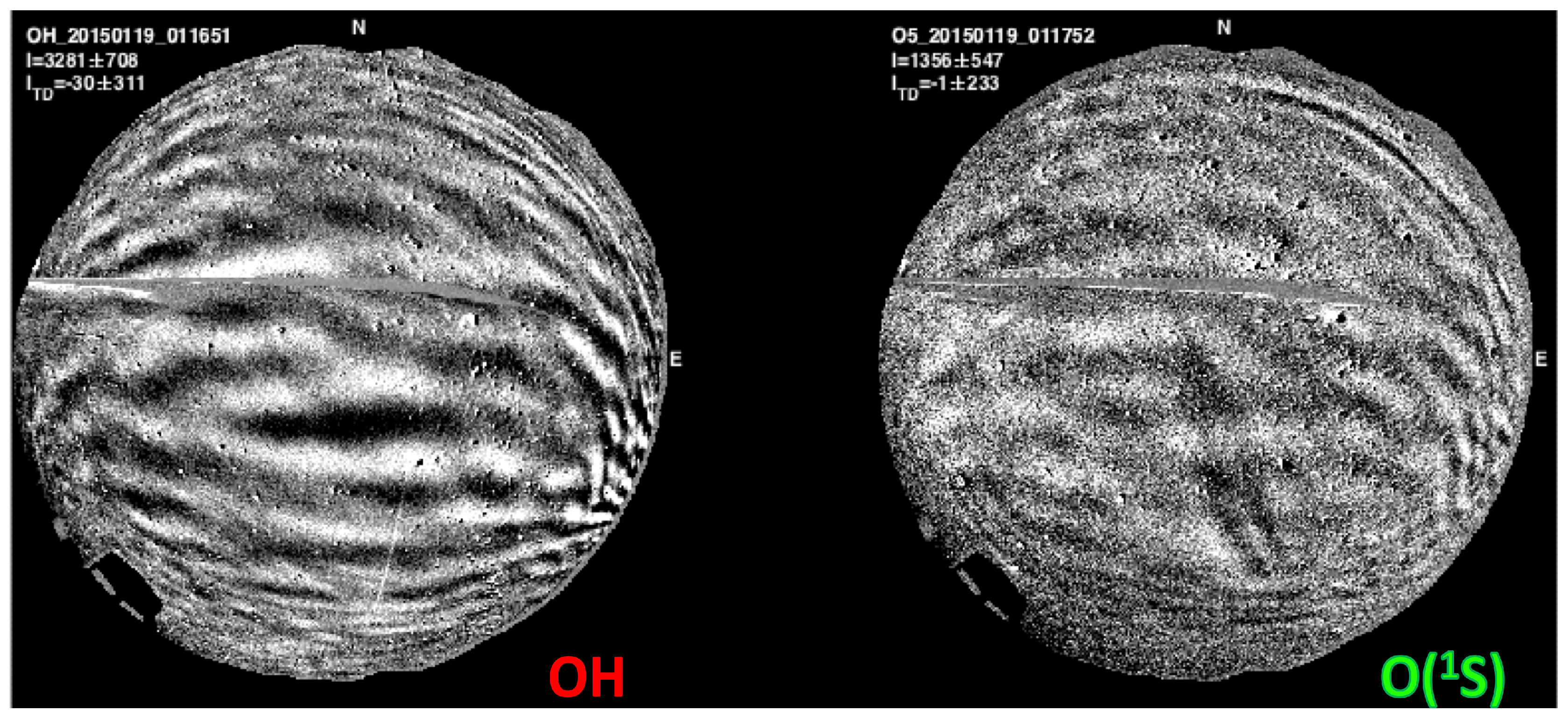
The ALO all-sky imager records nightglows of hydroxyl
Meinel bands and atomic oxygen line emissions (
Figure 1). The imager ASI-1 collects the nightglow emissions using the instrumental configuration presented in
Table 1. The ASI-1 images present a signal-to-noise ratio of better than 10 for the OH filter for image acquisition carried out during summer when the nightglow brightness is fainter.
The ALO lidar system transmits a nominal power of 1.5 W to obtain temperature, wind velocity, and Na density profiles typically at resolution of 1 min, 500 m between 80 and 105 km. The laser is a source of coherent light locked at the Na resonance frequency at the D2a line. This central frequency (f
) is shifted by ± 630 MHz to obtain the shifted frequencies f
and f
in a sequence to produce the optical excitation of the mesospheric sodium layer around the Na D2a line-width, enabling the production of an artificial beacon source. The temperature and line-of-sight wind are derived based on the ratios among the back-scattered signals at these three frequencies, as described in [
27]. The Na lidar is operated in zenith and off-zenith modes to measure the wind and temperature using the three-frequency technique (see [
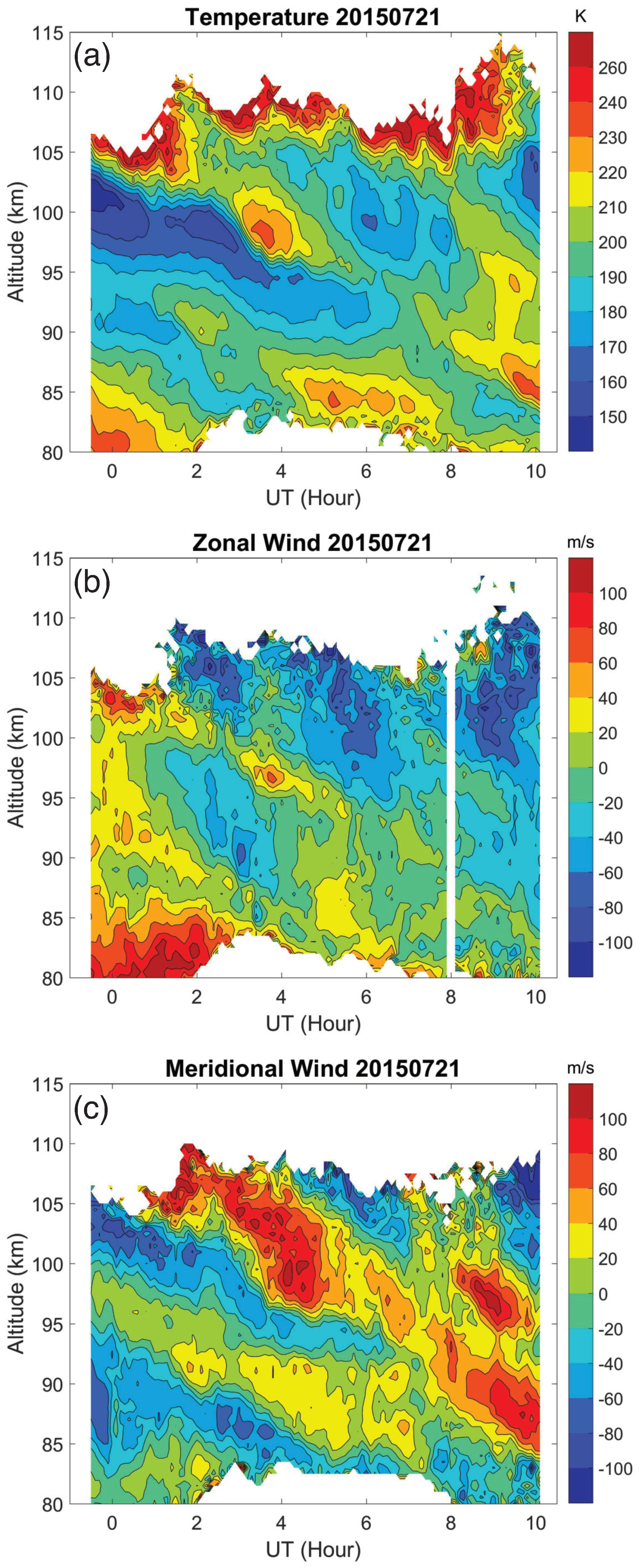
28]). The integration time for lidar scans varies between campaigns from 60 to 90 sec for each direction (zenith, south, east), which depends on the signal-to-noise ratio retrieved from the photon returns. As an example of the ALO lidar system capability, wind and temperature measurements versus time and altitude are shown in
Figure 2, although Na density and vertical wind velocity can still be estimated directly from ALO lidar scans.
Observations using the Na lidar and nightglow imagery system are carried out in low Moon periods throughout the year. All-sky images of the nightglow are taken simultaneously with the lidar, and individual gravity wave occurrence in both systems can be monitored during the observation time. The observations used in this study are summarized in
Table 2 and
Table 3. The imagery and lidar datasets were obtained at ALO during campaigns carried out during 2015, 2016, and 2017.
The modeled CF used here for comparison with our observational data was derived in [
21] using a linear, one-dimensional model to describe the temporal and spatial variability of the volume emission rate (VER) of a nightglow emission in response to AGW perturbations. The photochemistry involved in the processes leading to
production and the
Meinel band spectrum, as well as the intensity and weighted temperature due to upward propagating AGWs, is also described in [
21].
In order to maintain the solutions in the linear range, a number of assumptions were considered in the model including, for instance, that wave amplitudes are small (<1%) so that the AGW linear theory can be used to describe waves via the polarization and dispersion relationships. The wave perturbation of 1% amplitude is defined only in temperature at a reference altitude of z
km. Once the model considers only saturated waves, the wave amplitude does not change within the altitude range. The background atmosphere specified by the MSIS00 model is unchanged by the waves (e.g., [
29]). A windless atmosphere (no shear with altitude) where the waves are propagating vertically through the layers was also considered in the [
21] model. The simulations consisted of launching a gravity wave with
= 1% at z
, and then varying its vertical wavelength,
, and damping coefficient,
, in each iteration of the model. The resulting wave-perturbed nightglow VER and the intrinsic parameters of the simulated wave are then recorded for further analysis and fitting.
In addition, observed CF values were calculated for each individual gravity wave detected by our nightglow imager and lidar systems. Our methodology analyzes the perturbations of waves in nightglow images and also in lidar temperature in the vicinity of the nominal nightglow peak altitude. The observed CF, calculated using the observed perturbations, is defined for the nightglow intensity as
. Here,
and
, where primed quantities refer to the wave fluctuation and bar quantities to the unperturbed background.
is obtained from
and
nightglow image processing, and
from the lidar temperature data at the time of wave perturbation occurrence in the nightglow. The background temperature is estimated from the lidar measurements around the wave event occurrence time as the average temperature around ±2 wave periods. The observed CF is then compared to the CF model of [
21].
We have estimated the intrinsic wave parameters from the image dataset, such as the horizontal wavelength (
), wave orientation (
), wave phase (
), wave period (
), horizontal phase velocity (
c), and the relative wave amplitude (
), by performing the usual preprocessing routines (i.e., dewarping, star removal, coordinate transformation, detrending, and filtering as described in [
30]). At the preprocessing stage, each individual image is mapped onto a uniform 512 × 512 km
grid of pixels in geographical coordinates with a resolution of 1 km/pixel. The assumed altitudes for the
and
emissions were 88 and 95 km, respectively. The integration times used in this study were 60 s for the
and 90 s for the
. In particular, we used mean horizontal winds from the lidar to perform Doppler correction of wave periods.
The wave amplitude is obtained from the magnitude of the dominant peaks of the cross-spectrum of time-difference nightglow images. Only dominant wavenumber peaks with energy larger than 10% of the total spectrogram energy are considered as legitimate waves. This is determined from a series of three consecutive nightglow images materializing in the 2D-FFT amplitude cross-periodogram as prominent peaks. We only use a small area of the image to determine the wave amplitude as the fields of view of the imager and lidar are different. This small portion is a 172 × 172 km window centered at zenith. The lidar beam falls at the center of this window, at the image zenith. The wave amplitude in lidar temperature is estimated in time around the instant of occurrence of the wave observed in the nightglow images within a time window of ±2 wave periods around the occurrence time. For instance, if the wave period is 10 min, the time window is 40 min long. Hence, the wave amplitude is determined spatially, while the wave amplitude is determined temporally. This procedure is valid as the wave amplitude is independent of either the temporal or spatial coordinates.
In order to compute the temperature perturbations from lidar, we have removed the mean () of each temperature altitude to determine corresponding to the nominal altitude of the observed nightglows. Because we estimate the wave amplitude in temperature around the wave occurrence time, we assume the temperature perturbation is due to the same wave seen in the nightglow. Then, after selecting short wave periods ( h) from prominent gravity wave events detected in imaging data, we estimate the observed CF for the two nightglow emissions for these prominent waves.
The wave amplitude in T for each nightglow layer is obtained at representing the altitude of the layer. Again, and are the perturbed and unperturbed nightglow intensity from the images, respectively, while and represent the perturbed temperature the unperturbed temperature obtained at the nominal altitudes of the observed nightglows, respectively. The ratio between and perturbations is our experimental estimation of the magnitude of the CF. The range of the relative amplitudes in temperature and nightglow intensity has been chosen so it does not break the linearity of the solutions in the modeled CF. This way, the dispersion and polarization equations remain valid throughout the analysis.
We have also defined cutoff limits for filtering out waves presenting parameters not consistent with the modeled CF (
Table 4). This way, wave amplitudes obtained from the image processing are comparable to the model. Finally, we have taken the relative wave and temperature intensities to compare the observed cancellation factor against the modeled CF relationship in [
21]. The uncertainties shown in this paper have been derived by using Equation (11), the fitting coefficients presented in Table 1, and Equation (12) of [
26].
3. Results
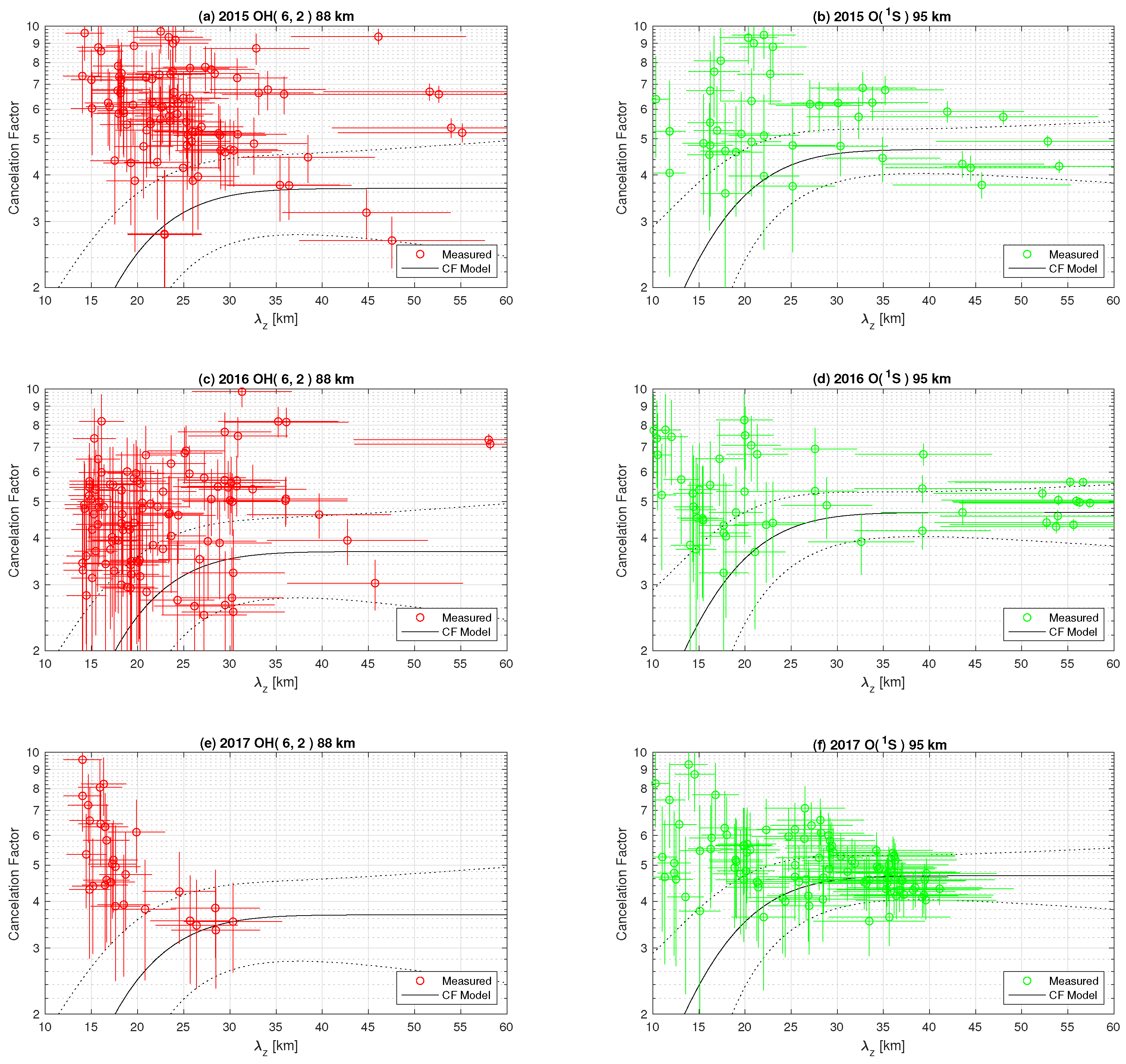
Prominent AGWs from the image processing were observed in 85 and 60 out of 100 nights of the initial sample for the
Meinel band emission and
emission line, respectively. After filtering the prominent wave events presented in
Table 2 using the criteria in
Table 4, 94 wave events remained on 11 nights in 2015, 113 waves through 19 nights in 2016, and 30 waves on 4 nights in 2017 campaigns associated with the
band emission. Following the same filtering procedure for the
emission line, 43 wave events remained for 9 nights in 2015, 50 waves for 9 nights in 2016, and 98 waves for 5 nights in 2017.
Table 5 summarizes these results for comparison purposes.
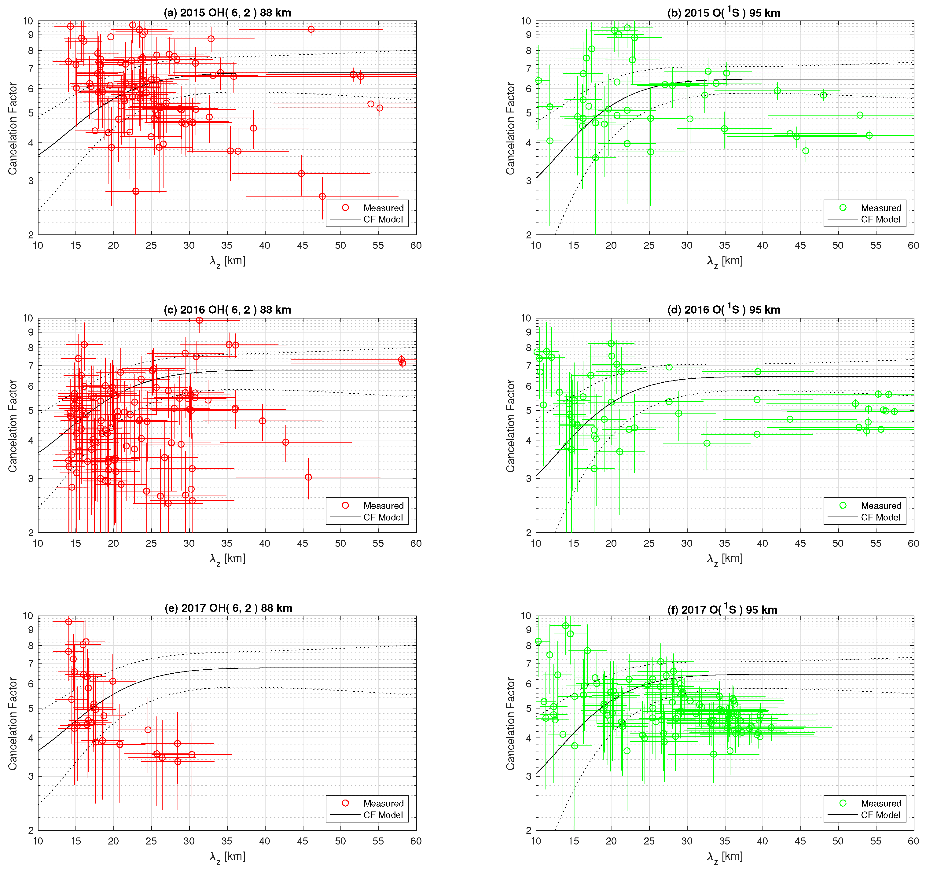
Figure 3 also shows the modeled CF error (dashed thin lines) that is dominated by the assigned error in
of ∼17%. This assigned error is the average of the error in the vertical wavelength of AGWs from nightglow observations. However, small errors in the modeled CF fitting coefficients also contribute to the overall error in the modeled CF. In addition, the observed CF error is calculated for each wave event using the methodology of [
26]. There are uncertainties in each wave parameter estimated from the nightglow observations that are transferred to the observed CF of each individual wave. These uncertainties also depend on the altitude of each emission. Observe that the errors in the individual observed CF values (
) and their associated vertical wavelength is shown in
Figure 3, which are estimated from Equations (8) and (12) of [
26]. It is expected that the relative uncertainty in CF (
) is a function of
and increases as
decreases.
The observed CF values are estimated for both
and
emission during 2015, 2016, and 2017 as shown in
Figure 3. The measurement of CF values for the
emission deviates from the theoretical CF relationship (black continuous lines) more than
, showing that the
has better agreement with the modeled CF in the range
20–60 km.
The uncertainties have been derived for
at the
and
emission altitudes. The average values are
16% and
17% for the
and
emissions, respectively. Reference [
26] found that
shows uncertainties of ∼10% and 8% for
and
emissions. The estimated uncertainties in observed CF are
10% for
emission and
7% for the green line
, respectively. The dotted thin lines in
Figure 3 represent the 95% confidence levels derived for the modeled CF. The uncertainties for both emissions range between 15 and 24%, and are higher for shorter
as expected.
Some observed CF data points fall within the modeled CF confidence levels (dashed thin lines) for the
emission (comparable to the full sample), which indicates those points are in agreement with the modeled CF relationship. To estimate how far the data points fall from the modeled CF curve, we have built histograms and kernel density estimators (KDEs) for the samples.
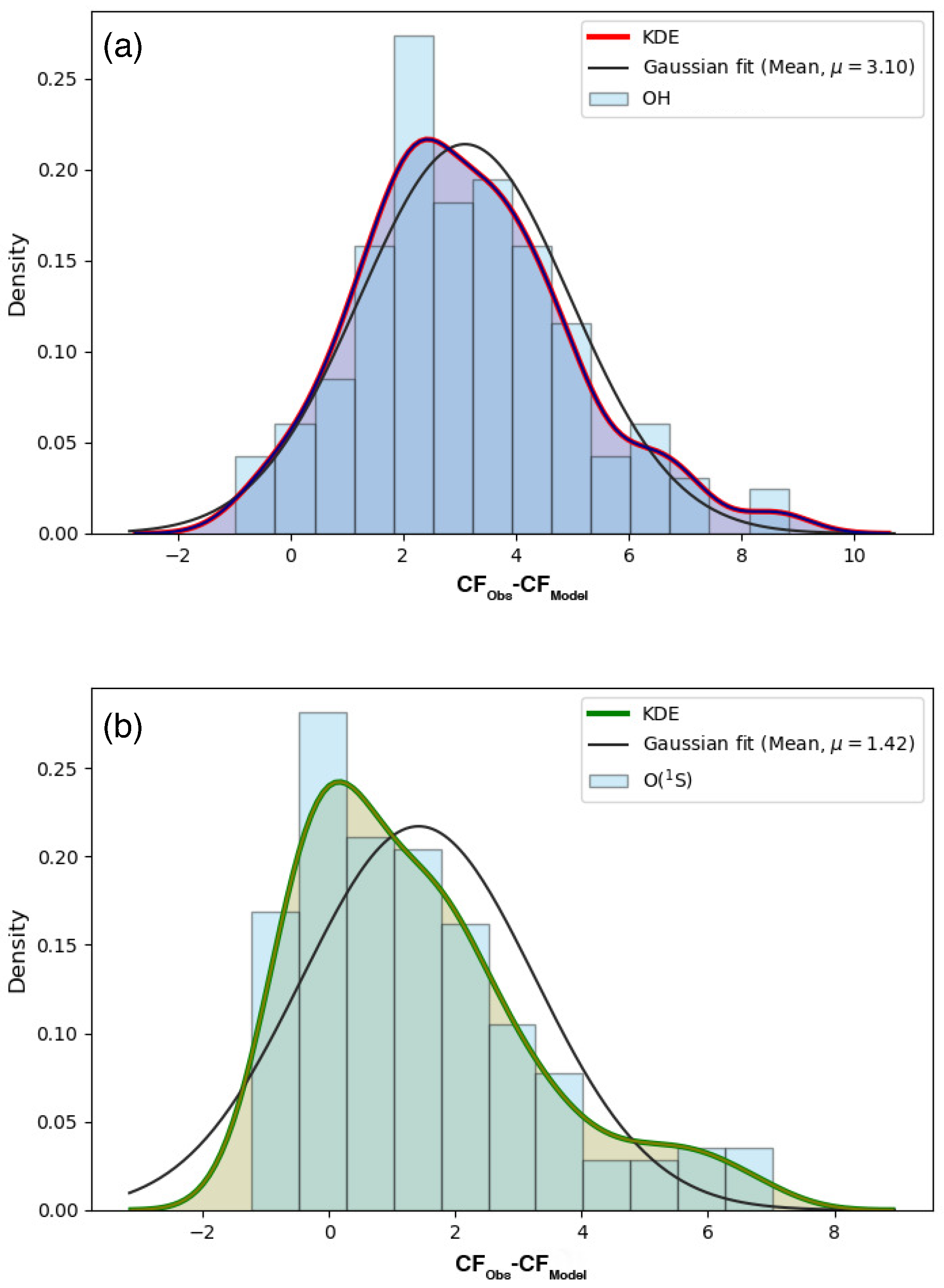
Figure 4 shows the residuals between the observed and modeled CF data points. The samples have been filtered out using a 3 times the standard deviation criteria to remove outliers.
The KDE curves (solid red line in
Figure 4) show the density plot as a smoother version of the histograms. The histograms are normalized by default so that they have the same y-scale as the density plots. In addition, we fitted a Gaussian function with bin width following the Freedman–Diaconis rule [
31], which changes the distribution drawn at each data point and the overall distribution. However, we have decided to use the Gaussian kernel density estimation to compute the mean values for both normal distributions.
The histograms in
Figure 4 have a well-defined central tendency in the normal distribution for both
and
emissions. The center of the CF
is closer to zero than CF
according to the mean value of the Gaussian curves. The peak of the distribution for both emissions is found to be skewed to the right, meaning that the model underestimates the observed values. The arithmetic mean values have been derived for the
and
emissions as
and
, respectively.
The main contribution of this work is to test the modeled CF relationship using the observed data. From that, we have verified that the theoretical model underestimates the observations. It is important to measure this discrepancy to make corrections to the theoretical relationship for both emissions. To do so, we have evaluated the discrepancy between observed and modeled CFs, and added them to the corresponding modeled CF for each layer to obtain corrected predictions. To estimate the discrepancy, we use the weighted mean and the standard deviation of the mean:
and
We use the weighted mean and standard deviation as they take into account the spread in the data (
Table 6). Data points presenting smaller uncertainties (
), that is, higher accuracy measurements, will have a larger influence on the weighted mean. This is better than using the arithmetical mean and standard deviation that just ignore the magnitude of the error of each measurement.
Note that the asymptotic value of the modeled CF is just the value of CF for very large
in
Figure 3. At this large scale range, CF tends to a stationary, unchanged value of 3.5 (5.1) for the
(
) emission. Thus, a measure of the discrepancy between modeled and observed CF takes into account the asymptotic value of the modeled CF of both layers. The calculated discrepancy is a simple way to provide an empirical correction to the modeled CF for the emissions, although further investigation into the CF model assumptions and parameters must be carried out. The corrected CF model curves are shown in
Figure 5.
The CF weighted mean and weighted errors computed for the emission lines in 2015, 2016, and 2017 are in good agreement with the modeled asymptotic value, CF4.5 for large values of . However, we did not find a good result for the CF= 3.5 asymptotic value, as the estimated weighted mean was much larger than in the model in the high wavelength range.
4. Discussion
We tested the modeled CF presented in [
21] for the Meinel
band emission and
emission line using observed data obtained from ALO. We reported perturbations in the nightglow intensity in response to the AGWs under cancellation effects modeled with an empirical method that considers a windless and isothermal atmosphere with upward propagating and saturated waves (the wave amplitude does not change with altitude).
Figure 3 shows the cancellation factors in both layers as functions of
. From the definition, we see that smaller CF corresponds to a stronger cancellation effect. Conversely, CF increases with increasing
up to an asymptotic value above the unit, showing that the wave amplitude is amplified by the layer response to the wave perturbation.
The intensity perturbations with small vertical scale (
km) have strong cancellation in the layer because of the finite thickness of the nightglow layers, which implies that these short
waves do not show significant amplitudes from ground observations ([
20]). Thus, the nightglow is not sensitive to these waves. Equation (11) presented in [
26] shows that the analytical function describing CF increases monotonically with
km for
band emission and
km for the
emission line; therefore, for
lower than these limits the cancellation effect gets stronger.
The centroid height and thickness (FWHM) of the unperturbed and standard deviations of the VER profiles derived for the
layer are larger than that the
layer (see Table 1 in [
21]), which results in a stronger cancellation effect in the
layer and therefore the CF for
emission is larger than that for
, indicating that the greenline nightglow is more sensitive to AGWs. For
larger than ∼20 km, the layer thickness becomes irrelevant because the layer thickness is a fraction of the vertical wavelength; the layer response is stronger and virtually the same for longer vertical wavelength waves.
The work of [
26] has presented a comprehensive discussion about the magnitude of the uncertainties in gravity wave parameters estimated from nightglow measurements, and how these uncertainties affect the estimation of key dynamic quantities in the mesosphere and lower thermosphere region. In this study, we derived the uncertainties in CFs and vertical wavelengths, which are subject to large uncertainties. However, these magnitudes are in agreement with conclusions reported in [
26].
A source of discrepancy between the modeled and observed CF values found in this study is that the CF model considers saturated waves only. In a real atmosphere, saturated waves co-exist with dissipative and freely propagating waves. That fact likely accounts for the majority of the discrepancy in our results because we have not separated waves by their kind in this study. As all observed wave cases go into our analysis for comparisons with the CF model, we cannot guarantee that the observed waves are saturated waves as in the CF model.
Another source of discrepancy in our results with the modeled CF for the
and
layers is relative to the distribution of atomic oxygen with height in the presence of vertically propagating waves, which could also influence the results here. The waves influence the temperature gradient that affects the rate of chemical reactions in the nightglow emissions ([
18]). The distribution of species involved in nightglow emissions varies considerably with latitude and time, constituting another source of discrepancy between model and measurements ([
32]) once the model considers only calm, low solar cycle atmospheric conditions.
In addition, based on a full-wave model with the relevant chemistry for the nightglow emissions that considers more physical processes such as propagating gravity waves in a non-isothermal mean state, and windy (background winds
as a function of height) and viscous atmospheres, the cancellation factors can vary considerably by a factor of two greater than isothermal and windless values for gravity waves of short horizontal wavelengths with phase velocities less than 100 m/s, and by a factor of one hundred for phase speeds less than 40 m/s as reported in [
32].
All in all, having tested the modeled CF relationship against observed data for two nightglow layers, we have found that the modeled CF underestimates the observations for both emissions. The cancellation effect is found to be larger in magnitude for
-band emission than for the
emission line. However, CF is still a valuable parameter for retrieving the magnitude of the relative temperature fluctuation from the nightglow, which is used to estimate the momentum flux magnitude transported by the waves ([
26]).
The impact of the empirical correction is most significant on momentum flux estimations for the
emission. For instance, [
33] estimated the vertical flux of horizontal momentum associated with an extensive and bright mesospheric gravity wave event that occurred over the El Leoncito Observatory, Argentina (31.8
S, 69.3
W), during the nights of 17 and 18 March 2016. The estimated average momentum flux of this spectacular wave was ∼232 m
/s
using the modeled CF of [
21], but according to our correction, this estimated value would be reduced by a factor of 3.4 as the momentum flux depends on CF
.


