Effects of Rear Angle on the Turbulent Wake Flow between Two in-Line Ahmed Bodies


Abstract
:
1. Introduction
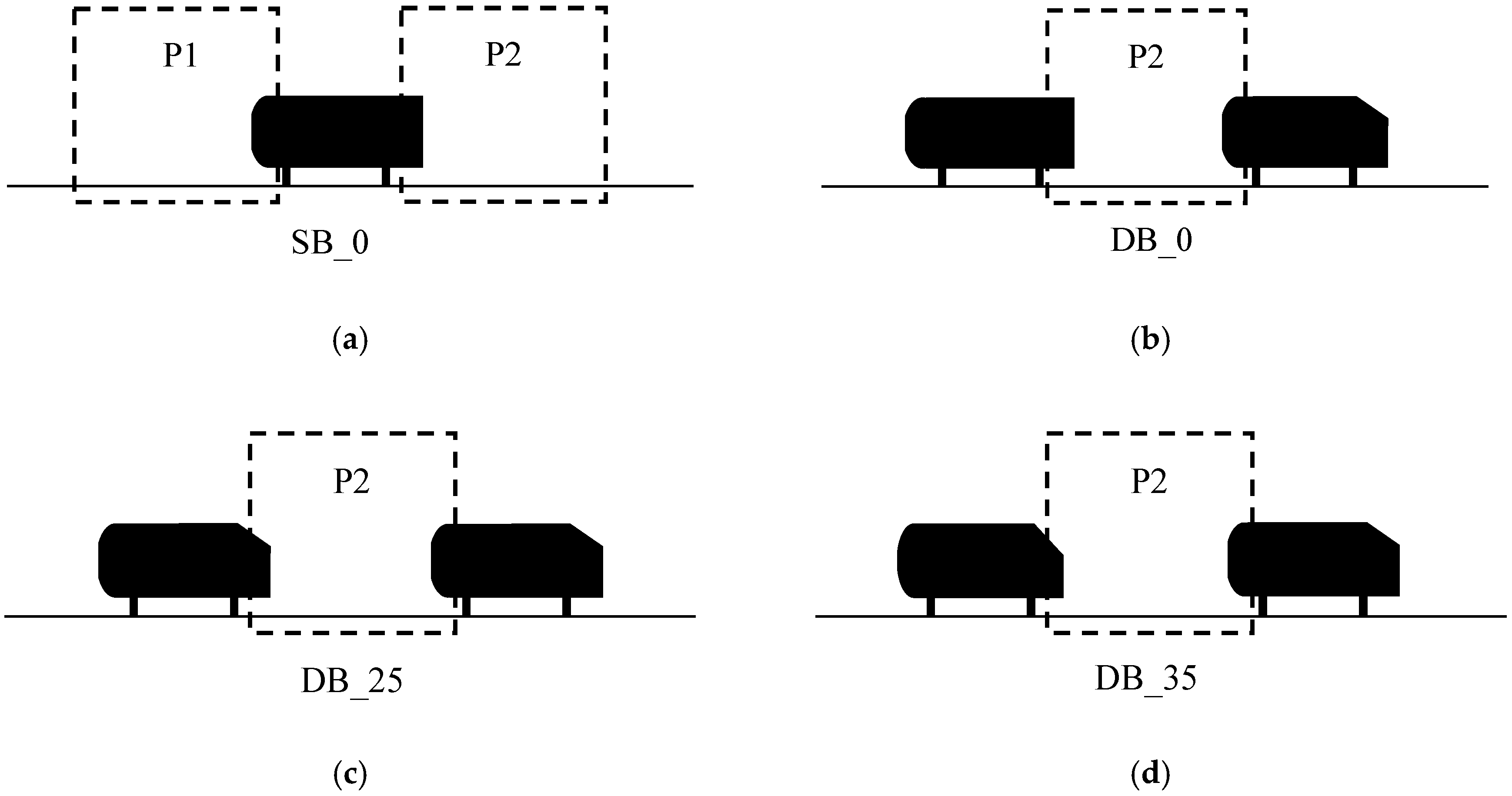
2. Experiments
3. Results
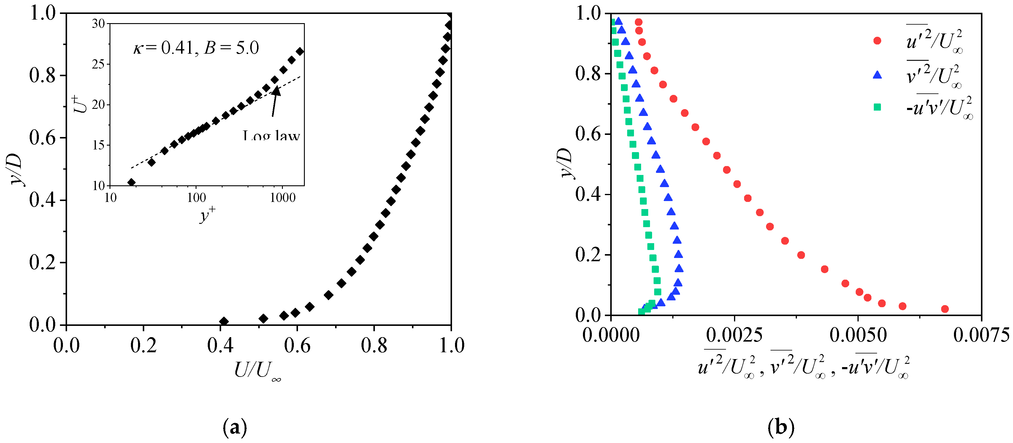
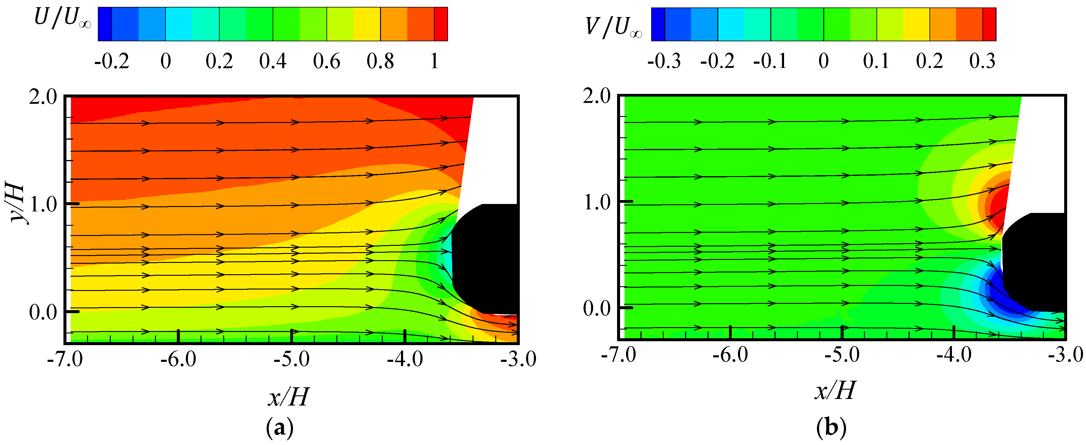
3.1. Approach Flow
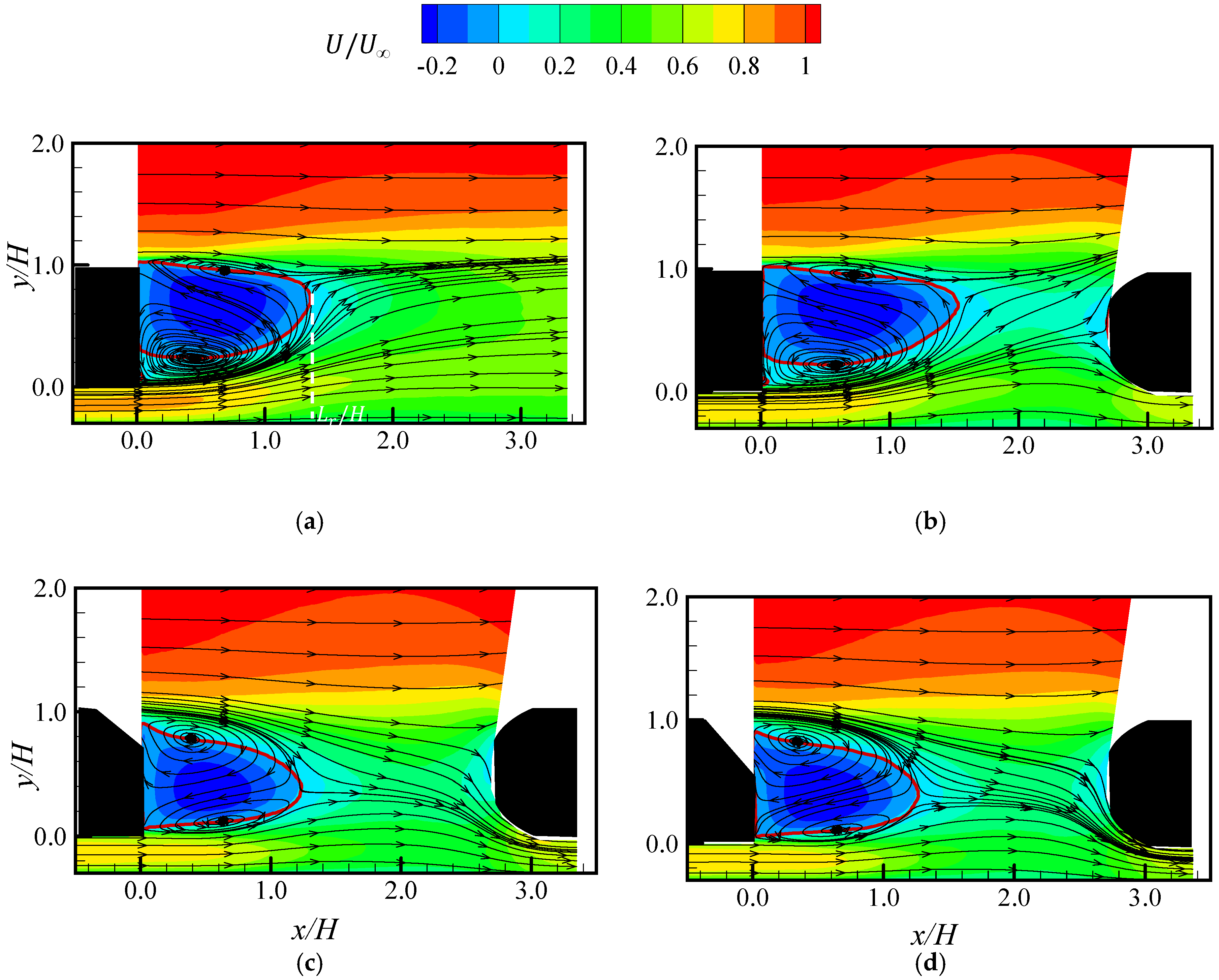
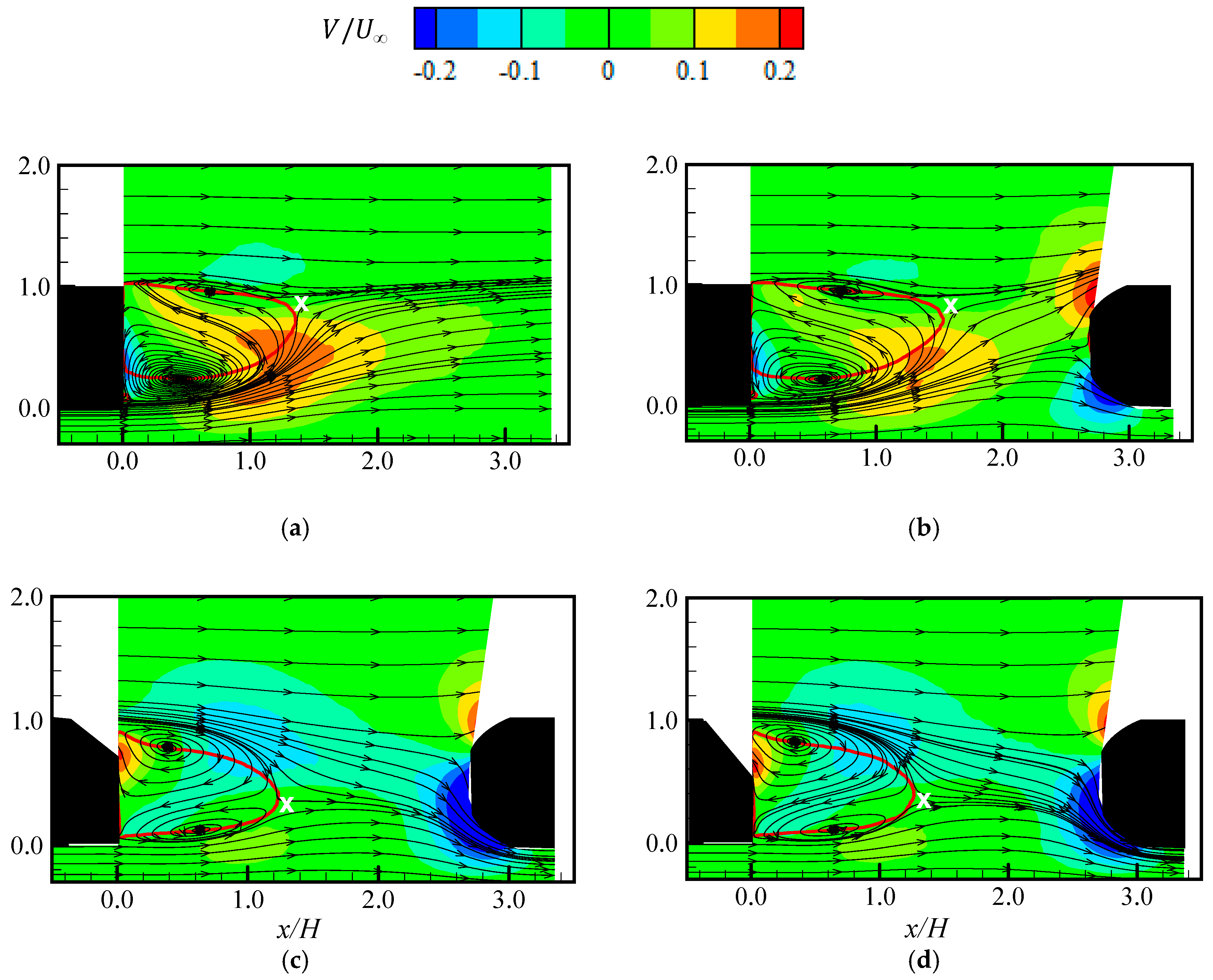
3.2. Streamwise and Wall-Normal Mean Velocities in the Wake Region
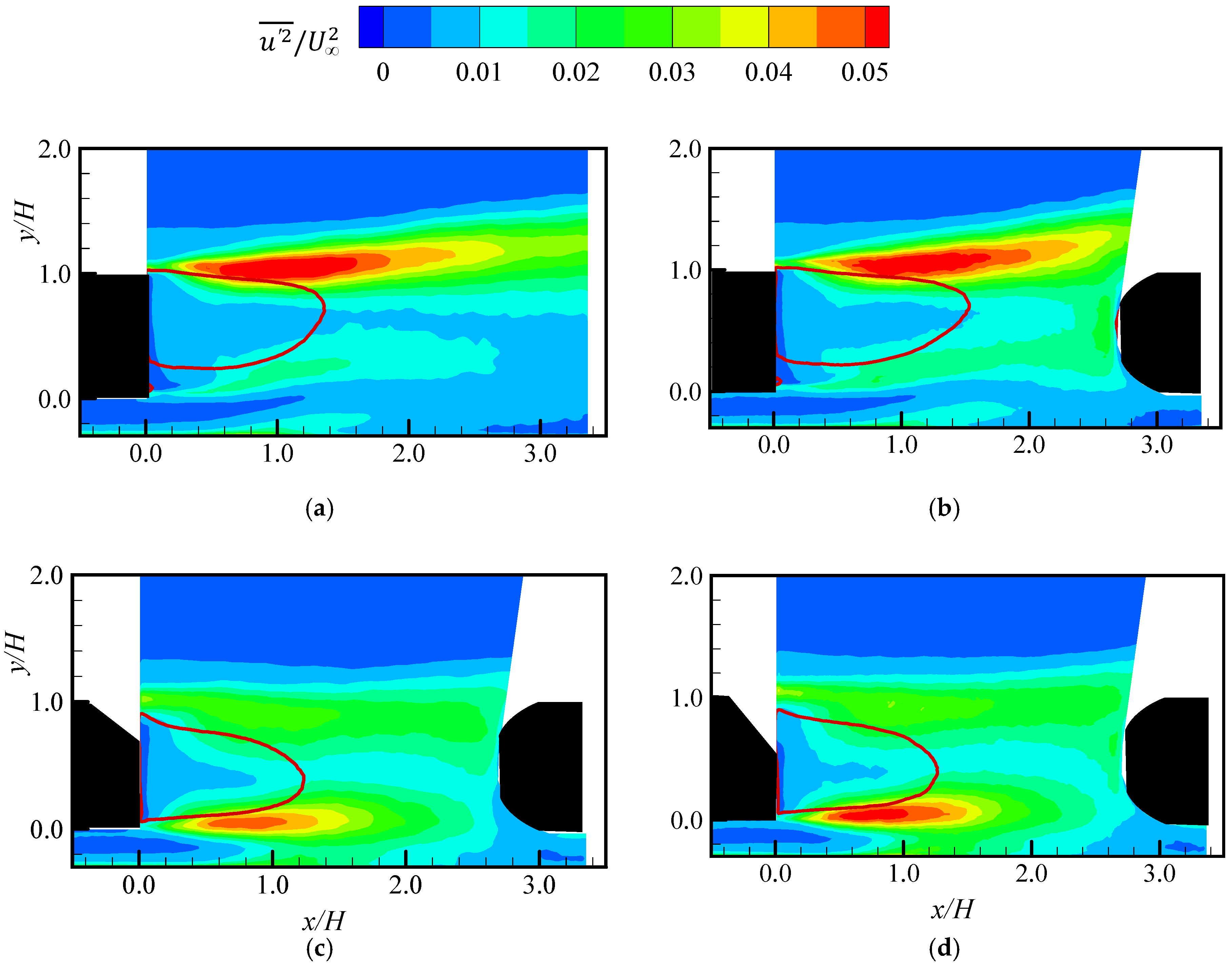
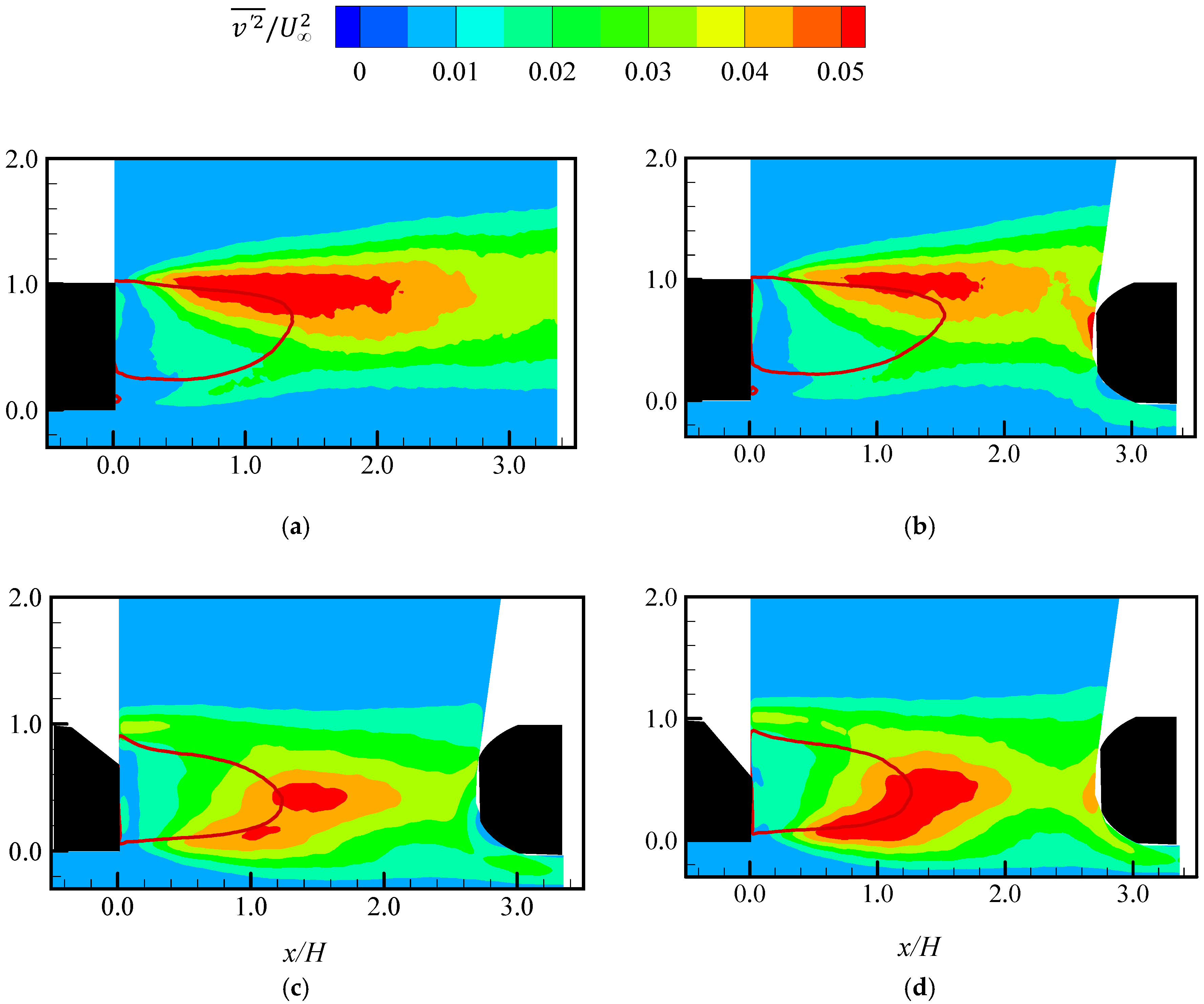
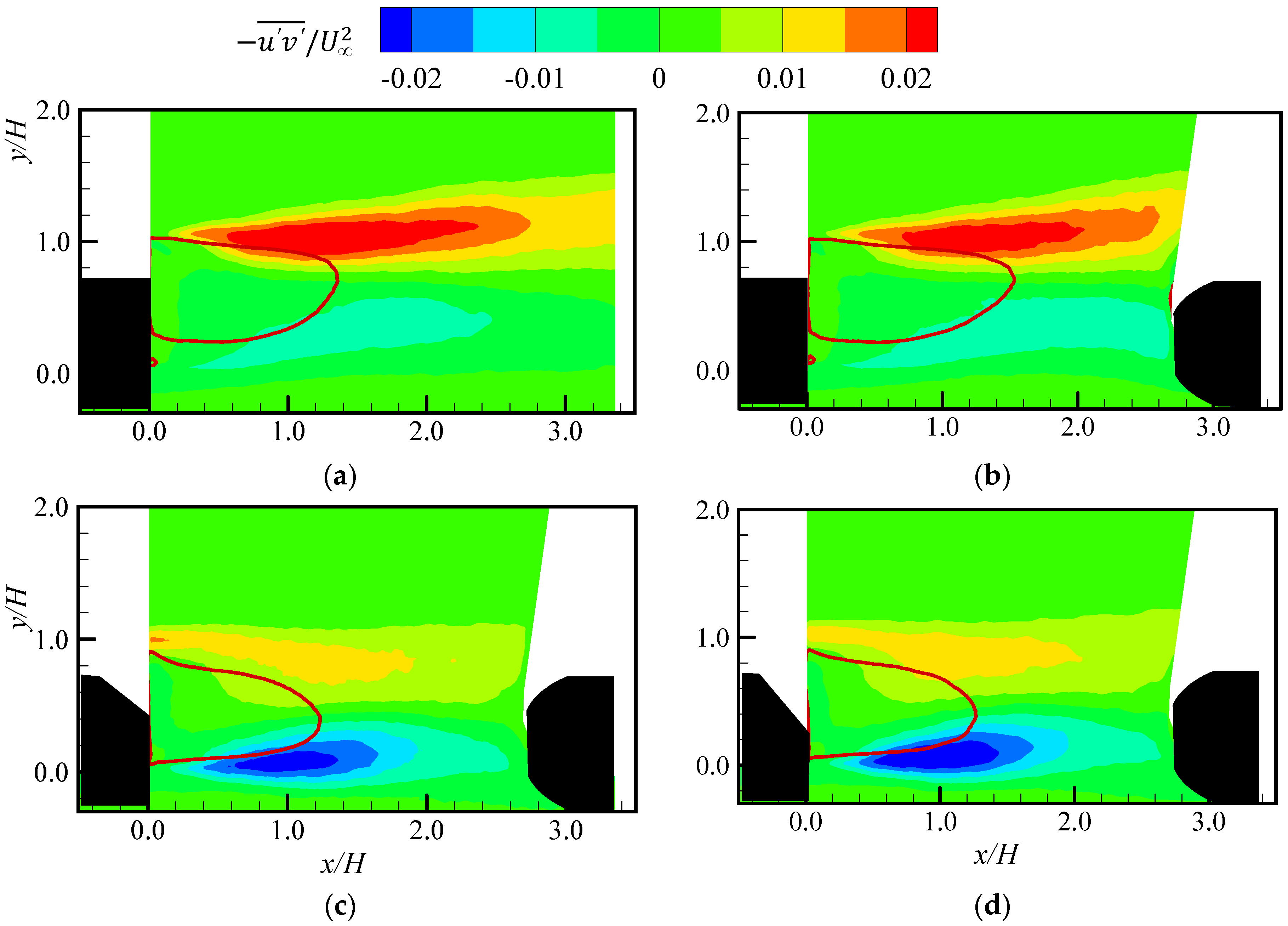
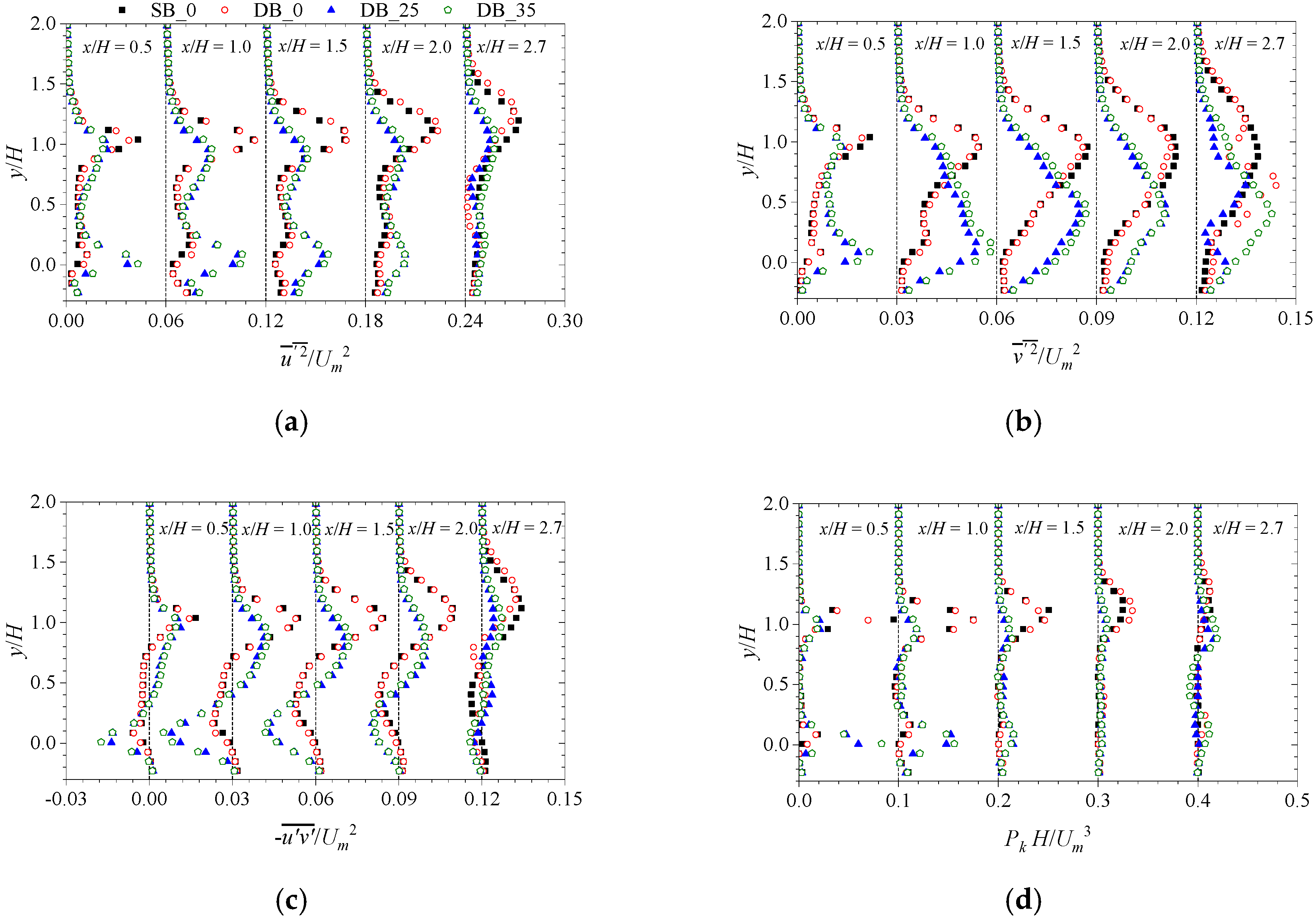
3.3. Reynolds Stresses and Turbulent Production in the Wake Region
3.4. Instantaneous Flow Structures
4. Conclusions
Author Contributions
Funding
Conflicts of Interest
References
- Knibbs, L.D.; de Dear, R.J. Exposure to ultrafine particles and PM2.5 in four Sydney transport modes. Atmos. Environ. 2010, 44, 3224–3227. [Google Scholar] [CrossRef] [Green Version]
- Xu, B.; Zhu, Y. Investigation on lowering commuters’ in-cabin exposure to ultrafine particles. Transp. Res. Part D Transp. Environ. 2013, 18, 122–130. [Google Scholar] [CrossRef]
- Pasquier, A.; André, M. Considering criteria related to spatial variabilities for the assessment of air pollution from traffic. Transp. Res. Procedia 2017, 25, 3354–3369. [Google Scholar] [CrossRef]
- Gan, W.Q.; Koehoorn, M.; Davies, H.W.; Demers, P.A.; Tamburic, L.; Brauer, M. Long-term exposure to traffic-related air pollution and the risk of coronary heart disease hospitalization and mortality. Environ. Health Perspect. 2011, 119, 501–507. [Google Scholar] [CrossRef] [PubMed]
- Brauer, M.; Hoek, G.; Van Vliet, P.; Meliefste, K.; Fischer, P.H.; Wijga, A.; Koopman, L.P.; Neijens, H.J.; Gerritsen, J.; Kerkhof, M.; et al. Air pollution from traffic and the development of respiratory infections and asthmatic and allergic symptoms in children. Am. J. Respir. Crit. Care Med. 2002, 166, 1092–1098. [Google Scholar] [CrossRef] [PubMed] [Green Version]
- Knibbs, L.D.; Cole-Hunter, T.; Morawska, L. A review of commuter exposure to ultrafine particles and its health effects. Atmos. Environ. 2011, 45, 2611–2622. [Google Scholar] [CrossRef] [Green Version]
- Rank, J.; Folke, J.; Homann Jespersen, P. Differences in cyclists and car drivers exposure to air pollution from traffic in the city of Copenhagen. Sci. Total Environ. 2001, 279, 131–136. [Google Scholar] [CrossRef]
- Gulliver, J.; Briggs, D.J. Personal exposure to particulate air pollution in transport microenvironments. Atmos. Environ. 2004, 38, 1–8. [Google Scholar] [CrossRef]
- Hudda, N.; Kostenidou, E.; Sioutas, C.; Delfino, R.J.; Fruin, S.A. Vehicle and driving characteristics that influence in-cabin particle number concentrations. Environ. Sci. Technol. 2011, 45, 8691–8697. [Google Scholar] [CrossRef] [PubMed]
- Murzyn, F.; Fokoua, G.; Rodriguez, R.; Shen, C.; Larrarte, F.; Mehel, A. Car Wake Flows and Ultrafine Particle Dispersion: From Experiments to Modelling. Atmosphere 2019, 11, 39. [Google Scholar] [CrossRef] [Green Version]
- Kaur, S.; Nieuwenhuijsen, M.J.; Colvile, R.N. Fine particulate matter and carbon monoxide exposure concentrations in urban street transport microenvironments. Atmos. Environ. 2007, 41, 4781–4810. [Google Scholar] [CrossRef]
- Abi-Esber, L.; El-Fadel, M. Indoor to outdoor air quality associations with self-pollution implications inside passenger car cabins. Atmos. Environ. 2013, 81, 450–463. [Google Scholar] [CrossRef]
- Ahmed, S.R.; Ramm, G.; Faltin, G. Some Salient Features of the Time -Averaged Ground Vehicle Wake. SAE Trans. 1984, 473–503. [Google Scholar]
- Minguez, M.; Pasquetti, R.; Serre, E. High-order large-eddy simulation of flow over the “Ahmed body” car model. Phys. Fluids 2008, 20. [Google Scholar] [CrossRef]
- Zhang, B.F.; Zhou, Y.; To, S. Unsteady flow structures around a high-drag Ahmed body. J. Fluid Mech. 2015, 777, 291–326. [Google Scholar] [CrossRef]
- Krajnović, S. Large Eddy Simulation Exploration of Passive Flow Control Around an Ahmed Body. J. Fluids Eng. 2014, 136, 121103. [Google Scholar] [CrossRef] [Green Version]
- Beaudoin, J.F.; Aider, J.L. Drag and lift reduction of a 3D bluff body using flaps. Exp. Fluids 2008, 44, 491–501. [Google Scholar] [CrossRef]
- Hucho, W.-H.; Sovran, G. Aerodynamics of Road Vehicles. Annu. Rev. Fluid Mech. 1993, 25, 485–537. [Google Scholar] [CrossRef]
- Rao, A.; Minelli, G.; Basara, B.; Krajnović, S. On the two flow states in the wake of a hatchback Ahmed body. J. Wind Eng. Ind. Aerodyn. 2018, 173, 262–278. [Google Scholar] [CrossRef]
- Tunay, T.; Sahin, B.; Ozbolat, V. Effects of rear slant angles on the flow characteristics of Ahmed body. Exp. Therm. Fluid Sci. 2014, 57, 165–176. [Google Scholar] [CrossRef]
- Wang, X.W.; Zhou, Y.; Pin, Y.F.; Chan, T.L. Turbulent near wake of an Ahmed vehicle model. Exp. Fluids 2013, 54, 1490. [Google Scholar] [CrossRef]
- Krajnović, S.; Davidson, L. Influence of floor motions in wind tunnels on the aerodynamics of road vehicles. J. Wind Eng. Ind. Aerodyn. 2005, 93, 677–696. [Google Scholar] [CrossRef]
- Watkins, S.; Vino, G. The effect of vehicle spacing on the aerodynamics of a representative car shape. J. Wind Eng. Ind. Aerodyn. 2008, 96, 1232–1239. [Google Scholar] [CrossRef]
- Mirzaei, M.; Krajnović, S. Large Eddy Simulations of Flow around Two Generic Vehicles in a Platoon. In Proceedings of the 5th International Conference on Jets, Wakes and Separated Flows (ICJWSF2015), Stockholm, Sweden, 15–18 June 2015; Springer: Cham, Switzerland, 2016; pp. 283–288. [Google Scholar]
- Mirzaei, M.; Pavlenko, A. Experimental and Numerical Study of Flow Structures between Two Ahmed Bodies with Various Inter-Body Distances; Springer: Basel, Switzerland, 2015; pp. 18–31. [Google Scholar]
- Mirzaei, M.; Krajnović, S. Numerical Study of Aerodynamic Interactions in a Homogeneous Multi-vehicle Formation. In Proceedings of the 5th International Conference on Jets, Wakes and Separated Flows (ICJWSF2015), Stockholm, Sweden, 15–18 June 2015; Springer: Cham, Switzerland, 2016; pp. 289–294. [Google Scholar]
- Gnatowska, R.; Sosnowski, M. The influence of distance between vehicles in platoon on aerodynamic parameters. EPJ Web Conf. 2018, 180, 2030. [Google Scholar] [CrossRef] [Green Version]
- Adrian, R.J.; Westerweel, J. Particle Image Velocimetry; Cambridge University Press: Cambridge, UK, 2011. [Google Scholar]
- Coleman, H.; Steele, W. Engineering application of experimental uncertainty analysis. AIAA J. 1995, 33, 1888–1895. [Google Scholar] [CrossRef]
- Pope, S.B. Turbulent Flows; Cambridge University Press: Cambridge, UK, 2000. [Google Scholar]
- Roussinova, V.; Biswas, N.; Balachandar, R. Revisiting turbulence in smooth uniform open channel flow. J. Hydraul. Res. 2008, 46, 36–48. [Google Scholar] [CrossRef]
- Afzal, B.; Faruque, M.A.; Balachandar, R. Effect of Reynolds number, near-wall perturbation and turbulence on smooth open-channel flows. J. Hydraul. Res. 2009, 47, 66–81. [Google Scholar] [CrossRef]
- Nezu, I.; Nakagawa, H. Turbulent Open-Channel Flows (IAHR Monograph); AA Balkema: Rotterdam, The Netherlands, 1993. [Google Scholar]
- Tachie, M.F.; Balachandar, R.; Bergstrom, D.J. Low Reynolds number effects in open-channel turbulent boundary layers. Exp. Fluids 2003, 34, 616–624. [Google Scholar] [CrossRef]
- Daly, S. Automotive Air Conditioning and Climate Control Systems; Elsevier: Amsterdam, The Netherlands, 2011. [Google Scholar]
- Perry, A.E.; Steiner, T.R. Large-scale vortex structures in turbulent wakes behind bluff bodies. Part 1. Vortex formation processes. J. Fluid Mech. 1987, 174, 233–270. [Google Scholar] [CrossRef]
- Pearson, D.S.; Goulart, P.J.; Ganapathisubramani, B. Turbulent separation upstream of a forward-facing step. J. Fluid Mech. 2013, 724, 284–304. [Google Scholar] [CrossRef] [Green Version]
- Plumejeau, B.; Delprat, S.; Keirsbulck, L.; Lippert, M.; Abassi, W. Ultra-local model-based control of the square-back Ahmed body wake flow. Phys. Fluids 2019, 31, 85103. [Google Scholar] [CrossRef]
- Grandemange, M.; Gohlke, M.; Cadot, O. Turbulent wake past a three-dimensional blunt body. Part 1. Global modes and bi-stability. J. Fluid Mech. 2013, 722, 51–84. [Google Scholar] [CrossRef] [Green Version]
- Zhou, J.; Adrian, R.J.; Balachandar, S.; Kendall, T.M. Mechanisms for generating coherent packets of hairpin vortices in channel flow. J. Fluid Mech. 1999, 387, 353–396. [Google Scholar] [CrossRef]
- Wu, Y.; Christensen, K.T. Population trends of spanwise vortices in wall turbulence. J. Fluid Mech. 2006, 568, 55. [Google Scholar] [CrossRef] [Green Version]


| Shape Factor | ||||||
|---|---|---|---|---|---|---|
| 0.31 | 38 000 | 4 300 | 1 700 | 2.4 | 1.31 | 0.003 |
| Parameters | SB_0 | DB_0 | DB_25 | DB_35 |
|---|---|---|---|---|
| 1.36 | 1.53 | 1.23 | 1.26 | |
| 0.87 | 0.98 | 0.74 | 0.81 | |
| Centroid | [0.63,0.63] | [0.73,0.62] | [0.59,0.43] | [0.61,0.44] |
| Upper bubble focus | [0.70,0.96] | [0.73,0.95] | [0.39,0.79] | [0.34,0.82] |
| Lower bubble focus | [0.46,0.24] | [0.58,0.22] | [0.64,0.12] | [0.64,0.11] |
© 2020 by the authors. Licensee MDPI, Basel, Switzerland. This article is an open access article distributed under the terms and conditions of the Creative Commons Attribution (CC BY) license (http://creativecommons.org/licenses/by/4.0/).
Share and Cite
Essel, E.; Das, S.; Balachandar, R. Effects of Rear Angle on the Turbulent Wake Flow between Two in-Line Ahmed Bodies. Atmosphere 2020, 11, 328. https://doi.org/10.3390/atmos11040328
Essel E, Das S, Balachandar R. Effects of Rear Angle on the Turbulent Wake Flow between Two in-Line Ahmed Bodies. Atmosphere. 2020; 11(4):328. https://doi.org/10.3390/atmos11040328
Chicago/Turabian StyleEssel, Ebenezer, Subhadip Das, and Ram Balachandar. 2020. "Effects of Rear Angle on the Turbulent Wake Flow between Two in-Line Ahmed Bodies" Atmosphere 11, no. 4: 328. https://doi.org/10.3390/atmos11040328