1. Introduction
Weather is a continuous, multidimensional, dynamic, and chaotic process, which makes weather forecasting a tremendous challenge. In several studies, numerical weather prediction (NWP) has been used to forecast the future atmospheric behavior based on the current state and physics principles of weather phenomena. For example, Sekula et al. [
1] tested the Aire Limitée Adaptation Dynamique Développement International High-Resolution Limited Area Model (ALADIN-HIRLAM) numerical weather prediction (NWP) system to predicted air temperatures in the Polish Western Carpathian Mountains. However, predicting spatial and temporal changes in temperature for complex terrains remains a challenge to NWP models. In another research, Frnda et al. [
2] proposed a model based on a neural network to improve the European Centre for Medium-Range Weather Forecasts (ECMWF) model output accuracy and pointed out the potential application of neural network for weather forecast development. Considering this, in the latest years, weather forecasting methods based on artificial neural networks (ANNs) have been intensively explored. Fahimi et al. [
3] considered and estimated Tehran maximum temperature in winter using five different neural network models and found that the model with three variables of the mean temperature, sunny hours, and the difference between the maximum and minimum temperature was the most accurate model with the least error and the most correlation coefficient. A survey on rainfall prediction using various neural network architectures have has been implemented by Nayak et al. [
4]. From the survey, the authors found that most researchers used a back propagation algorithm for rainfall prediction and obtained significant results. Furthermore, ANN models have been used for forecasting at differential scales, including long-term (yearly, monthly) [
5] and short-term (daily, hourly) [
6]. However, in most previous literature, the results acquired using ANN models were compared with those obtained using some linear methods, such as regression, autoregressive moving average (ARMA), and autoregressive integrated moving average (ARIMA) models [
7,
8,
9]. Agrawal [
10] implemented two different methods for modeling and predicting rainfall events, namely ARIMA and ANN. Finally, the research showed that the ANN model, which outperforms the ARIMA model, can be used as a suitable forecasting tool for predicting rainfall. In another research, Ustaoglu et al. [
11] applied three distinctive neural network methods, which were feed-forward back propagation (FFBP), radial basis function (RBF), and generalized regression neural network (GRNN) to forecast daily mean, maximum, and minimum temperature time series in Turkey and the results compared with a conventional multiple linear regression (MLR) method. In these cases, though the time series-based forecast was typically made under a linearity assumption, in practice, it was observed that the data being analyzed often had unknown nonlinear associations among them. However, ANNs provide a methodology to solve many types of nonlinear problems that are difficult to solve using traditional methods. Therefore, ANNs are suitable for weather forecasting applications because of their learning as well as generalization capabilities for nonlinear data processing [
12]. Nevertheless, because the temporal influence of past information is not considered by conventional ANNs for forecasting, recurrent neural networks (RNNs) are primarily used for time series analysis because of the feedback connection available in RNNs [
13]. Consequently, RNNs are well-suited for tasks that involve processing sequential data, including financial predictions, natural language processing, and weather forecasting [
14]. Long short-term memory (LSTM) is a state-of-the-art RNN, which makes it a strong tool for solving time series and pattern recognition [
15,
16]. This LSTM is often referred to as one of the most critical deep-learning techniques due to its long-term memory characteristic.
Deep learning is a work area of machine learning that is based on algorithms inspired by the structure (i.e., neural networks) and functionality of a human brain; these artificial structures are called artificial neural networks (ANNs). Deep learning enables machines to solve complicated tasks even if they highly varied, unstructured, and interconnected data. In recent years, because of their successful application in solving some of the most computationally challenging problems involving interactions between input and output factors, ANNs have attracted considerable interest. In particular, recent developments in deep learning have helped solve complicated computational problems in multiple areas of engineering [
17] as well as predict meteorological variables, such as rainfall [
18], wind speed [
19], and temperature [
3,
20]. Furthermore, neural networks, especially in deep-learning models, have numerous hyperparameters that researchers need to modify to obtain suitable results; these include a number of layers, neurons per layer, number of time lags, and the number of epochs. Choosing the best hyperparameters is essential and extremely time-consuming. After completely training the parameters of the model, hyperparameters are selected to optimize validation errors. The determination of these hyperparameters is subjective and strongly relied on the researchers’ experience. Thus, despite the advantages of neural network and deep-learning machine, issues related to the appropriate model specification exist in practice [
21,
22].
The “meta-learning” technique was introduced by some previous literature. Lemke and Gabrys [
23] presented four different meta-learning approaches, namely neural network, decision tree, support vector machine, and zoomed ranking to acquire knowledge for time series forecasting model selection. Additionally, a feed-forward neural network model call group of adaptive models evolution (GAME) was proposed by Kordik et al. [
24] to apply a combination of several optimization methods to train the neurons in the network. In the current study, meta-learning can be viewed as a process of “learning to learn” and is related to the techniques for hyperparameter optimization. In particular, the genetic algorithm (GA) was integrated with neural network models to obtain an appropriate one-day-ahead and multi-day-ahead forecasting model of the maximum temperature time series. Shortly, GA was used to determine the ideal hyperparameters of the neural network models to achieve the best solution and optimize forecast efficacy for maximum temperature [
25]. The capacity of GA in training ANNs and the deep-learning LSTM model for short-term forecasting was noted in some previous literature. Chung and Shin [
26] proposed a hybrid approach of integrating genetic algorithm (GA) and ANN for stock market prediction. Similarly, Kolhe et al. [
27] also introduced the combination of GA and ANN to forecast short-term wind energy, and this method obtained more efficient and accurate results compared to the ANN model. As far as we know, no research has been performed on applying the meta-learning technique to the deep-learning model (LSTM) especially in a meteorological forecasting has been studied. The objective of the current study was to investigate the potential of different neural networks, via ANN, RNN, and LSTM, for time series-based analysis and examine their applicability for weather forecasting.
The remainder of this paper is organized as follows: In
Section 2, the description of the employed neural network (NN) models is introduced.
Section 3 is dedicated to an explanation of the data used for experiments and the application methodology is described in
Section 4.
Section 5 provides the prediction results of daily maximum temperature at the Cheongju station in South Korea. Finally, we offer our conclusions in
Section 6.
4. Application Methodology
Our research relied closely on open source libraries under the Python environment [
33]. Python is an interpreted, high-level programming language that can be used for a wide variety of applications, including research purposes. Our models were implemented using the Keras [
34] toolkit, written in Python and TensorFlow [
35], an open-source software library provided by Google. Additionally, other important packages such as NumPy [
36], Pandas [
37], and Matplotlib [
38] were also used for processing, manipulating, and visualizing data.
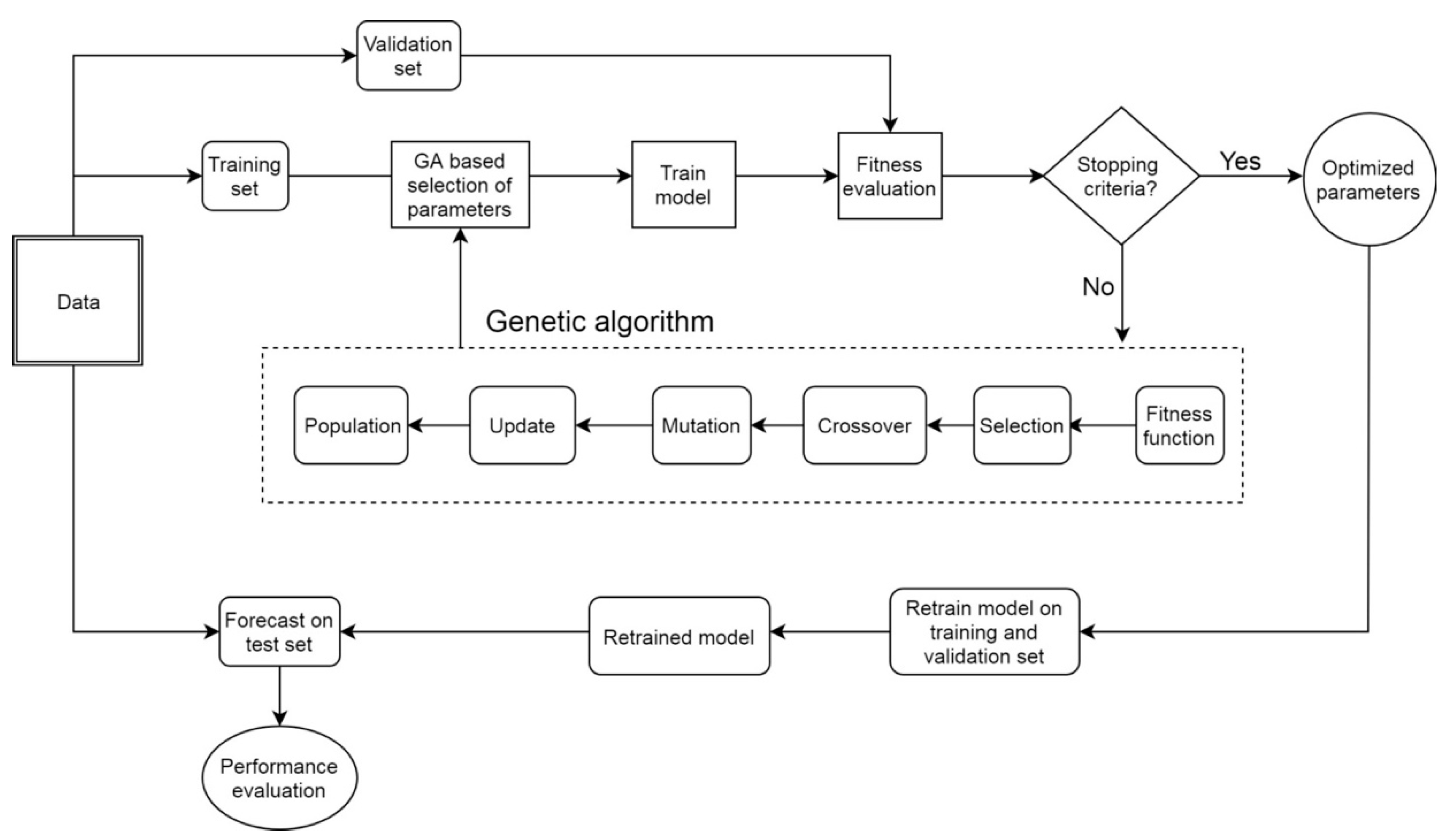
In this section, we discussed the experimental methodology for the three state-of-the-art deep learning model, LSTM as well as ANN and RNN in detail. The dataset was divided into three sets as training, validation, and test sets. The training set was used to train the model, the validation set was used to evaluate the network’s generalization (i.e., overfitting), and the test set was used for network performance assessment. In the current study, 80% of the data (1976–2007) was selected as the training set, while the remaining 20% (2008–2015) was used as the test set. Furthermore, within the training set, a validation of 20% training set (2001–2007) was set aside to validate the performance of the model and preventing overfitting. In particular, the validation set was used for the hyperparameter optimization procedure, which is described later. We used the training set to fit models and made predictions corresponding to the validation set, then measured the root mean square error (RMSE) of those predicted values. Lastly, we determined the value of hyperparameters of the model by selecting the smallest RMSE on the validation set (optimum model) using the genetic algorithm (GA) as explained as follows:
We fit a training set with three different neural network models, namely ANN, RNN, and LSTM. Genetic parameters, such as crossover rate, mutation rate, and population size, can influence the outcome to obtain the optimal solution to the issue. In this research, we used in the experiment a population size of 10, 0.4 for crossover rate, and 0.1 for mutation rate [
17]. A number of neurons in each hidden layer from 1 to 20, the number of epochs from 20 to 300, and the number of hidden layers from 1 to 3 will be evaluated. The tanh function is used as an activation function of the input and hidden neurons, while a linear function is designated as an activation function of output neurons in models. Initial weights of the network are set as random values, and a gradient-based “Adam” optimizer was used to adjust the network weights. GA solution would be decoded to get an integer number of epochs and a number of hidden neurons, which would then be used to train models. After that, RMSE on the validation set, which acts as a fitness function in this study, will be calculated. The solution with the highest fitness score was selected as the best solution. We implemented GA using distributed evolutionary algorithms in Python (DEAP) library [
39].
Figure 3 illustrated the flowchart of the hybrid model proposed in our work.
For each model, the dataset was trained with various cases of hidden layers, including one, two, and three hidden layers separately. The tanh function is used as an activation function of the input and hidden neurons while a linear function is designated as an activation function of output neurons in models. Initial weights of the network are set as random values, and a gradient-based “Adam” optimizer was used to adjust the network weights. GA solution would be decoded to get an integer number of epochs and number of hidden neurons, which would then be used to train models. After that, RMSE on the validation set, which acts as a fitness function in this study, will be calculated. The solution with the highest fitness score was selected as the best solution.
Genetic parameters, such as crossover rate, mutation rate, and population size, can influence the outcome to obtain the optimal solution to the issue. In this research, we used in the experiment a population size of 10, 0.4 for the crossover rate, and 0.1 for the mutation rate [
15]. A number of neurons in each hidden layer from 1 to 20, the number of epochs from 20 to 300, and the number of hidden layers from 1 to 3 will be evaluated. The number of generations is allocated as 10 as a terminated condition [
24]. We implemented GA using distributed evolutionary algorithms in Python (DEAP) library [
28].
We fitted the model with optimal hyperparameters for both training and validation sets, and then used the test set for forecasting. Experiments were performed one- and multi-step-ahead prediction. At first, we forecasted one-day-ahead maximum temperature. Using the lag time technique, we split the time series into input and output. For modeling simplicity, in this study, past seven daily data values
were employed to predict the daily maximum temperature for the next time (
). To estimate the prediction accuracy and evaluate the performance of the forecast, three performance criteria, namely root mean square error (RMSE) (see Equation (12)), squared coefficient of correlation (
) (see Equation (13)), and mean absolute error (MAE) (see Equation (14)) were used; these can be calculated as follows:
where,
is the current true value,
is its predicted value, and
n is the total number of testing data.
RMSE and MAE are commonly used to measure the difference between the predicted and observed values, while R2 indicates the fitness of the model to predict the maximum temperature. Furthermore, RMSE can be used to evaluate the closeness of these predictions to observations, while MAE can better represent prediction error. The ideal values of MAE and RMSE are definitely zero and R2 is certainly one, so the performance of a model obtains higher when the values of MAE and RMSE are close to zero and R2 is close to one. Each model (ANN, RNN, and LSTM) was fitted to the data for predicting one-day-ahead maximum temperature for the following three cases independently; using one-hidden-layer, two-hidden-layers, and three-hidden-layers.
Secondly, a multi-step ahead forecasting task was performed for predicting the next
h values
of a historical time series
composed of
m observations (lags). In order to obtain a multi-step-ahead prediction, we used the iteration technique [
40], i.e., a prediction
was used as input to obtain the prediction
for the next time step. Finally, we had a sequence of predictions
after
h iteration steps. In the beginning, seven values were used as inputs for the first prediction. Moreover, it has been calculated that the more maximum temperature values were appended as inputs for the first prediction, the longer the predictions were produced more accurately. Thus, seven to thirty-six past temperature data (lags) were used as inputs for the first output. This work has been done for four seasons using ANN, RNN, and LSTM. In the current study, the best-defined architecture (number of epochs, number of hidden neurons, and number of hidden layers) for each of the distinct models (ANN, RNN, and LSTM) was selected to forecast 2-15-day-ahead maximum temperature in order to compare the efficiency of the different models for prediction with long lead times. The performance was measured by RMSE. Furthermore, as described above, we employed the different number of lags (7–36) for ANN, RNN, and LSTM models in each season to investigate the best number of lags based on the RMSE of 15-day-ahead prediction. The results from some trial runs revealed that increasing the number of lags beyond this level did not reduce the error for any of models considered, the experiment was stopped at 36 lags. The scatter plot of maximum temperature for four seasons was shown in
Figure 4, which depicted the linear relationship between distinct lead times. As shown in
Figure 4, most of the points in winter, spring, summer, and autumn followed a linear relationship. However, owing to some points with large variations from the linear relationship, it might be difficult for the models to learn the underlying pattern. Additionally, it can be observed that the association of the variable in summer in high values is higher than in low values for one-day-ahead, which can suspect that models might capture the pattern of high values better than low values. As the lead time increased, the patterns of data in winter and summer were considerably dispersed. Furthermore, the wide range of higher values in winter got wider at long lead times (
k). In contrast, the lower values in spring, summer, and autumn expanded largely for longer range forecast.
6. Conclusions
In the current study, we applied the time series forecasting models of meteorological variables including the deep learning model (i.e., LSTM) assisted with the meta-learning for hyperparameter optimization. In particular, we forecasted the daily maximum temperature at the Cheongju station, South Korea up to 15 days in advance using the neural network models, ANN, and RNN as well as the deep-learning-based LSTM model. We integrated these models with GA to include the temporal properties of maximum temperature and utilized the customized architecture for the models.
GA was employed to obtain the optimal or near-optimal values of the number of epochs and the number of hidden units in neural network models through a meta-learning algorithm. Our results indicated that the LSTM model performed fairly well for long time scales in summer and spring than the other tested models in the current study. This can be attributed to the ability of LSTM models to maintain long-term memories, enabling them to process long sequences. In summary, the overall results demonstrated that the LSTM-GA approach efficiently maximum temperature in a season taking into consideration its temporal patterns.
This study shows that selecting the appropriate neural network architecture was important because it affected the temporal pattern and trend forecasting. To the best of our knowledge, in much of the existing literature, wherein neural networks were used to solve in time series problems, trial-and-error based methods rather than systematic approaches were used to obtain optimal hyperparameter values. However, we solved this issue by adopting GA, named as meta-learning. Our empirical results indicate the effectiveness of our proposed approach. Furthermore, the prediction that we made for the maximum temperature could be extended to other variables, including precipitation and wind speed. Thus, the method adopted in this study could be useful in determining the weather trend over a long-time period in a specific area.

 ,
, 


