Damage Analysis of Three Long-Track Tornadoes Using High-Resolution Satellite Imagery

Abstract

Remote sensing of tornado damage can provide valuable observations for post-event surveys and reconstructions. The tornadoes of 3 March 2019 in the southeastern United States are an ideal opportunity to relate high-resolution satellite imagery of damage with estimated wind speeds from post-event surveys, as well as with the Rankine vortex tornado wind field model. Of the spectral metrics tested, the strongest correlations with survey-estimated wind speeds are found using a Normalized Difference Vegetation Index (NDVI, used as a proxy for vegetation health) difference image and a principal components analysis emphasizing differences in red and blue band reflectance. NDVI-differenced values across the width of the EF-4 Beauregard-Smiths Station, Alabama, tornado path resemble the pattern of maximum ground-relative wind speeds across the width of the Rankine vortex model. Maximum damage sampled using these techniques occurred within 130 m of the tornado vortex center. The findings presented herein establish the utility of widely accessible Sentinel imagery, which is shown to have sufficient spatial resolution to make inferences about the intensity and dynamics of violent tornadoes occurring in vegetated areas.

1. Introduction

Short-term meteorological events such as severe thunderstorms and tornadoes can leave lasting effects on the natural landscape. Wind, hail, and tornado damage to forests and agricultural regions can be severe enough to identify with both ground level observations [1,2,3,4,5] and satellite imagery [6,7]. Aerial imagery of tornado damage has been used since the mid-20th century and allows for a “birds-eye” view to identify patterns that may not be discernible at ground-level, or would otherwise be unidentified [8,9]. This approach can be particularly useful in rural or remote regions that are difficult to survey after the event because they are inaccessible at ground level [10,11,12,13]. Additionally, tornado intensity is difficult to infer in areas where damage indicators are lacking [10]. Recent advances in moderate- and high-resolution multispectral imagery have allowed for further study of vegetation damage by tornadoes [12], as well as tornado characteristics that may not be apparent at the ground level, including the extent of tornado path and effects of local topography [14,15,16]. These techniques are most effective when using imagery with a high spatial resolution in regions of strong damage and homogenous land cover [17,18]. Normalized Difference Vegetation Index (NDVI, used as a proxy for vegetation health) differences and principal components techniques can be used to discern damage as weak as (E)F-1 [14,19,20] on the Enhanced Fujita (EF) scale, with more pronounced decreases in NDVI corresponding to greater damage in stronger tornadoes [14,21]. NDVI difference calculated from an image obtained before the tornado event and an image obtained after the event, as is performed in this study, is an effective tool in damage identification [14]. However, debris removal and other non-meteorological processes occurring in the weeks after the event can also affect NDVI in ways that are not a direct function of damage severity [14]. Additionally, the seasonal fluctuation of NDVI affects its utility in monitoring longer-term recovery [18]. Photosynthetic activity may be stunted or stopped completely in vegetation damaged by the tornado, and forest damage has been observed to persist for months, relative to nearby undamaged areas [18]. These factors must be taken into account when selecting imagery for differencing-based methods.

Tornadoes can be modeled by a Rankine vortex. In this model, solid body rotation occurs within the vortex, with rotational velocity increasing linearly from the center of the vortex to the radius of maximum winds, and then decreasing hyperbolically outside this radius. Early tornado researchers such as Johannes Letzmann [22] noted that the translational velocity of the tornado through space is added to the cyclonic rotational velocity of the vortex, and the strongest wind speeds are found at the radius of maximum winds on the right flank of a cyclonically rotating tornado, confirmed by later observational studies [9]. Rankine and related models of tornado vortices are further discussed in Wood and White (2011; 2013), and Kim and Matsui (2017) [23,24,25]. Applications of Rankine vortex models to identify tree fall patterns in forests have been performed either through modelling or tree fall digitization with aerial imagery [26,27,28]. These studies found that tree falls were more common on a tornado’s right flank than on its left flank, with the difference in vegetation damage between flanks mainly dependent on $G_{max}$, the ratio of the translational velocity of the tornado to its rotational velocity. Karstens et al. (2013) [28] and Cannon et al. (2016) [15] found evidence of other microscale phenomena such as Venturi enhancement of damage in valleys and increased damage on downslopes during vortex stretching. These studies confirm that tornado vortex dynamics can be discerned with vegetation damage in remote areas lacking damage indicators from the built environment, which complicates tornado intensity estimation in these regions [10]. While methods to estimate EF-scale using tree damage in dense forests have recently been explored [11], climatological research has found a bias in EF-ratings towards developed landcovers [29], suggesting that the intensity of tornadoes in rural areas may be systematically underestimated.

Recent advances in remote sensing technology have allowed for high-resolution imagery to be obtained by satellite-borne sensors such as Sentinel-2 MultiSpectral Instrument (MSI). The purpose of this research is to correlate products derived from Sentinel-2 imagery with wind speeds estimated in the post-event surveys [30,31], as well as to compare remotely sensed damage signatures across the width of the tornado path with wind speeds in the Rankine vortex model. This study is one of the first to conduct tornado damage assessment using Sentinel-2 imagery, which is perhaps the finest-scale imagery that is currently both regularly collected and freely available, making it a rich and accessible data source. The Rankine vortex model has been applied to case studies of violent tornado damage using aerial imagery [28] and building surveys [32], but this study is among the first to do so using satellite-derived NDVI. NDVI is an easily calculable, well-established metric that, provided with adequately clear imagery, can be applied to future case studies without the time or resources needed to perform ground surveys or acquire aerial imagery. It is also among the first to examine the Beauregard–Smiths Station tornado, one of the most violent of 2019, in detail. This tornado occurred in a vegetated region during the early spring green-up period, which represents the ideal conditions for damage analysis using a vegetation index such as NDVI. Specific research objectives (ROs) for this study are:

RO #1: To determine the correlation between estimated wind speed at damage indicators identified in post-event surveys and NDVI-difference at those locations;

RO #2: To identify a similar or stronger correlation using a principal components analysis involving imagery obtained both before and after the tornadoes;

RO #3: To identify the pattern of NDVI-differenced and principal component values across the lateral width of the tornado tracks, perpendicular to storm motion;

RO #4: To compare the pattern identified for RO #3 to the wind field across the lateral width of a tornado as modeled by a Rankine Vortex.

2. Methods

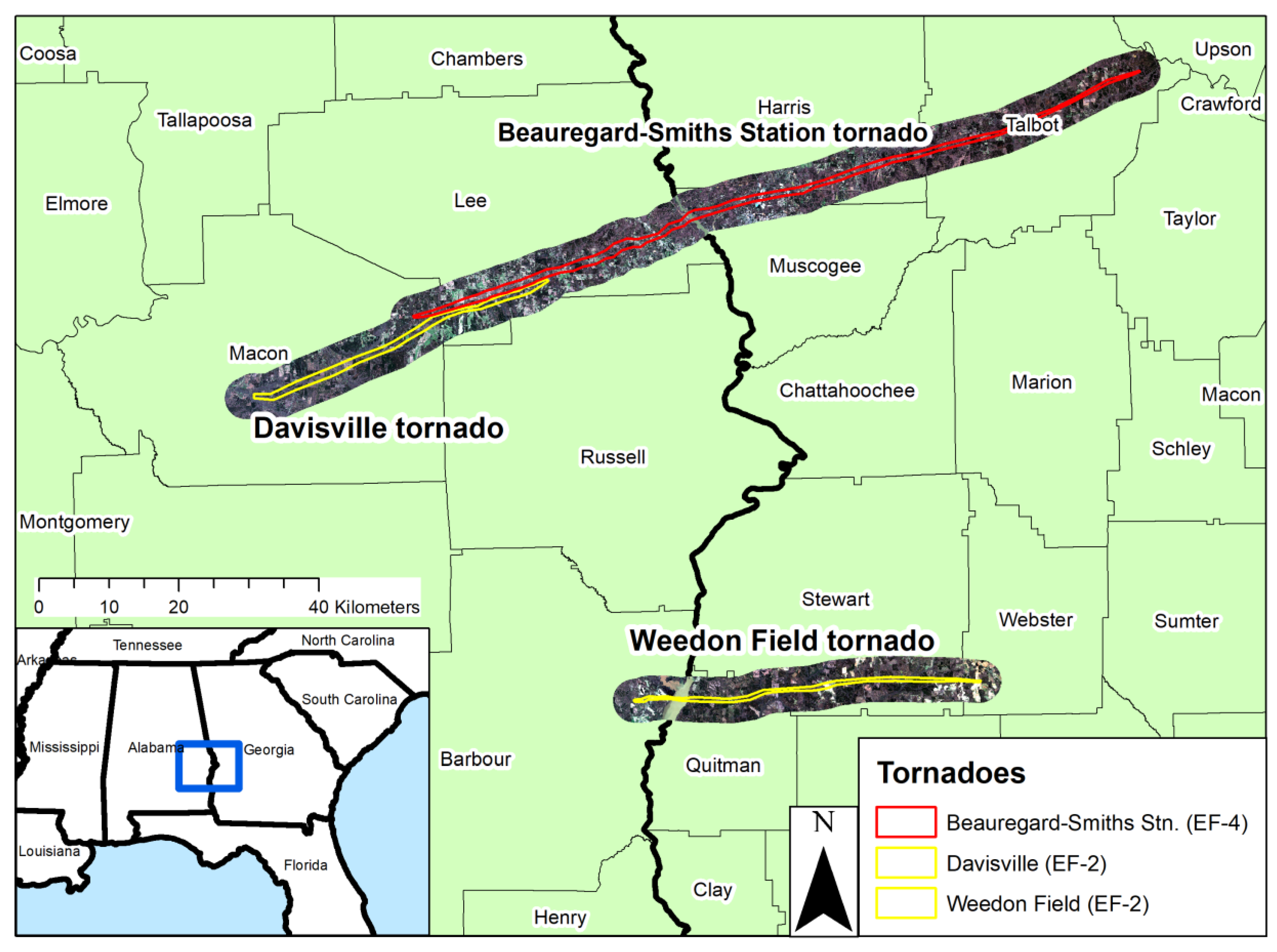
2.1. The 3 March 2019 Tornado Event

An early-season severe weather outbreak occurred across the southeastern United States on 3 March 2019. A total of 40 tornadoes were reported across the region, including an EF-4 that killed 23 people near the community of Beauregard, Alabama [31]. An EF-3 tornado hit Leon County, Florida, just outside of Tallahassee, and seven other EF-2 tornadoes occurred in Alabama, Georgia, and South Carolina. In this study, three tornadoes that occurred on 3 March 2019 were used as case studies. The first tornado of the three devastated Beauregard and Smiths Station, Alabama, at EF-4 intensity before moving over the Chattahoochee River and continuing into Georgia, causing substantial damage in the town of Talbotton. The second tornado was an EF-2 that hit the rural community of Davisville, Alabama, in Macon County, continuing into Lee County and dissipating five miles northwest of Crawford, Alabama. The third tornado included in this study touched down near the Weedon Field airport just north of Eufala, Alabama, crossing the Walter F. George Reservoir into Georgia and affecting mostly rural areas of Quitman, Stewart, and Webster counties. A map of the study area is shown in Figure 1, and further information on these three tornadoes can be found in

Table 1. Damage survey statistics on the three tornadoes analyzed in this study.

Tornado	Maximum Damage Rating	Estimated Peak Wind Speed	Maximum Path Width	Path Length	Time on Ground	Mean Translational Velocity
Beauregard–Smiths Station	EF-4	274 km/h	1465 m	110 km	76 min	86.8 km/h
Davisville	EF-2	185 km/h	1190 m	47 km	30 min	94.0 km/h
Weedon Field	EF-2	209 km/h	785 m	50 km	34 min	88.2 km/h

.

2.2. Data Description

The study region of southeast Alabama and southwest Georgia was well sampled by Sentinel-2 MSI on 24 February 2019, seven days before the tornadoes, and 6 March 2019, three days after the tornadoes, producing > 95% cloud-free images on both dates. The use of imagery from only three days after the event limits the effects of long-term cleanup, post-event vegetation regrowth, etc., on spectral differences between the two images. A majority of the landcover in the region is forested, and the tornadoes occurred early in the growing season. Thus, this event represents ideal conditions for a unique opportunity to study and compare remotely sensed damage patterns between these three strong tornadoes using high-resolution imagery with minimal cloud contamination. Images representing Level-1C geometrically and radiometrically corrected top-of-atmosphere reflectance in the near-infrared and visible red, green, and blue bands were downloaded from the United States Geological Survey (USGS) EarthExplorer website [33]. These bands have central wavelengths at 490 (blue), 560 (green), 665 (red), and 842 (near-infrared) nanometers, each with a spatial resolution of 10 m. Level-1C Sentinel products are registered to subpixel accuracy, and the images used in this study were projected into North American Datum 1983 Universal Transverse Mercator Zone 16N, as appropriate for the longitude of this study region. Using a geographic information system (GIS) platform, each of the images were clipped to a spatial extent representing a three-kilometer buffer around the paths of each tornado, as defined by the surveys conducted by local National Weather Service (NWS) meteorologists. The three-kilometer width of the buffer is about twice the maximum width of the Beauregard–Smiths Station tornado, the widest of the three tornadoes studied here, and allows for spectral patterns of damaged areas to be interpreted in the spatial context of undamaged areas. The landcovers within the tornado damage paths were identified using data from the National Land Cover Database 2016 (NLCD 2016) database. NLCD 2016 is a robust and commonly used data source that identifies land covers across the United States at a 30-m spatial resolution [34].

Data from the NWS Birmingham post-event surveys included 493 damage indicator point locations and estimated wind speeds at those locations. These surveys were performed from 4 March to 7 March 2019, the days immediately following the tornado event. A wide variety of damage indicators were surveyed, including both built and natural features such as trees, agricultural buildings, manufactured homes, and single family residences [31]. Detailed descriptions of the NWS survey process for strong tornadoes can be found in Edwards et al. (2013) [10] and Burgess et al. (2014) [35]. Estimated wind speeds at damage indicators in the NWS Peachtree City survey were not available, so these point locations were not used in this study.

2.3. Normalized Difference Vegetation Index

NDVI was calculated with the red and near-infrared reflectance images from both 24 February and 6 March using Equation (1)

$$\mathrm{NDVI}=\frac{Re{f}_{NIR}-Re{f}_{Red}}{Re{f}_{NIR}+Re{f}_{Red}}$$

(1)

in which $Re{f}_{NIR}$ is the reflectivity of a given pixel in the near-infrared band, and $Re{f}_{Red}$ is the reflectivity of that pixel in the red band. Pixels containing photosynthetically active vegetation are more reflective in near-infrared than in red wavelengths, and thus NDVI is commonly used to measure vegetation health and activity [36]. Pixels containing concentrated healthy vegetation have NDVI values at or above 0.5, while those containing little vegetation have NDVI values near 0.0. The NDVI of water is usually negative. NDVI values from the 24 February image were subtracted from the NDVI value from the 6 March image, creating a new image of NDVI difference. Pixels with negative NDVI values on either 24 February or 6 March were excluded from differencing and further analysis because they were likely dominated by water and thus not useful for detecting damage. Of the $1.344\times {10}^7$ pixels within the tornado path buffers, 2.0% were masked in this manner.

2.4. Principal Components Analysis

The second technique used was a principal component analysis (PCA). PCA is an image enhancement technique that involves an orthogonal transformation of reflectance data into a new set of variables, called principal components, which capture as much variability in the data as possible. While NDVI-differencing uses information from a total of four bands—two bands (red and near-infrared) each on two separate dates (24 February and 6 March)—PCA allows for the addition of more bands into the analysis. The blue and green bands from 24 February and 6 March were included in the PCA, for a total of eight bands. Since PCA is sensitive to extreme values and distributions with uneven scaling, the images were centered and standardized. Pixels with values equal to the mean reflectance in each image were assigned a value of 0.0. Values one standard deviation above and below the mean were assigned the 1.0 and –1.0, respectively, and so on. All eight bands were centered and standardized in this manner before performing the PCA, which produced eight principal component images. This standardization technique has been observed to enhance signal to noise ratio [37] and is used in change detection research to improve results (e.g., [38]).

2.5. Correlating Remotely Sensed Products and Estimated Wind Speeds

To determine the correlations between survey-estimated wind speeds and multispectral indices such as NDVI and PCA, the values of the pixels containing damage indicator locations were obtained from the 6 March NDVI image, the NDVI-difference image (6 March minus 24 February), and the eight principal component images. Then, these pixel values were correlated with the estimated wind speed at that location from the surveys using a simple linear regression for each product.

The two products that had the strongest correlations with estimated wind speeds were NDVI-difference and PC7. From these products, new images were created by applying a square-shaped smoothing window to each pixel in both the NDVI-difference and PC7 image, in which the pixel at the center of the window was reassigned a value equal to the mean of the original values of every pixel in the window. This process was performed using a three-pixel-by-three-pixel (30 m by 30 m) window on the NDVI-difference and PC7 images, and then again using a five-pixel-by-five-pixel (50 m by 50 m) window. This procedure enhanced the correlations between pixel value and estimated wind speed in all four of the new images by reducing statistical noise.

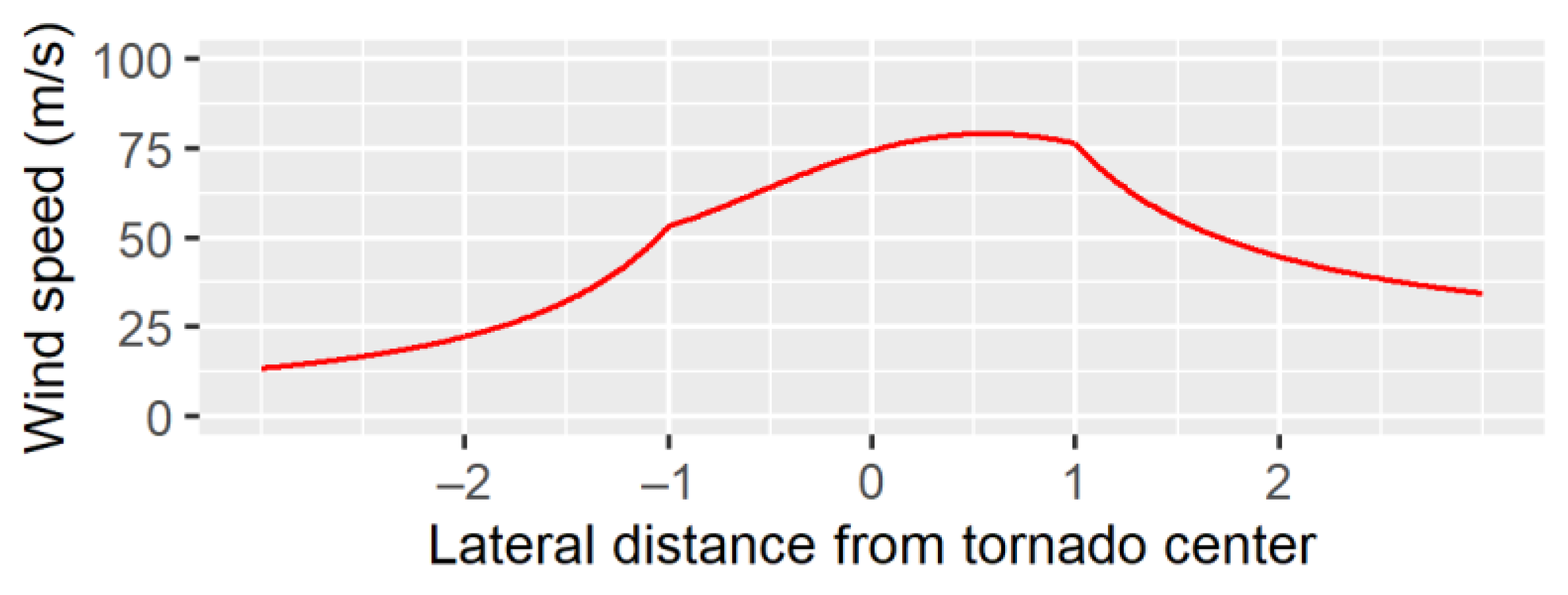
2.6. Evaluating Remotely Sensed Products Across Tornado Widths

The patterns in NDVI difference and PC7 values across the width of each tornado were evaluated by randomly placing 1000 points within the paths of the three tornadoes listed in Table 1. This number of pixels was chosen to ensure sampling throughout the length and width of each tornado path without necessitating the selection of pixels nearby to one another, whose values may be spatially autocorrelated, especially after smoothing windows were applied. The tornado paths were defined by the polygon shapefiles in the NWS Birmingham and NWS Peachtree City storm survey GIS data. The only alterations made to these polygons were to ensure continuity in tornado path width at the Chattahoochee River, which is the boundary between the NWS Birmingham and NWS Peachtree City county warning areas. Values of pixels containing each of the 2000 points placed within the paths of the Davisville and Weedon Field tornadoes were extracted using the NDVI difference and PC7 images created through application of the three-pixel-by-three-pixel smoothing window. The points placed within these two tornado paths were a minimum of 55 m apart to ensure that no two nearby points fell in pixels with values calculated from overlapping smoothing windows. The ratio of sampled pixels to total pixels within the surveyed tornado path was 1:403 for the Davisville tornado and 1:243 for the Weedon Field tornado. This process was repeated in a similar manner for the Beauregard–Smiths Station tornado. Since the Beauregard–Smiths Station tornado path had a much larger area than the other two tornado paths, a larger minimum-distance threshold of 85 m was used for random point placement. This larger minimum-distance threshold allowed for values to be sampled from the NDVI difference and PC7 images created with a five-pixel-by-five-pixel smoothing window, while still ensuring that no two sampled values were calculated from overlapping smoothing windows. The ratio of sampled pixels to total pixels in the Beauregard–Smiths Station tornado path was 1:873.

For each of the three tornadoes, any value from a point that fell in a pixel with a negative NDVI value was excluded from the further analysis, since these pixels were likely water bodies and thus would be inappropriate for estimating tornado wind speeds. This totaled five points in the Beauregard–Smiths Station tornado path, six points in the Davisville tornado path, and fifty-one points in the Weedon Field tornado path, which crossed the Chattahoochee at a wide point in the river. The remaining NDVI-difference and PC7 values were plotted against the distance from the corresponding point to the center of the tornado path. The distances of the points to the left of the tornado path center, relative to storm motion, were multiplied by −1, so that when plotted on a traditional cartesian grid, these points would be separated from points on the right of the path center. The relationship between NDVI difference and point distance from tornado path center, as well as the relationship between PC7 and point distance from tornado path center, were evaluated by fitting a smoothing spline to each of the six plots (NDVI difference and PC7 for each of the three tornadoes). Smoothing splines were used for this purpose because of their flexibility in representing noisy data in which the relationship between dependent and independent variables is not consistent across the domain of independent variables. Since the relationship between wind speed and distance from tornado path center is complex even in basic tornadic wind field models, more simple regressions would not be flexible enough for this purpose. The shapes of these smoothing splines were then compared to the pattern of maximum ground-relative wind speeds across the lateral width of a tornado modelled by a Rankine vortex, such as that shown in Figure 2.

Figure 2 approximates how maximum ground-relative wind speeds vary across the lateral width of a tornado, perpendicular to its translational motion, in a simplistic Rankine vortex model. This figure is used as a template for visual comparison to the distribution of remotely sensed values within the paths of the three tornadoes listed in Table 1. The values in Figure 2 were calculated using the following equations, adapted from those used in Holland et al. (2006), Beck and Dotzek (2010), and Karstens et al. (2013) [26,27,28] and translated to cartesian coordinates

$$V_{gr}=\sqrt{\left(\sin \left(\frac{\pi x}{2R_{max}}\right)\times V_t+\cos \left(\frac{\pi x}{2R_{max}}\right)\times V_r+V_s\right){ }^2+{\left(\cos \left(\frac{\pi x}{2R_{max}}\right)\times V_t-\sin \left(\frac{\pi x}{2R_{max}}\right)\times V_r\right)}^{2 }}$$

(2)

$$V_{gr}=\sqrt{\left(V_t\times R_{max}\times x^{-1}+V_s\right){ }^2+{\left(V_r\times R_{max}\times x^{-1}\right)}^{2 }}$$

(3)

in which $V_t$ is the maximum tangential wind velocity in the vortex, $R_{max}$ is the radius from vortex center at which $V_t$ occurs, $V_r$ is the maximum radial wind velocity towards the center of the vortex, $V_s$ is the translational velocity of the tornado vortex, $x$ is the distance from tornado center measured on a plane oriented perpendicular to its translational vector, and $V_{gr}$ is the approximate maximum ground-relative wind speed at distance $x$. Equation (2) is used when $\left|x\right|$ < $R_{max}$, and Equation (3) is used when $\left|x\right|$ > $R_{max}$. For the purpose of this example, $V_t$ is set to 50 m per second (m/s), $V_r$ to 40 m/s, $V_s$ to 15 m/s, and $R_{max}$ is arbitrarily set to a unitless value of 1.0 in Figure 2, which compares reasonably well to Figure 6 in Karstens et al. (2013) [28] (p. 1055).

To examine the effects of landcover, the 1000 pixels randomly selected from each of the three tornado paths were placed into four different landcover groups depending on the landcover identified at their locations in NLCD 2016. The first group was comprised of forested landcovers, including deciduous forest (class 41), evergreen forest (class 42), mixed forest (class 43), and woody wetlands (class 90). The second group consisted of agricultural landcovers, including pasture/hay (class 81) and cultivated crops (class 82). The third group was comprised of shrubs and grassland, including shrub/scrub (class 52), and grassland/herbaceous (class 71). The fourth group consisted of urban landcovers, including developed open space (class 21), developed low intensity (class 22), developed medium intensity (class 23), and developed high intensity (class 24). Of the 3000 randomly selected pixels, 87 were identified by the NLCD 2016 as other landcover types that were either unlikely to exhibit spectral changes due to tornado damage, including open water (class 11) or barren rock (class 31), or were otherwise not common enough in the study area to draw meaningful conclusions.

3. Results

3.1. Principal Component Analysis of Pre- and Post-Event Imagery

A PCA was performed on eight centered and standardized bands: blue, green, red, and near infrared obtained pre-event on 24 February 2019, and the same four bands obtained post-event on 6 March 2019. The eigenvalues and eigenvectors produced in this analysis are shown in

Table 2. Summary of principal component analysis (PCA) on blue, green, red, and near-infrared bands obtained on 24 February and 6 March.

Value	PC1	PC2	PC3	PC4	PC5	PC6	PC7	PC8
Eigenvalue	0.6119	0.1504	0.0228	0.0115	0.0052	0.0022	0.0014	0.0006
24 Feb Blue Eigenvector	0.3788	0.1464	0.6197	0.0671	0.2880	0.2317	0.5153	0.2108
24 Feb Green Eigenvector	0.3940	0.0514	0.3697	0.1195	−0.5945	0.0019	−0.2114	−0.5414
24 Feb Red Eigenvector	0.3893	0.1018	0.0405	0.7221	−0.0682	0.1185	−0.4721	0.2711
24 Feb NIR Eigenvector	0.2139	−0.6876	0.1580	−0.1006	0.0296	−0.6524	0.0956	0.1040
6 Mar Blue Eigenvector	0.3857	0.1851	−0.1353	0.3959	0.6252	−0.2281	−0.3696	−0.2497
6 Mar Green Eigenvector	0.3912	0.1132	−0.2958	0.4271	−0.3952	−0.0505	−0.0362	0.6358
6 Mar Red Eigenvector	0.3770	0.1929	−0.5357	−0.3122	−0.0461	−0.1303	0.5652	−0.3126
6 Mar NIR Eigenvector	0.2451	−0.6391	−0.2450	0.1143	0.0944	0.6596	−0.0200	−0.1179
Percent variance explained	75.921	18.662	2.825	1.429	0.642	0.273	0.169	0.079

.

Each of the eight principal component images were then correlated with estimated wind speeds at the locations of 493 damage indicators from the NWS Birmingham storm survey. Several of the principal components, such as PC3 and PC6, emphasized differences in reflectance on the two dates, with eigenvalues of opposite signs for the same band on each date.

3.2. Correlating Remotely Sensed Products and Estimated Wind Speeds

The 6 March NDVI, NDVI-difference, and eight PCA values from non-water pixels containing damage indicators from the NWS Birmingham storm survey were then correlated to the estimated wind speeds at those locations to determine which two of these images were the best proxies for damaging tornadic wind speeds. The slopes, intercepts, and ${\mathrm{R}}^2$ values for each of these relationships are listed below in

Table 3. Regression results from normalized difference vegetation index (NDVI) and PCA values as predictors of estimated wind speeds.

Image	Slope	Intercept	${\mathit{R}}^2$Value
6 March NDVI	−0.0011	0.4279	0.0670
6 Mar − 24 Feb NDVI difference	−0.0009	0.0765	0.1040
6 Mar − 24 Feb NDVI difference with 3-by-3 pixel smoothing filter	−0.0011	0.0835	0.2193
6 Mar − 24 Feb NDVI difference with 5-by-5 pixel smoothing filter	−0.0012	0.0898	0.2934
PC1	0.0226	7.7791	0.0131
PC2	0.0024	11.0071	0.0025
PC3	−0.0161	10.0251	0.0574
PC4	0.0071	7.1472	0.0466
PC5	0.0033	5.193	0.0247
PC6	−0.0002	5.2960	0.0003
PC7	0.0044	8.4424	0.1287
PC7 with 3-by-3 pixel smoothing filter	0.0036	8.5236	0.2400
PC7 with 5-by-5 pixel smoothing filter	0.0030	8.5653	0.3021
PC8	−0.0013	15.3674	0.0223

. This table shows that the NDVI-difference and PC7 images exhibited the strongest correlations with estimated wind speeds. Negative NDVI differences within the tornado paths are likely due to vegetation damage, the degree of which is strongly dependent on wind speed. The negative slope in Table 3 indicates that greater vegetation damage is associated with stronger estimated wind speeds. PC7 values also exhibit a relatively strong correlation to estimated wind speeds in the NWS Birmingham survey compared to all other PC values. Smoothing filters were applied to the NDVI-difference and PC7 images, as noted in the Methods section, which increased the correlation strengths by eliminating some statistical noise. These correlations are shown in Table 3, as well. Smoothed NDVI-difference and PC7 images show stronger correlations with estimated wind speeds, as shown by the ${\mathrm{R}}^2$ values that are higher for these images than the others listed in Table 3. Based on these results, the smoothed NDVI-difference and PC7 values were evaluated across the width of the tornado paths.

Visually, remotely sensed signatures consistent with swaths of tornado damage were apparent in many locations within the extent of NWS survey-defined tornado paths. Three examples using post-event NDVI, NDVI-difference, and PC7, the unsmoothed images most strongly correlated with estimated wind speed in Table 2, are shown in Figure 3.

Figure 3a shows 6 March (post-event) NDVI in portions of both the Davisville and Beauregard–Smiths Station tornado paths. The NDVI imagery exhibits patches of both high NDVI in dark green and low NDVI in light green, indicating high and low photosynthetic activity, respectively. The heterogenous landcover in this portion of the study area, a mix between forest and agricultural fields, gives the image its “patchy” look. A faint, elongated region of low NDVI values is visible within the Beauregard–Smiths Station tornado path, in the upper right quadrant of Figure 3a, evidence of reduced vegetative activity due to tornado damage. Figure 3b shows NDVI difference in a portion of intense damage in the Beauregard-Smiths Station tornado path, near the Chattahoochee River. Decreases in NDVI between 24 February and 6 March are evident as dark brown within the NWS survey-defined path of the tornado. Figure 3c shows PC7 values along the Weedon Field tornado path. High PC7 values, correlated with stronger estimated wind speeds in Table 3, are colored in dark brown and exist both inside and outside of the tornado path. This is likely a region of unidentified tornado damage, as will be discussed further. Elongated regions of lighter colored pixels are regions of riparian vegetation, which are detected by PC7 as well.

3.3. Examination of Damage Signatures Across Tornado Path Width

Figure 4, Figure 5 and Figure 6 show how NDVI-difference and PC7 values vary across the lateral width of each of the three tornado paths. Since NDVI decreases are evidence of stronger wind speeds, the NDVI-difference axes have been reversed for easier comparison to Figure 2.

Figure 4 shows the NDVI-difference and PC7 values of pixels containing points placed randomly within the Beauregard–Smiths Station tornado path, plotted in blue. The red lines are smoothing splines fitted with six degrees of freedom. Splines with degrees of freedom varying from two to ten were also fitted to these plots, but the spline with six degrees of freedom for Figure 4a most strongly resembled the curve shown in Figure 2, hence why it is shown here. The spline in Figure 4a, showing NDVI difference, exhibits an absolute minimum at x = 140 m, as well as a relative minimum at x = −120 m (note that the NDVI-difference values on the y-axis have been reversed). The spline shows rapidly increasing NDVI differences at x-values outside of this range. This suggests that the strongest vegetation damage, and inferred strongest wind speeds, occurred within 130 $\pm$ 10 m of the center of the tornado path. Additionally, the shape of the spline in Figure 4a bears a resemblance to the shape of maximum ground-relative wind speeds in Figure 2, which shows quickly decreasing wind speeds outside a radius of $R_{max}$ (1.0 in Figure 2). The smoothing spline in Figure 4b does not exhibit this shape. Although there is a relative maximum in PC7 at about x = 140 m, the shape of the smoothing spline is relatively flat, or even increasing, at values of |x| > 200 m, unlike the shape evident in Figure 2. This suggests that PC7, unlike NDVI difference, is ineffective in this tornado path as a proxy for the wind field pattern in the Rankine vortex, despite the relatively strong correlation with estimated wind speeds at damage indicators in the NWS Birmingham survey (Table 3).

Figure 5 shows the same NDVI-difference and PC7 plots for randomly placed points within the path of the Davisville tornado. The smoothing splines in Figure 5 show little evidence of strong patterns in NDVI difference and PC7 across the width of the Davisville tornado path. These splines have six degrees of freedom for consistency with the smoothing splines in Figure 4, but splines with varying degrees of freedom were fitted to the data and none of them resembled the curve of Figure 2. There is a weak minimum in the Figure 5a spline at x = 100, as well as a weak maximum in Figure 5b at x = 140. These are shown as dashed vertical lines in Figure 5. While the strongest ground-relative wind speeds, and thus the greatest damages, usually occur on the right side of a cyclonically rotating tornado, the smoothing splines in Figure 5 are relatively flat compared to the curve of maximum wind speeds in Figure 2. The remotely sensed damage signature in the Davisville tornado path does not match well with the Rankine vortex model of maximum ground-relative wind speeds using either NDVI difference or PC7. One explanation for this lack of resemblance is that the Davisville tornado was only rated EF2 with peak wind speeds of 185 km/h, which is weaker than the Beauregard Smiths–Station tornado’s peak estimated wind speeds of 284 km/h.

The plots for pixels in the Weedon Field tornado path are shown in Figure 6. The smoothing splines in Figure 6 are relatively flat across the width of the Weedon Field tornado path. Once again, these splines have six degrees of freedom for consistency with Figure 4 and Figure 5, but no spline from these data resembled the shape of the curve in Figure 2, even when the degrees of freedom were adjusted. A weak minimum in NDVI-difference values is evident near the center of the tornado path in Figure 6a, as are marginal increases in NDVI difference and decreases in PC7 (Figure 6b) at distances of |x| > 200 m. However, as in Figure 5, no notable variations in damage in Figure 6 are comparable to the wind field in Figure 2.

3.4. Landcover

Table 4. NDVI-difference and PC7 values of pixels grouped by landcover.

Landcover Group (Tornado)	Number of Pixels	Mean NDVI-Difference Value	Standard Deviation NDVI Difference	Mean PC7 Value	Standard Deviation PC7
Forested (all tornadoes)	2064	0.003	0.032	8.796	0.079
Shrub/grassland (all tornadoes)	495	0.012	0.022	8.779	0.075
Agricultural (all tornadoes)	290	0.020	0.028	8.740	0.126
Urban (all tornadoes)	118	0.004	0.033	8.790	0.091
Forested (Beauregard–Smiths Station)	710	−0.001	0.031	8.820	0.082
Forested (Davisville)	710	0.013	0.025	8.757	0.061
Forested (Weedon Field)	644	−0.004	0.037	8.813	0.077
Shrub/grassland (Beauregard–Smiths Station)	125	0.008	0.026	8.782	0.080
Shrub/grassland (Davisville)	161	0.015	0.022	8.746	0.069
Shrub/grassland (Weedon Field)	209	0.012	0.019	8.803	0.066
Agricultural (Beauregard-Smiths Station)	77	0.017	0.028	8.787	0.100
Agricultural (Davisville)	90	0.025	0.020	8.715	0.080
Agricultural (Weedon Field)	123	0.018	0.032	8.730	0.159
Urban (Beauregard–Smiths Station)	59	0.004	0.028	8.789	0.084
Urban (Davisville)	31	0.014	0.028	8.758	0.076
Urban (Weedon Field)	28	−0.010	0.041	8.827	0.105

shows the NDVI difference and PC7 values of the randomly selected pixels in each of the three tornado paths, categorized into four groups of similar landcover classes in NLCD 2016, as described in the Methods section. Mean NDVI-difference values tend to be most negative in forested and urban landcover groups. PC7 values are highest for these landcover groups as well. The shrub/grassland and agricultural landcover groups exhibit the highest NDVI-difference and lowest PC7 values. However, variance is relatively high, and the differences between the forested and agricultural landcover groups are greater in magnitude than the standard deviations of either of these groups.

3.5. A region of Displacement between the Survey-Defined Tornado Path and NDVI Decrease

While the tornado-path polygons produced in the post-event surveys [30,31] matched the remotely sensed damage areas from this study quite well, one region of apparent displacement was located in southern Stewart County and northern Quitman County, Georgia, shown in Figure 7. The brown pattern below (to the south of) the survey-defined tornado path in Figure 7 is an area of NDVI decrease, indicating vegetation damage, between 24 February and 6 March. This region runs parallel one kilometer to the south of the survey-defined tornado path for a distance of about five kilometers along it, or about one-tenth the length of the Weedon Field tornado path. This was the only portion of the three tornado paths that exhibited an elongated spatial displacement between apparent damage and the path polygons themselves, so displacement between the remotely sensed damage signatures and survey-defined paths is unlikely to substantially compromise the results shown in Figure 4, Figure 5 and Figure 6.

4. Discussion

Results in Table 3 show that NDVI differencing and PCA are effective in identifying areas of tornado damage and approximating damage intensity. However, neither product is without its drawbacks. NDVI differencing is less effective outside the growing season or in regions with little vegetation, as several studies have noted [17,18,19,21]. The relative lack of damage indicators for vegetation [10] may mean that the intensities of these tornadoes were underestimated in forested areas, where NDVI decreases are most pronounced (Table 4). A comparison of NDVI difference and EF-scale damage estimates in forested areas (e.g., [11]) would shed light on this problem. The interpretation of PCA varies by study area, band inclusion, and other factors, and is thus difficult to compare from one event to the other, despite favorable results in this study and others [14,19,20].

The correlations of both PCA and NDVI-difference values with estimated wind speeds were improved by a smoothing window, which served to dampen noise in the reflectance data. While high-resolution imagery provides more detail on damage patterns than imagery from lower-resolution sensors [14], the positive results obtained through use of the smoothing window suggest that substantial variability in the reflectance of neighboring pixels in high-resolution imagery presents a challenge in estimating wind speeds over small spatial scales. A hypothetical example of this would be in a low-density residential region. A pixel comprised of reflectance from a non-vegetated surface like a house would be unlikely to exhibit a substantial decrease in NDVI due to tornado damage. However, neighboring pixels comprised of vegetated surfaces such as lawns and suburban tree cover would exhibit stronger decreases in NDVI as this vegetation is damaged by the tornado or covered in debris. The pixel containing reflectance from the house would have its NDVI-difference value decreased by a smoothing window that includes NDVI decreases in neighboring vegetated pixels, more accurately reflecting strong wind speeds.

Another notable finding in this study is the high eigenvector magnitude on the blue bands in PC7 (Table 2) and the relatively strong correlation between PC7 and estimated tornadic wind speeds (Table 3) compared to other PCs. For the 24 February image, blue reflectance has a positive PC7 eigenvector, and red reflectance has a negative eigenvector. However, for the 6 March image, blue reflectance has a negative eigenvector, while red reflectance has a positive eigenvector. This means that pixels exhibiting a higher ratio of red reflectance to blue reflectance on 6 March than on 24 February will have high PC7 values, which are correlated to stronger wind speeds in Table 3. For example, a pixel dominated by vegetation in the 24 February image will have a nearly even ratio of red to blue reflectance because vegetation reflects at a similar rate in these wavelengths. If vegetation in that pixel is damaged by a tornado, exposing soil beneath, the ratio of red to blue reflectance will increase because soil is more reflective in red wavelengths than in blue wavelengths. As a result, this pixel would register a high PC7 value given the eigenvectors in Table 2, indicating strong winds at that location (Table 3). Some previous studies that used PCA to delineate tornado paths did not include blue reflectance in the analysis, either because the sensor of choice did not obtain blue reflectance data [19], or for the sake of consistency with previous research [14]. While these are logical reasons for the omission of blue reflectance, including it in either PCA or other multispectral indices may be beneficial to future studies like this one.

The similarity between the smoothing spline of NDVI difference across the width of the Beauregard–Smiths Station tornado path (Figure 4a) to the pattern of maximum ground-relative wind speeds across the width of a tornado in a Rankine vortex model (Figure 2) is another intriguing finding of this study. NDVI-difference values reached minima, indicating strong vegetation damage, at distances of 130 ± 10 m on both sides of the center of the tornado path in Figure 6a. This distance may serve as a starting point for an estimation of $R_{max}$, although it should be noted that direct estimates of $R_{max}$ using radar data can differ from the width of maximum on-the-ground damage [39]. Empirical calculations of $V_t$ and $V_r$ in Equations (2) and (3) are difficult, requiring the use of high-resolution tree fall data [26,27,28,40], and are not likely feasible using NDVI-difference products at a 10-m resolution. Surprisingly, a signature similar to Figure 2 was not apparent in the PC7 values in the Beauregard–Smiths Station tornado path (Figure 4b), despite their relatively strong correlation to estimated wind speeds in the NWS Birmingham survey (Table 2). A maximum in the smoothing spline of PC7 values, indicating stronger wind speeds, was located at 140 m to the right of the tornado path center, but a strong decrease in PC7 values was not evident in the outer flanks of the path. The reasons for this are unclear, but perhaps small-scale variations in tornadic wind fields are best proxied by indices that detect vegetation damage, such as NDVI, rather than PCA techniques that might be affected by other unrelated factors. Yuan et al. (2002) suggested that NDVI differencing outperforms PCA in detecting areas of F2 (the Enhanced Fujita scale was not yet implemented at the time the study was published) and F1 damage [19]. It is possible that the NDVI-differencing technique replicates damage patterns resembling the Rankine vortex wind field in Figure 2 because it is more sensitive specifically to relatively weak damage, which is likely to be found near the exterior of the tornado path. If this is the case, detecting a damage signature consistent with the wind field in Figure 2 requires both intense tornado damage and a spectral index that is sufficiently sensitive to weaker damage as well.

The Davisville and Weedon Field tornadoes did not exhibit patterns in NDVI differences or PC7 values consistent with the Rankine vortex wind field in Figure 2. This is probably attributable to their weaker intensities (Table 1). Even in violent tornadoes, the strongest wind speeds usually encompass only a fraction of the tornado path [35,41,42], and regions of greatest vegetation damage are often confined to small areas [15]. NDVI differencing becomes much less effective at detecting tornado damage at < EF2 intensities [14,19,21]. The Davisville and Weedon Field tornadoes likely did not produce sufficiently intense damage over large enough areas for the randomly sampled pixels in Figure 4 and Figure 5 to show substantial variation in NDVI difference and PC7 across the width of the tornado paths.

Variations in landcover within the tornado paths may also play a role in masking the relationship between multispectral indices and damage. While a detailed examination of damage signatures in various landcovers is outside the scope of this study, Table 4 suggests that damage tends to be more evident in regions of forested and urban landcovers. Forested areas are comprised of dense vegetation, and vegetation indices such as NDVI are particularly effective for identifying vegetation damage [17]. Of the 118 pixels in urban areas (Table 4), 113 (96 percent) were classified in NLCD 2016 as either “Developed, open space” or “Developed, low intensity”, which are both classes in which lawn grasses and trees may comprise a substantial portion of cover. As such, NDVI and other vegetation indices can still be effective in detecting damage to this vegetation. The destruction of houses and other buildings found in urban areas also produces large amounts of debris, and regions of extensive debris coverage are easily detectable using multispectral methods [19]. Further analysis of the relationship between landcover and high -resolution damage detection (e.g., [18]) is an opportunity for further study.

Image selection is another notable factor for consideration of the results presented here. Molthan et al. (2014) found that NDVI decreases in the weeks following a tornado became marginally more pronounced with increases in EF-scale damage, but variance was relatively high within each damage level [14]. The authors suggested that non-meteorological processes such as cleanup efforts are likely the cause of these NDVI decreases [14]. Thus, detailed post-event damage analysis should ideally be conducted with imagery obtained as soon as possible after the event, since non-meteorological processes that inevitably occur in the days after the event affect the landscape in complex ways that might mask fine-scale variations in damage. This may especially be true in urban areas, where anthropogenic activities are most concentrated. While some cleanup undoubtedly occurred in the days immediately following the tornadoes examined in this study, the three-day lag between the tornado event (3 March 2019) and the post-event image used for analysis (obtained on 6 March 2019) compares well with similar studies such as Yuan et al. (2002) (five days), Molthan et al. (2014) (three to seven days or more, sensor dependent), and Myint et al. (2008) (nine days) [14,19,20]. Kingfield and de Beurs (2017) provided a detailed exploration of vegetation recovery in the five years following the 27 April 2011 tornado outbreak using Landsat imagery, finding that substantial recovery, relative to nearby undamaged regions, did not begin until six months after the event [18]. Future studies could conduct a similar examination of short- and medium-term reflectance changes in damaged areas over small spatial scales, as this could shed light on the importance of data latency in post-event image selection.

An advantage of this study’s methods is in their ease of being replicable. Detailed studies of tornado damage using aerial imagery often involve manual inspection and tree fall digitization [11,27,28], which produce very detailed datasets, but are also very time intensive and require aerial imagery of the affected area, which can be expensive to obtain. NDVI, on the other hand, is a very common metric in the Earth observation literature and is easy to calculate at the expense of some level of detail. Imagery obtained from UAVs and satellites with a very fine (< 10-m) spatial resolution will increasingly be used for future damage assessments of this nature [12,13,43,44].

This approach can also be used to refine ground-based damage surveys. One example of this is the region of displacement between NDVI decreases and the survey-defined path polygon shown in Figure 7. Such displacement between remotely sensed damage and ground-level surveys, especially perpendicular to storm motion, is not uncommon in rural regions [14,16,45]. While Karstens et al. (2013) [28] noted tree falls associated with rear flank downdraft (RFD) surges to the right of the 22 May 2011 Joplin, Missouri, tornado track, these surges caused substantially less damage than was found within the path of the Joplin tornado. Given the severity of the damage shown in Figure 7 outside of the path relative to the damage inside it, Figure 7 likely shows damage from the tornado itself that was not included in the survey-defined path because it would have been nearly impossible for surveyors to notice or access from ground level.

5. Conclusions

This study examines damage from three tornadoes using imagery from Sentinel-2 MSI with a 10-m spatial resolution. Pixel values from post-event NDVI, NDVI differences, and eight principal component images are correlated with estimated wind speeds at damage indicators noted in post-event surveys. The strongest correlations with these wind speeds are in the NDVI-difference image and one of the principal component images (PC7), after applying a five-pixel-by-five-pixel filter window to each image to diminish statistical noise. Random points are then placed within each of the three tornado paths, and NDVI-difference and PC7 values at the location of these points are plotted against the distance from each respective point to the center of the tornado path. The shape of a smoothing spline fitted to the NDVI-difference values in the Beauregard–Smiths Station tornado path resembles the pattern of ground-relative maximum wind speeds across the width of a tornado in the Rankine vortex model. The most intense damage detected with these methods occurred within 130 m of the tornado path center, which may serve as a rough estimate for $R_{max}$ for this tornado. However, the shapes of the smoothing splines fitted to PC7 values in the Beauregard–Smiths Station tornado, as well as both NDVI-difference and PC7 values in the weaker Davisville and Weedon Field tornadoes, are relatively flat across the width of the tornado paths. It is concluded that, with little cloud contamination, imagery with ≤ 10-m spatial resolution such as that from Sentinel-2 MSI can be used to approximate damage intensity of vegetated areas and fine-tune the extent of tornado paths delineated in on-the-ground surveys. Pixel-level atmospheric corrections may be able to provide even more detail on ground-level damage patterns, as may UAV imagery, which is obtained from a low altitude [13]. The techniques and findings presented in this study may be of value to future research on vegetative response to tornado damage (e.g., [1,11,18]), as well as comparisons between ground surveys, radar observations, and passively sensed imagery (e.g., [12,16,35,39,42,46]). As high-resolution UAV and satellite imagery becomes increasingly available, these multi-platform studies will be able to make detailed observations of tornado dynamics to aid advances in modeling, building safety, and similar efforts.

References

1. Peterson, C.J.; Rebertus, A.J. Tornado damage and initial recovery in three adjacent, lowland temperate forests in Missouri. J. Veg. Sci. 1997, 8, 559–564. [Google Scholar] [CrossRef]
2. Peterson, C.J. Consistent influence of tree diameter and species on damage in nine eastern North America tornado blowdowns. For. Ecol. Manag. 2007, 250, 96–108. [Google Scholar] [CrossRef]
3. Gutter, B.; Brown, M.; Cox, D.A. Investigation of Vegetation Discontinuities Related to the Yazoo City Tornado Scar and Enhanced Convection. J. Geol. Geosci. 2015, 4, 185. [Google Scholar] [CrossRef]
4. White, S.D.; Hart, J.L.; Schweitzer, C.J.; Dey, D.C. Altered structural development and accelerated succession from intermediate-scale wind disturbance in Quercus stands on the Cumberland Plateau, USA. For. Ecol. Manag. 2015, 336, 52–64. [Google Scholar] [CrossRef]
5. Trammell, B.W.; Hart, J.L.; Schweitzer, C.J.; Dey, D.C.; Steinberg, M.K. Effects of intermediate-severity disturbance on composition and structure in mixed Pinus-hardwood stands. For. Ecol. Manag. 2017, 400, 110–122. [Google Scholar] [CrossRef]
6. Gallo, K.; Smith, T.; Jungbluth, K.; Schumacher, P. Hail Swaths Observed from Satellite Data and Their Relation to Radar and Surface-Based Observations: A Case Study from Iowa in 2009. Weather Forecast. 2012, 27, 796–802. [Google Scholar] [CrossRef]
7. Gallo, K.; Schumacher, P.; Boustead, J.; Ferguson, A. Validation of Satellite Observations of Storm Damage to Cropland with Digital Photographs. Weather Forecast. 2019, 34, 435–446. [Google Scholar] [CrossRef]
8. Fujita, T.; Bradbury, D.; Van Thullenar, C.F. Palm Sunday tornadoes of April 11, 1965. Mon. Weather. Rev. 1970, 98, 29–69. [Google Scholar] [CrossRef]
9. Davies-Jones, R.; Burgess, D.; Lemon, L.; Purcell, D. Interpretation of surface marks and debris pattern from the 24 May 1973 Union City, Oklahoma tornado. Mon. Weather Rev. 1978, 106, 12–21. [Google Scholar] [CrossRef] [Green Version]
10. Edwards, R.; LaDue, J.G.; Ferree, J.T.; Scharfenberg, K.; Maier, C.; Coulbourne, W.L. Tornado Intensity Estimation: Past, Present, and Future. Bull. Amer. Meteor. Soc. 2013, 94, 641–653. [Google Scholar] [CrossRef]
11. Godfrey, C.M.; Peterson, C.J. Estimating Enhanced Fujita Scale Levels Based on Forest Damage Severity. Weather Forecast. 2016, 32, 243–252. [Google Scholar] [CrossRef]
12. Womble, J.A.; Wood, R.L.; Mohammadi, M.E. Multi-scale remote sensing of tornado effects. Front. Built Environ. 2018, 4, 1–21. [Google Scholar] [CrossRef]
13. Wagner, M.; Doe, R.K.; Johnson, A.; Chen, Z.; Das, J.; Cerveny, R.S. Unpiloted Aerial Systems (UASs) Application for Tornado Damage Surveys: Benefits and Procedures. Bull. Am. Meteor. Soc. 2019, 100, 2405–2409. [Google Scholar] [CrossRef]
14. Molthan, A.; Bell, J.; Cole, T.; Burks, J. Satellite-based identification of tornado damage tracks from the 27 April 2011 severe weather outbreak. J. Operational Meteor. 2014, 2, 191–208. [Google Scholar] [CrossRef]
15. Cannon, J.B.; Hepinstall-Cymerman, J.; Godfrey, C.M.; Peterson, C.J. Landscape-scale characteristics of forest tornado damage in mountainous terrain. Landsc. Ecol. 2016, 31, 2097–2114. [Google Scholar] [CrossRef]
16. Lyza, A.W.; Castro, R.; Lenning, E.; Friedlein, M.T.; Borchardt, B.S.; Clayton, A.W.; Knupp, K.R. A Multi-Platform Reanalysis of the Kankakee Valley Tornado Cluster on 30 June 2014. Electron. J. Sev. Storms Metereol. (EJSSM) 2019, 14, 1–64. [Google Scholar]
17. Jedlovec, G.J.; Nair, U.; Haines, S.L. Detection of Storm Damage Tracks with EOS Data. Weather Forecast. 2006, 21, 249–267. [Google Scholar] [CrossRef]
18. Kingfield, D.M.; de Beurs, K.M. Landsat Identification of Tornado Damage by Land Cover and an Evaluation of Damage Recovery in Forests. J. Appl. Meteor. Climatol. 2017, 56, 965–987. [Google Scholar] [CrossRef]
19. Yuan, M.; Dickens-Micozzi, M.; Magsig, M.A. Analysis of Tornado Damage Tracks from the 3 May Tornado Outbreak Using Multispectral Satellite Imagery. Weather Forecast. 2002, 17, 382–398. [Google Scholar] [CrossRef]
20. Myint, S.W.; Yuan, M.; Cerveny, R.S.; Giri, C.P. Comparison of Remote Sensing Image Processing Techniques to Identify Tornado Damage Areas from Landsat TM Data. Sensors 2008, 8, 1128–1156. [Google Scholar] [CrossRef] [PubMed] [Green Version]
21. Burow, D.; Rundquist, B.; Atkinson, C. NDVI change analysis and damage mapping of the Vilonia, Arkansas tornado, 27 April 2014. Pap. Appl. Geogr. 2017, 3, 85–100. [Google Scholar] [CrossRef]
22. Peterson, R.E. Johannes Letzmann: A Pioneer in the Study of Tornadoes. Weather Forecast. 1992, 7, 166–184. [Google Scholar] [CrossRef] [Green Version]
23. Wood, V.T.; White, L.W. A New Parametric Model of Vortex Tangential-Wind Profiles: Development, Testing, and Verification. J. Atmos. Sci. 2011, 68, 990–1006. [Google Scholar] [CrossRef]
24. Wood, V.T.; White, L.W. A Parametric Wind–Pressure Relationship for Rankine versus Non-Rankine Cyclostrophic Vortices. J. Atmos. Oceanic Technol. 2013, 30, 2850–2867. [Google Scholar] [CrossRef] [Green Version]
25. Kim, Y.C.; Matsui, M. Analytical and empirical models of tornado vortices: A comparative study. J. Wind Eng. Ind. Aerodyn. 2017, 171, 230–247. [Google Scholar] [CrossRef]
26. Holland, A.P.; Riordan, A.J.; Franklin, E.C. A Simple Model for Simulating Tornado Damage in Forests. J. Appl. Meteor. Climatol. 2006, 45, 1597–1611. [Google Scholar] [CrossRef]
27. Beck, V.; Dotzek, N. Reconstruction of Near-Surface Tornado Wind Fields from Forest Damage. J. Appl. Meteor. Climatol. 2010, 49, 1517–1537. [Google Scholar] [CrossRef] [Green Version]
28. Karstens, C.D.; Gallus, W.A.; Lee, B.D.; Finley, C.A. Analysis of Tornado-Induced Tree Fall Using Aerial Photography from the Joplin, Missouri, and Tuscaloosa–Birmingham, Alabama, Tornadoes of 2011. J. Appl. Meteor. Climatol. 2013, 52, 1049–1068. [Google Scholar] [CrossRef] [Green Version]
29. Strader, S.M.; Ashley, W.; Irizarry, A.; Hall, S. A climatology of tornado intensity assessments. Meteorol. Appl. 2015, 22, 513–524. [Google Scholar] [CrossRef]
30. National Weather Service Peachtree City. March 3, 2019 Tornadoes. Available online: https://www.weather.gov/ffc/20190303_tornadoes (accessed on 26 February 2020).
31. National Weather Service Birmingham. Tornadoes of March 3, 2019. Available online: https://www.weather.gov/bmx/event_03032019 (accessed on 26 February 2020).
32. Roueche, D.; Prevatt, D. Residential Damage Patterns Following the 2011 Tuscaloosa, AL and Joplin, MO Tornadoes. J. Disaster Res. 2013, 8, 1061–1067. [Google Scholar] [CrossRef]
33. United States Geological Survey. EarthExplorer. Available online: https://earthexplorer.usgs.gov/ (accessed on 9 June 2020).
34. Yang, L.; Jin, S.; Danielson, P.; Homer, C.; Gass, L.; Bender, S.M.; Case, A.; Costello, C.; Dewitz, J.; Fry, J.; et al. A new generation of the United States National Land Cover Database: Requirements, research priorities, design, and implementation strategies. ISPRS J. Photogramm. Remote Sens. 2018, 146, 108–123. [Google Scholar] [CrossRef]
35. Burgess, D.; Ortega, K.; Stumpf, G.; Garfield, G.; Karstens, C.; Meyer, T.; Smith, B.; Speheger, D.; Ladue, J.; Smith, R.; et al. 20 May 2013 Moore, Oklahoma, Tornado: Damage Survey and Analysis. Weather Forecast. 2014, 29, 1229–1237. [Google Scholar] [CrossRef]
36. Pettorelli, N.; Vik, J.O.; Mysterud, A.; Gaillard, J.-M.; Tucker, C.J.; Stenseth, N.C. Using the satellite-derived NDVI to assess ecological responses to environmental change. Trends Ecol. Evol. 2005, 20, 503–510. [Google Scholar] [CrossRef] [PubMed]
37. Singh, A.; Harrison, A. Standardized principal components. Int. J. Remote Sens. 1985, 6, 883–896. [Google Scholar] [CrossRef]
38. Li, X.; Yeh, A.G.O. Principal component analysis of stacked multi-temporal images for the monitoring of rapid urban expansion in the Pearl River Delta. Int. J. Remote Sens. 1998, 19, 1501–1518. [Google Scholar] [CrossRef]
39. Wurman, J.; Alexander, C.R. The 30 May 1998 Spencer, South Dakota, Storm. Part II: Comparison of Observed Damage and Radar-Derived Winds in the Tornadoes. Mon. Wea. Rev. 2005, 133, 97–119. [Google Scholar] [CrossRef]
40. Chen, G.; Lombardo, F.T. An analytical pattern-based method for estimation of a near-surface tornadic wind field. J. Wind Eng. Industrial Aerodyn. 2019, 194, 103999. [Google Scholar] [CrossRef]
41. Speheger, D.A.; Doswell, C.A.; Stumpf, G.J. The Tornadoes of 3 May 1999: Event Verification in Central Oklahoma and Related Issues. Weather Forecast. 2002, 17, 362–381. [Google Scholar] [CrossRef] [Green Version]
42. Atkins, N.T.; Butler, K.M.; Flynn, K.R.; Wakimoto, R.M. An Integrated Damage, Visual, and Radar Analysis of the 2013 Moore, Oklahoma, EF5 Tornado. Bull. Am. Meteor. Soc. 2014, 95, 1549–1561. [Google Scholar] [CrossRef]
43. Molthan, A.L.; Schultz, L.A.; McGrath, K.M.; Burks, J.E.; Camp, J.P.; Angle, K.; Bell, J.R.; Jedlovec, G.J. Incorporation and Use of Earth Remote Sensing Imagery within the NOAA/NWS Damage Assessment Toolkit. Bull. Amer. Meteor. Soc. 2019. BAMS-D-19-0097.1. [Google Scholar] [CrossRef] [PubMed]
44. Kakooei, M.; Baleghi, Y. Fusion of satellite, aircraft, and UAV data for automatic disaster damage assessment. Int. J. Remote Sens. 2017, 38, 2511–2534. [Google Scholar] [CrossRef]
45. Shikhov, A.; Chernokulsky, A. A satellite-derived climatology of unreported tornadoes in forested regions of northeast Europe. Remote Sens. Environ. 2018, 204, 553–567. [Google Scholar] [CrossRef]
46. Skow, K.D.; Cogil, C. A High-Resolution Aerial Survey and Radar Analysis of Quasi-Linear Convective System Surface Vortex Damage Paths from 31 August 2014. Weather Forecast. 2016, 32, 441–467. [Google Scholar] [CrossRef]
Figure 1. Study area with tornado paths outlined over RGB composite images obtained by Sentinel-2 MSI on 6 March 2019.
Atmosphere 11 00613 g001
Figure 2. Approximation of how maximum ground-relative wind speeds vary across the lateral width of a tornado in the Rankine vortex model.
Atmosphere 11 00613 g002
Figure 3. Close-up of remotely sensed damage signatures using three different metrics: (a) Post-event NDVI measured on 6 March, (b) NDVI difference, and (c) PC7. (d) Shows the extent of (ac) within the tornado paths.
Atmosphere 11 00613 g003
Figure 4. Values of pixels containing randomly placed points within the Beauregard–Smiths Station tornado path, plotted by distance from tornado center: (a) NDVI difference between 6 March and 24 February, and (b) Principal Component 7. The dashed vertical line represents the lateral distance from tornado center corresponding to the relative minimum (a) and maximum (b) in the smoothing spline. The grey-shaded envelope represents the 95% confidence interval of the smoothing spline values.
Atmosphere 11 00613 g004
Figure 5. Values of pixels containing randomly placed points within the Davisville tornado path, plotted by distance from tornado center: (a) NDVI difference between 6 March and 24 February, and (b) Principal Component 7. The dashed vertical line represents the lateral distance from the tornado center corresponding to the relative minimum (a) and maximum (b) in the smoothing spline. The grey-shaded envelope represents the 95% confidence interval of smoothing spline values.
Atmosphere 11 00613 g005
Figure 6. Values of pixels containing randomly placed points within the Weedon Field tornado path, plotted by distance from tornado center: (a) NDVI difference between 6 March and 24 February, and (b) Principal Component 7. The grey-shaded envelope represents the 95-percent confidence interval of smoothing spline values.
Atmosphere 11 00613 g006
Figure 7. Region of displacement between surveyed path extent and remotely sensed vegetation damage.
Atmosphere 11 00613 g007