Atmospheric Aerosol Distribution in 2016–2017 over the Eastern European Region Based on the GEOS-Chem Model

 ,
, 

Abstract
:1. Introduction
2. Materials and Methods
3. Results
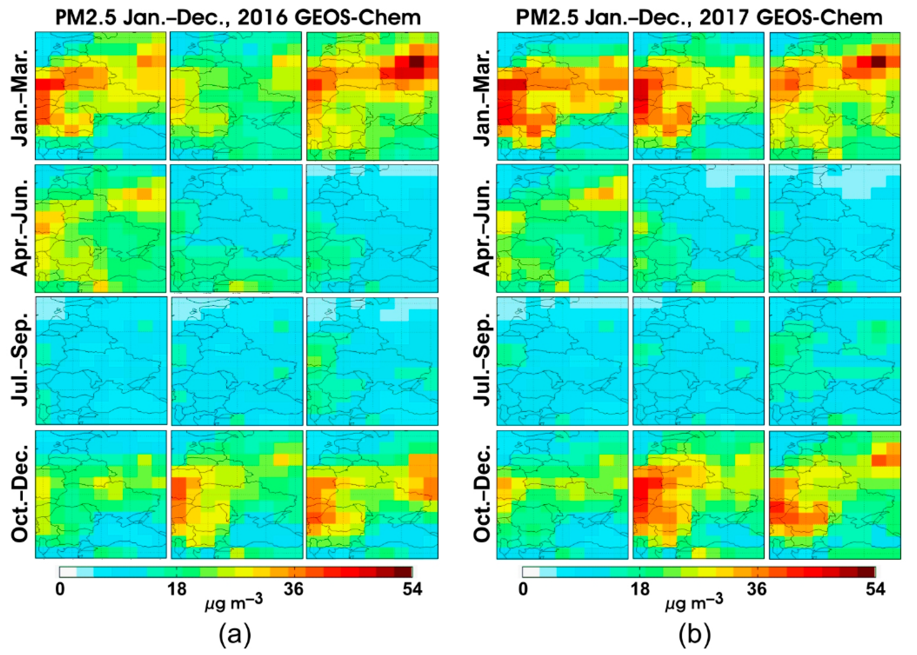
3.1. PM2.5
3.2. Mineral Dust
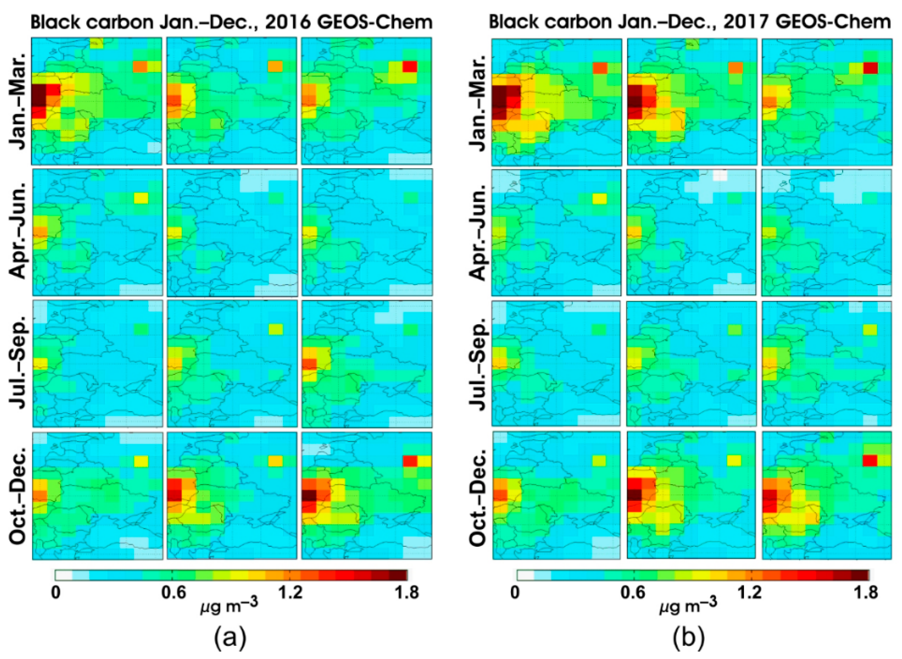
3.3. Black Carbon
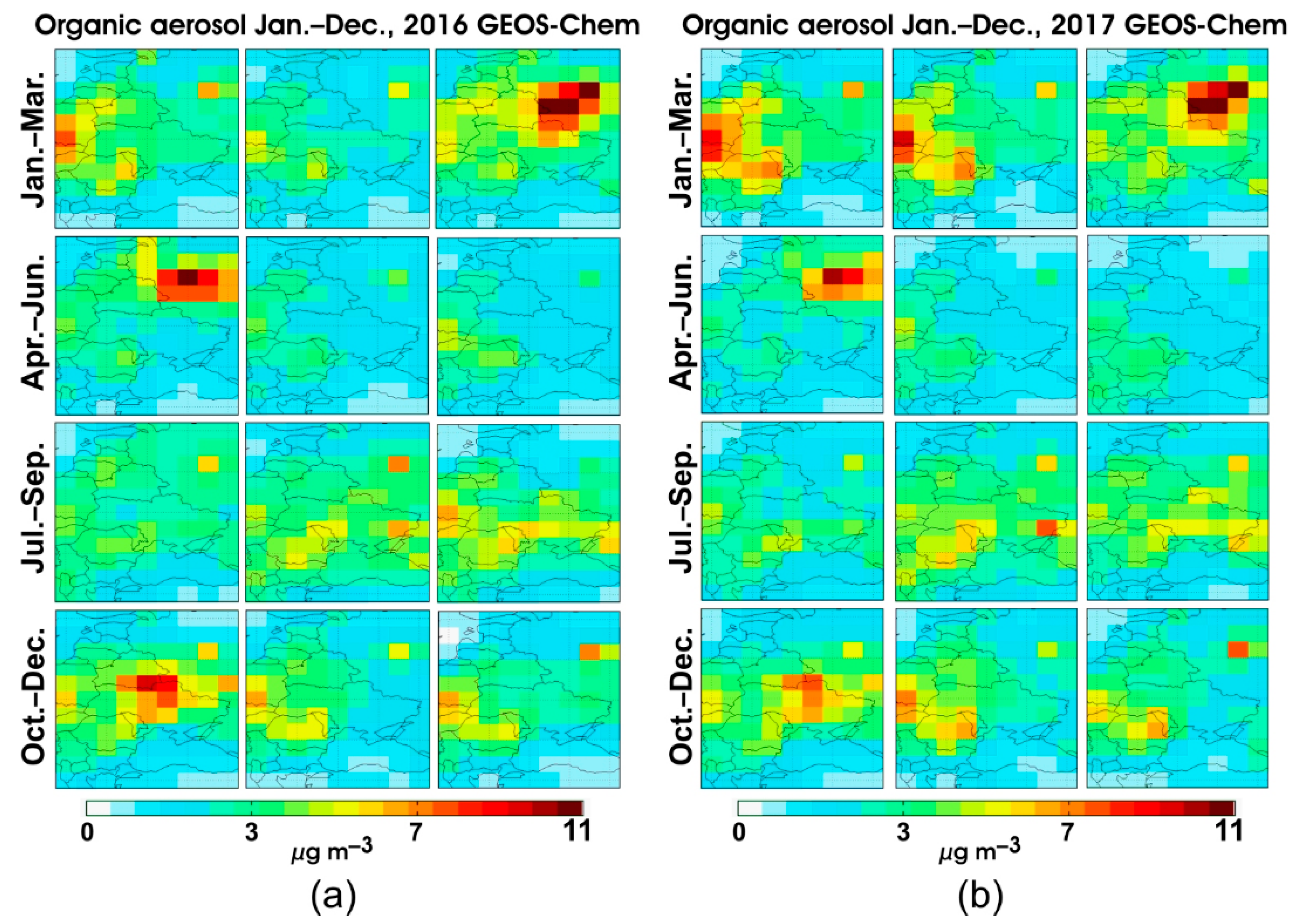
3.4. Organic Aerosols
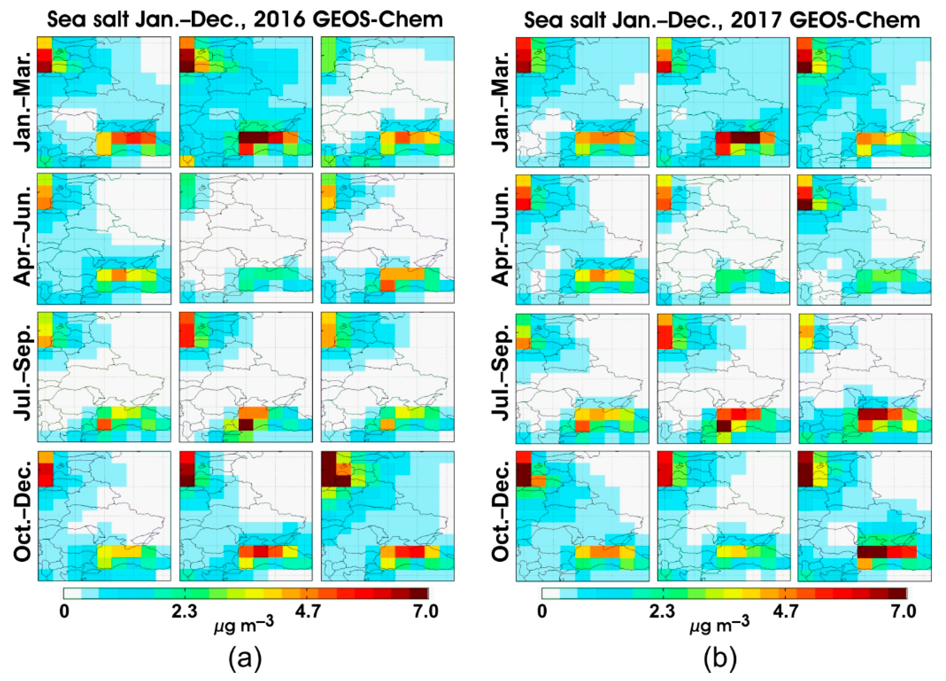
3.5. Sea Salt
3.6. Nitrate, Sulfate, and Ammonium Aerosols
4. Discussion
5. Conclusions
Author Contributions
Funding
Acknowledgments
Conflicts of Interest
References
- Tzanis, C.; Varotsos, C.A. Tropospheric aerosol forcing of climate: A case study for the greater area of Greece. Int. J. Remote Sens. 2008, 29, 2507–2517. [Google Scholar] [CrossRef]
- Hartmann, D.L.; Klein Tank, A.M.G.; Rusticucci, M.; Alexander, L.V.; Brönnimann, S.; Charabi, Y.; Dentener, F.J.; Dlugokencky, E.J.; Easterling, D.R.; Kaplan, A.; et al. Observations: Atmosphere and surface. In Climate Change 2013: The Physical Science Basis. Contribution of Working Group I to the Fifth Assessment Report of the Intergovernmental Panel on Climate Change; Stocker, T.F., Qin, D., Plattner, G.-K., Tignor, M., Allen, S.K., Boschung, J., Nauels, A., Xia, Y., Bex, V., Midgley, P.M., Eds.; Cambridge University Press: Cambridge, UK; New York, NY, USA, 2013. [Google Scholar]
- Derimian, Y.; Dubovik, O.; Huang, X.; Lapyonok, T.; Litvinov, P.; Kostinski, A.B.; Dubuisson, P.; Ducos, F. Comprehensive tool for calculation of radiative fluxes: Illustration of shortwave aerosol radiative effect sensitivities to the details in aerosol and underlying surface characteristics. Atmos. Chem. Phys. 2016, 16, 5763–5780. [Google Scholar] [CrossRef] [Green Version]
- Holben, B.N.; Eck, T.F.; Slutsker, I.; Tanré, D.; Buis, J.P.; Setzer, A.; Vermote, E.; Reagan, J.A.; Kaufman, Y.J.; Nakajima, T.; et al. AERONET—A federated instrument network and data archive for aerosol characterization. Remote Sens. Environ. 1998, 66, 1–16. [Google Scholar] [CrossRef]
- Holben, B.N.; Kim, J.; Sano, I.; Mukai, S.; Eck, T.F.; Giles, D.M.; Schafer, J.S.; Sinyuk, A.; Slutsker, I.; Smirnov, A.; et al. An overview of mesoscale aerosol processes, comparisons, and validation studies from DRAGON networks. Atmos. Chem. Phys. 2018, 18, 655–671. [Google Scholar] [CrossRef] [Green Version]
- Seinfeld, J.H.; Pandis, S.N. Atmospheric Chemistry and Physics: From Air Pollution to Climate Change, 2nd ed.; John Wiley & Sons, Inc.: New York, NY, USA, 2006; 1203p. [Google Scholar]
- Chubarova, N. Seasonal distribution of aerosol properties over Europe and their impact on UV irradiance. Atmos. Meas. Tech. 2009, 2, 593–608. [Google Scholar] [CrossRef] [Green Version]
- Liu, J.; Zheng, Y.; Li, Z.; Flynn, C.; Cribb, M. Seasonal variations of aerosol optical properties, vertical distribution and associated radiative effects in the Yangtze Delta region of China. Geophys. Res. Lett. 2012, 117, D00K38. [Google Scholar] [CrossRef]
- Milinevsky, G.; Danylevsky, V.; Bovchaliuk, V.; Bovchaliuk, A.; Goloub, P.; Dubovik, O.; Kabashnikov, V.; Chaikovsky, A.; Miatselskaya, N.; Mishchenko, M.; et al. Aerosol seasonal variations over urban–industrial regions in Ukraine according to AERONET and POLDER measurements. Atmos. Meas. Tech. 2014, 7, 1459–1474. [Google Scholar] [CrossRef] [Green Version]
- Anderson, T.L.; Charlson, R.J.; Winker, D.M.; Ogren, J.A.; Holmén, K.J. Mesoscale variations of tropospheric aerosols. J. Atmos. Sci. 2003, 60, 119–136. [Google Scholar] [CrossRef]
- Molod, A.; Takacs, L.; Suarez, M.; Bacmeister, J. Development of the GEOS-5 atmospheric general circulation model: Evolution from MERRA to MERRA2. Geosci. Model Dev. 2015, 8, 1339–1356. [Google Scholar] [CrossRef] [Green Version]
- Molod, A.; Takacs, L.; Suarez, M.; Bacmeister, J.; Song, I.-S.; Eichmann, A. The GEOS-5 atmospheric general circulation model: mean climate and development from MERRA to Fortuna. Tech. Rep. Ser. Glob. Model. Data Assimil. 2012, 28. [Google Scholar]
- Bey, I.; Jacob, D.J.; Yantosca, R.M.; Logan, J.A.; Field, B.D.; Fiore, A.M.; Li, Q.; Liu, H.Y.; Mickley, L.J.; Schultz, M.G. Global modeling of tropospheric chemistry with assimilated meteorology: Model description and evaluation. J. Geophys. Res. 2001, 106, 23073–23095. [Google Scholar] [CrossRef]
- Yu, F.; Luo, G.; Ma, X. Regional and global modeling of aerosol optical properties with a size, composition, and mixing state resolved particle microphysics model. Atmos. Chem. Phys. 2012, 12, 5719–5736. [Google Scholar] [CrossRef] [Green Version]
- Menut, L.; Bessagnet, B.; Khvorostyanov, D.; Beekmann, M.; Blond, N.; Colette, A.; Coll, I.; Curci, G.; Foret, G.; Hodzic, A.; et al. CHIMERE 2013: A model for regional atmospheric composition modelling. Geosci. Model Dev. 2013, 6, 981–1028. [Google Scholar] [CrossRef] [Green Version]
- Konovalov, I.B.; Beekmann, M.; Kuznetsova, I.N.; Yurova, A.; Zvyagintsev, A.M. Atmospheric impacts of the 2010 Russian wildfires: Integrating modelling and measurements of an extreme air pollution episode in the Moscow region. Atmos. Chem. Phys. 2011, 11, 10031–10056. [Google Scholar] [CrossRef] [Green Version]
- Péré, J.C.; Bessagnet, B.; Mallet, M.; Waquet, F.; Chiapello, I.; Minvielle, F.; Pont, V.; Menut, L. Direct radiative effect of the Russian wildfires and its impact on air temperature and atmospheric dynamics during August 2010. Atmos. Chem. Phys. 2014, 14, 1999–2013. [Google Scholar] [CrossRef] [Green Version]
- Heinold, B.; Tegen, I.; Schepanski, K.; Tesche, M.; Esselborn, M.; Freudenthaler, V.; Gross, S.; Kandler, K.; Knippertz, P.; Müller, D.; et al. Regional modelling of Saharan dust and biomass-burning smoke. Part I: Model description and evaluation. Tellus 2011, 63B, 781–799. [Google Scholar] [CrossRef] [Green Version]
- Van Donkelaar, A.; Martin, R.; Spurr, R.; Drury, E.; Remer, L.; Levy, R.; Wang, J. Optimal estimation for global ground-level fine particulate matter concentrations. J. Geophys. Res. Atmos. 2013, 118, 5621–5636. [Google Scholar] [CrossRef] [Green Version]
- Lin, G.; Fu, J.; Jiang, D.; Hu, W.; Dong, D.; Huang, Y.; Zhao, M. Spatio-temporal variation of PM2.5 concentrations and their relationship with geographic and socioeconomic factors in China. Int. J. Environ. Res. Public Health 2014, 11, 173–186. [Google Scholar] [CrossRef] [Green Version]
- Chu, Y.; Liu, Y.; Li, X.; Liu, Z.; Lu, H.; Lu, Y.; Mao, Z.; Chen, X.; Li, N.; Ren, M.; et al. A review on predicting ground PM2.5 concentration using satellite aerosol optical depth. Atmosphere 2016, 7, 129. [Google Scholar] [CrossRef] [Green Version]
- Bovchaliuk, A.; Milinevsky, G.; Danylevsky, V.; Goloub, P.; Dubovik, O.; Holdak, A.; Ducos, F.; Sosonkin, M. Variability of aerosol properties over Eastern Europe observed from ground and satellites in the period from 2003 to 2011. Atmos. Chem. Phys. 2013, 13, 6587–6602. [Google Scholar] [CrossRef] [Green Version]
- Kabashnikov, V.; Milinevsky, G.; Chaikovsky, A.; Miatselskaya, N.; Danylevsky, V.; Aculinin, A.; Kalinskaya, D.; Korchemkina, E.; Bovchaliuk, A.; Pietruczuk, A.; et al. Localization of aerosol sources in East-European region by back-trajectory statistics. Int. J. Remote Sens. 2014, 35, 6993–7006. [Google Scholar] [CrossRef]
- Miatselskaya, N.S.; Kabashnikov, V.P.; Norka, H.V.; Chaikovsky, A.P.; Bril, A.I.; Milinevsky, G.P.; Danylevsky, V.O. Atmosphere aerosol modeling by GEOS-Chem for the AEROSOL-UA space project validation. Space Sci. Technol. 2017, 23, 3–10. [Google Scholar] [CrossRef]
- Miatselskaya, N.; Kabashnikov, V.; Milinevsky, G.; Chaikovsky, A.; Danylevsky, V.; Bovchaliuk, V. Atmospheric aerosol distribution in the Belarus-Ukraine region by the GEOS–Chem model and AERONET measurements. Int. J. Remote Sens. 2016, 37, 3181–3195. [Google Scholar] [CrossRef]
- Dubovik, O.; Holben, B.; Eck, T.F.; Smirnov, A.; Kaufman, Y.J.; King, M.D.; Tanré, D.; Slutsker, I. Variability of absorption and optical properties of key aerosol types observed in worldwide locations. J. Atmos. Sci. 2002, 59, 590–608. [Google Scholar] [CrossRef]
- Witte, J.C.; Douglass, A.R.; da Silva, A.; Torres, O.; Levy, R.; Duncan, B.N. NASA A-Train and Terra observations of the 2010 Russian wildfires. Atmos. Chem. Phys. 2011, 11, 9287–9301. [Google Scholar] [CrossRef] [Green Version]
- Chubarova, N.; Nezval’, Y.; Sviridenkov, I.; Smirnov, A.; Slutsker, I. Smoke aerosol and its radiative effects during extreme fire event over Central Russia in summer 2010. Atmos. Meas. Tech. 2012, 5, 557–568. [Google Scholar] [CrossRef] [Green Version]
- Galytska, E.; Danylevsky, V.; Hommel, R.; Burrows, J.P. Increased aerosols content in the atmosphere over Ukraine during summer 2010. Atmos. Meas. Tech. 2018, 11, 2101–2118. [Google Scholar] [CrossRef] [Green Version]
- Filonchyk, M.; Hurynovich, V.; Yan, H. Trends in aerosol optical properties over Eastern Europe based on MODIS-Aqua. Geosci. Front. 2020, in press. [Google Scholar] [CrossRef]
- Yan, Y.-Y.; Lin, J.-T.; Kuang, Y.; Yang, D.; Zhang, L. Tropospheric carbon monoxide over the Pacific during HIPPO: Two-way coupled simulation of GEOS-Chem and its multiple nested models. Atmos. Chem. Phys. 2014, 14, 12649–12663. [Google Scholar] [CrossRef] [Green Version]
- Franco, B.; Hendrick, F.; Van Roozendael, M.; Müller, J.-F.; Stavrakou, T.; Marais, E.A.; Bovy, B.; Bader, W.; Fayt, C.; Hermans, C.; et al. Retrievals of formaldehyde from ground-based FTIR and MAX-DOAS observations at the Jungfraujoch station and comparisons with GEOS-Chem and IMAGES model simulations. Atmos. Meas. Tech. 2015, 8, 1733–1756. [Google Scholar] [CrossRef] [Green Version]
- Zhang, L.; Henze, D.K.; Grell, G.A.; Carmichael, G.R.; Bousserez, N.; Zhang, Q.; Torres, O.; Ahn, C.; Lu, Z.; et al. Constraining black carbon aerosol over Asia using OMI aerosol absorption optical depth and the adjoint of GEOS-Chem. Atmos. Chem. Phys. 2015, 15, 10281–10308. [Google Scholar] [CrossRef] [Green Version]
- Christian, K.E.; Brune, W.H.; Mao, J. Global sensitivity analysis of the GEOS-Chem chemical transport model: Ozone and hydrogen oxides during ARCTAS (2008). Atmos. Chem. Phys. 2017, 17, 3769–3784. [Google Scholar] [CrossRef] [Green Version]
- Lin, S.-J.; Rood, R.B. Multidimensional flux form semi-Lagrangian transport schemes. Mon. Weather Rev. 1996, 124, 2046–2070. [Google Scholar] [CrossRef]
- Wesely, M.L. Parameterization of surface resistances to gaseous dry deposition in regional-scale numerical-models. Atmos. Environ. 1989, 23, 1293–1304. [Google Scholar] [CrossRef]
- Wang, Y.; Jacob, D.J.; Logan, J.A. Global simulation of tropospheric O3-NOx-hydrocarbon chemistry, 1. Model formulation. J. Geophys. Res. 1998, 103, 10713–10726. [Google Scholar] [CrossRef] [Green Version]
- Zhang, L.M.; Gong, S.L.; Padro, J.; Barrie, L. A size-segregated particle dry deposition scheme for an atmospheric aerosol module. Atmos. Environ. 2001, 35, 549–560. [Google Scholar] [CrossRef]
- Fairlie, T.D.; Jacob, D.J.; Park, R.J. The impact of transpacific transport of mineral dust in the United States. Atmos. Environ. 2007, 41, 1251–1266. [Google Scholar] [CrossRef]
- Alexander, B.; Park, R.J.; Jacob, D.J.; Li, Q.B.; Yantosca, R.M.; Savarino, J.; Lee, C.C.W.; Thiemens, M.H. Sulfate formation in sea-salt aerosols: Constraints from oxygen isotopes. J. Geophys. Res. 2005, 110, D10307. [Google Scholar] [CrossRef]
- Jaeglé, L.; Quinn, P.K.; Bates, T.S.; Alexander, B.; Lin, J.-T. Global distribution of sea salt aerosols: new constraints from in situ and remote sensing observations. Atmos. Chem. Phys. 2011, 11, 3137–3157. [Google Scholar] [CrossRef] [Green Version]
- Liu, H.; Jacob, D.J.; Bey, I.; Yantosca, R.M. Constraints from 210Pb and 7Be on wet deposition and transport in a global three-dimensional chemical tracer model driven by assimilated meteorological fields. J. Geophys. Res. 2001, 106, 12109–12128. [Google Scholar] [CrossRef] [Green Version]
- Amos, H.M.; Jacob, D.J.; Holmes, C.D.; Fisher, J.A.; Wang, Q.; Yantosca, R.M.; Corbitt, E.S.; Galarneau, E.; Rutter, A.P.; Gustin, M.S.; et al. Gas-particle partitioning of atmospheric Hg(II) and its effect on global mercury deposition. Atmos. Chem. Phys. 2012, 12, 591–603. [Google Scholar] [CrossRef] [Green Version]
- Keller, C.A.; Long, M.S.; Yantosca, R.M.; Da Silva, A.M.; Pawson, S.; Jacob, D.J. HEMCO v1.0: a versatile, ESMF-compliant component for calculating emissions in atmospheric models. Geosci. Model Dev. 2014, 7, 1409–1417. [Google Scholar] [CrossRef] [Green Version]
- Park, R.J.; Jacob, D.J.; Field, B.D.; Yantosca, R.M.; Chin, M. Natural and transboundary pollution influences on sulfate-nitrate-ammonium aerosols in the United States: implications for policy. J. Geophys. Res. 2004, 109, D15204. [Google Scholar] [CrossRef]
- Wang, Q.; Jacob, D.J.; Spackman, J.R.; Perring, A.E.; Schwarz, J.P.; Moteki, N.; Marais, E.A.; Ge, C.; Wang, J.; Barrett, S.R.H. Global budget and radiative forcing of black carbon aerosol: Constraints from pole-to-pole (HIPPO) observations across the Pacific. J. Geophys. Res. 2014, 119, 195–206. [Google Scholar] [CrossRef]
- Kim, P.S.; Jacob, D.J.; Fisher, J.A.; Travis, K.; Yu, K.; Zhu, L.; Yantosca, R.M.; Sulprizio, M.P.; Jimenez, J.L.; Campuzano-Jost, P.; et al. Sources, seasonality, and trends of Southeast US aerosol: an integrated analysis of surface, aircraft, and satellite observations with the GEOS-Chem model. Atmos. Chem. Phys. 2015, 15, 10411–10433. [Google Scholar] [CrossRef] [Green Version]
- Grythe, H.; Ström, J.; Krejci, R.; Quinn, P.; Stohl, A. A review of sea-spray aerosol source functions using a large global set of sea salt aerosol concentration measurements. Atmos. Chem. Phys. 2014, 14, 1277–1297. [Google Scholar] [CrossRef] [Green Version]
- Murphy, D.M.; Froyd, K.D.; Bian, H.; Brock, C.A.; Dibb, J.E.; DiGangi, J.P.; Diskin, G.; Dollner, M.; Kupc, A.; Scheuer, E.M. The distribution of sea-salt aerosol in the global troposphere. Atmos. Chem. Phys. 2019, 19, 4093–4104. [Google Scholar] [CrossRef] [Green Version]
- Sówka, I.; Chlebowska-Styś, A.; Pachurka, Ł.; Rogula-Kozłowska, W.; Mathews, B. Analysis of particulate matter concentration variability and origin in selected urban areas in Poland. Sustainability 2019, 11, 5735. [Google Scholar] [CrossRef] [Green Version]
- Anagnostopoulou, C.; Tolika, K.; Lazoglou, G.; Maheras, P. The exceptionally cold January of 2017 over the Balkan Peninsula: A climatological and synoptic analysis. Atmosphere 2017, 8, 252–266. [Google Scholar] [CrossRef] [Green Version]
- Israelevich, P.; Ganor, E.; Alpert, P.; Kishcha, P.; Stupp, A. Predominant transport paths of Saharan dust over the Mediterranean Sea to Europe. J. Geophys. Res. 2012, 117, D02205. [Google Scholar] [CrossRef] [Green Version]
- Birmili, W.; Schepanski, K.; Ansmann, A.; Spindler, G.; Tegen, I.; Wehner, B.; Nowak, A.; Reimer, E.; Mattis, I.; Müller, K.; et al. A case of extreme particulate matter concentrations over Central Europe caused by dust emitted over the southern Ukraine. Atmos. Chem. Phys. 2008, 8, 997–1016. [Google Scholar] [CrossRef] [Green Version]
- Meng, J.; Liu, J.; Yi, K.; Yang, H.; Guan, D.; Liu, Z.; Zhang, J.; Ou, J.; Dorling, S.; Mi, Z.; et al. Origin and radiative forcing of black carbon aerosol: production and consumption perspectives. Environ. Sci. Technol. 2018, 52, 6380–6389. [Google Scholar] [CrossRef] [PubMed]
- Zanatta, M.; Gysel, M.; Bukowiecki, N.; Müller, T.; Weingartner, E.; Areskoug, H.; Fiebig, M.; Yttri, K.E.; Mihalopoulos, N.; Kouvarakis, G.; et al. A European aerosol phenomenology-5: climatology of black carbon optical properties at 9 regional background sites across Europe. Atmos. Environ. 2016, 145, 346–364. [Google Scholar] [CrossRef]
- Kucbel, M.; Corsaro, A.; Švédová, B.; Raclavská, H.; Raclavský, K.; Juchelková, D. Temporal and seasonal variations of black carbon in a highly polluted European city: apportionment of potential sources and the effect of meteorological conditions. J. Environ. Manag. 2017, 203, 1178–1189. [Google Scholar] [CrossRef]
- Chubarova, N.; Androsova, E.; Kirsanov, A.; Vogel, B.; Vogel, H.; Popovicheva, O.; Rivin, G. Aerosol and its radiative effects during the Aeroradcity 2018 Moscow Experiment. Geogr. Environ. Sustain. 2019, 12, 114–131. [Google Scholar] [CrossRef] [Green Version]
- Shrivastava, M.; Cappa, C.D.; Fan, J.; Goldstein, A.H.; Guenther, A.B.; Jimenez, J.L.; Kuang, C.; Laskin, A.; Martin, S.T.; Ng, N.L.; et al. Recent advances in understanding secondary organic aerosol: Implications for global climate forcing. Rev. Geophys. 2017, 55, 509–559. [Google Scholar] [CrossRef] [Green Version]
- Chen, D.; Liu, Z.; Fast, J.; Ban, J. Simulations of sulfate–nitrate–ammonium (SNA) aerosols during the extreme haze events over northern China in October 2014. Atmos. Chem. Phys. 2016, 16, 10707–10724. [Google Scholar] [CrossRef] [Green Version]
- Heald, C.L.; Collett, J.L., Jr.; Lee, T.; Benedict, K.B.; Schwandner, F.M.; Li, Y.; Clarisse, L.; Hurtmans, D.R.; Van Damme, M.; Clerbaux, C.; et al. Atmospheric ammonia and particulate inorganic nitrogen over the United States. Atmos. Chem. Phys. 2012, 12, 10295–10312. [Google Scholar] [CrossRef] [Green Version]
- Schiferl, L.D.; Heald, C.L.; Van Damme, M.; Clarisse, L.; Clerbaux, C.; Coheur, P.-F.; Nowak, J.B.; Neuman, J.A.; Herndon, S.C.; Roscioli, J.R.; et al. Interannual variability of ammonia concentrations over the United States: Sources and implications. Atmos. Chem. Phys. 2016, 16, 12305–12328. [Google Scholar] [CrossRef] [Green Version]
- Zhu, L.; Henze, D.; Bash, J.; Jeong, G.-R.; Cady-Pereira, K.; Shephard, M.; Luo, M.; Paulot, F.; Capps, S. Global evaluation of ammonia bidirectional exchange and livestock diurnal variation schemes. Atmos. Chem. Phys. 2015, 15, 12823–12843. [Google Scholar] [CrossRef] [Green Version]
- Yang, Y.; Lou, S.; Wang, H.; Wang, P.; Liao, H. Trends and source apportionment of aerosols in Europe during 1980–2018. Atmos. Chem. Phys. 2020, 20, 2579–2590. [Google Scholar] [CrossRef] [Green Version]


© 2020 by the authors. Licensee MDPI, Basel, Switzerland. This article is an open access article distributed under the terms and conditions of the Creative Commons Attribution (CC BY) license (http://creativecommons.org/licenses/by/4.0/).
Share and Cite
Milinevsky, G.; Miatselskaya, N.; Grytsai, A.; Danylevsky, V.; Bril, A.; Chaikovsky, A.; Yukhymchuk, Y.; Wang, Y.; Liptuga, A.; Kyslyi, V.; et al. Atmospheric Aerosol Distribution in 2016–2017 over the Eastern European Region Based on the GEOS-Chem Model. Atmosphere 2020, 11, 722. https://doi.org/10.3390/atmos11070722
Milinevsky G, Miatselskaya N, Grytsai A, Danylevsky V, Bril A, Chaikovsky A, Yukhymchuk Y, Wang Y, Liptuga A, Kyslyi V, et al. Atmospheric Aerosol Distribution in 2016–2017 over the Eastern European Region Based on the GEOS-Chem Model. Atmosphere. 2020; 11(7):722. https://doi.org/10.3390/atmos11070722
Chicago/Turabian StyleMilinevsky, Gennadi, Natallia Miatselskaya, Asen Grytsai, Vassyl Danylevsky, Andrey Bril, Anatoli Chaikovsky, Yulia Yukhymchuk, Yuke Wang, Anatoliy Liptuga, Volodymyr Kyslyi, and et al. 2020. "Atmospheric Aerosol Distribution in 2016–2017 over the Eastern European Region Based on the GEOS-Chem Model" Atmosphere 11, no. 7: 722. https://doi.org/10.3390/atmos11070722