Abstract
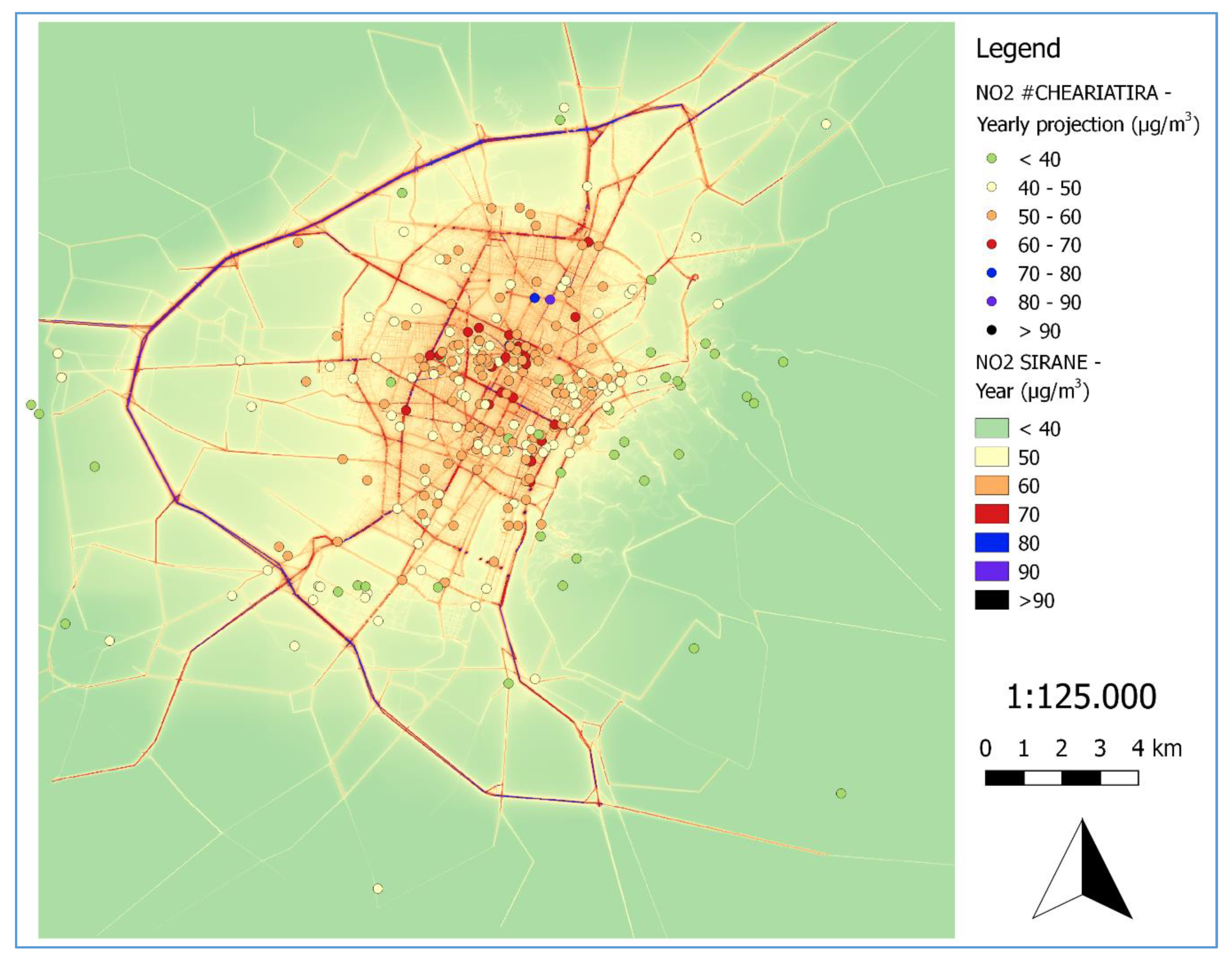
The #CHEARIATIRA citizen science campaign was developed in February 2019 in Torino (western part of the Po Valley megacity region). The aim of the campaign was public engagement with measuring NO2 concentrations in an urban area that often exceeds air quality standards. NO2 diffusion tubes were employed by citizens under our supervision. In this paper, we present the main outcomes of a combined approach between the #CHEARIATIRA campaign and the urban dispersion model SIRANE. The results were validated against the available public Air Quality Monitoring Stations (AQMS). The citizens’ passive samplers and the modelled data show a good response in central districts both during the campaign interval and by annual projection. Traffic hotspots and sensitive receptors (schools, hospital) have high concentrations of NO2. Most of the study area (83% of the tubes) is subject to an increased risk of premature death according to epidemiological literature.
Keywords:
air quality; air pollution; citizen science; diffusion tubes; NO2; SIRANE; urban dispersion model 1. Introduction
Air pollution causes chronic illness, psychological distress and economic loss, especially in densely populated areas [1,2]. In Europe, the poor air quality (AQ) is responsible of around 400,000 premature deaths every year [3]. Italy is the European country with the highest amount of life losses related to the exposures to airborne particulate matter (PM10, PM2.5), nitrogen dioxide (NO2) and ozone (O3) [4].
The Po Valley megacity, located in the north of Italy, is a hotspot for chronic air pollution [5,6]. In the last decades, the concentrations of some air pollutants like carbon monoxide (CO), metals (As, Cd, Ni, Pb) and sulphur dioxide (SO2) decreased in many urban areas (Turin and Milan above all) [7,8]; however, some AQ legislated limits—i.e., daily PM10, annual NO2, 8 h objective for O3 (the maximum daily eight-hour mean of 120 μg/m3 should not be exceeded for more than 25 days over three years)—are regularly exceeded at public air quality monitoring stations (AQMS). This scenario results from the combination of high anthropogenic emissions (traffic, domestic heating, industrial, agricultural) and unfavourable air circulation leading to stagnation and secondary pollutants’ formation [9,10,11].
The low AQ is the result of, and acts in combination with, other environmental degradation mechanisms. For example, anthropogenic sources of air pollutants are also responsible for greenhouse gases emissions. At the same time, both short-term and long-term air pollution can be exacerbated by growing wildfires events [12,13], the transformation of natural emissions and atmospheric chemistry [14] due to climate change.
In addressing this complex scenario, the engagement of communities and individuals in scientific research is pivotal. This process, called citizen science (CS), is based on the voluntary participation of nonprofessional contributors to studies, assisted by scientists during design, implementation and data analysis.
Several AQ community-driven CS projects are reported in the literature [15,16]. For example, citizens of Imperial county (California, CA, USA) promoted a “community-based air network” to expand the data from the existing public monitoring system (five samplers for 175,000 individuals on a surface of around 10,000 km2) [17]. This study employed—like many recent CS projects [18,19]—low-cost instruments. In 2019, citizens’ sensor data and machine learning were combined to map the urban air quality (UAQ) of Seoul (South Korea) [20]. Besides, CS methods were used to assess the AQ of informal settlements in Nairobi (Kenya) [21] or the effect on PM concentration from fireworks during a celebration in Medellin (Colombia) [22]. The overall positive impact of CS on the economic, social and health well-being of the target community is also reported [23,24]. Therefore, CS can lead to the mobilisation of cultural, social, economic, legal, administrative and political actors to resolve local issues.
Nitrogen oxides (NO2 and NO also referred as NOX) are formed during combustions by oxidation of nitrogen in air. The main sources of NOX both at regional and urban level are road traffic (Piemonte: 56%; Torino: 60%), industrial processes (Piemonte: 21%; Torino: 19%) and domestic heating (Piemonte: 9%; Torino: 8%) [25]. NOX cause health impairments such as respiratory morbidity and mortality, lung cancer, pneumonia, stroke and cardiovascular diseases. Data emerging from monitoring activities, baseline health information and epidemiological studies have highlighted the synergic impact of NOX, PM and O3 [26]. Besides, NOX are responsible for the formation of secondary PM and tropospheric O3. Specifically, NO2 is a good proxy of UAQ thanks to the significant difference between background values and urban concentrations [27]. Thus, NO2 concentration–response functions should be included in cost–benefit analysis for air quality policies and pollution reduction strategies, in order to provide the most effective benefits to health, environment and economy [26,28].
In this paper, we present a combined approach developed in 2019 between an urban dispersion model (SIRANE) and a citizen science campaign (#CHEARIATIRA) for the assessment of NO2 concentrations in the urban agglomeration of Torino (Piemonte region, western part of Po valley). This area comprises 25 municipalities with 1.4 million inhabitants (4th in Italy) spread over 630 km2. The domain had already been the subject of a SIRANE case study focused on 2014 [29]. Indeed, a scientific purpose of this new research was the collection of additional fine-grained atmospheric concentration data in one of the most polluted months of the year (i.e., February). The use of NO2 passive samplers (i.e., diffusion tubes) assured an easy deployment by non-experts and the recording of reliable point data, as reported in the literature [30,31,32,33]. This data was compared to the outcomes of SIRANE and validated against the available reference measurements from AQMS in Torino.
2. Materials and Methods
2.1. #CHEARIATIRA Campaign
Torino Respira (Torino Breathes) is a citizens’ committee promoting the improvement of AQ in the city of Torino and its metropolitan area. The committee supports the dissemination of scientific information on AQ as an awareness raising tool, by involving citizens, organising meetings with experts and lobbying the institutions to adopt measures to reduce air pollution. In 2019, Torino Respira launched the monitoring campaign #CHEARIATIRA. This initiative involved the citizens of Torino and a few neighbouring municipalities in the measurement of outdoor NO2 concentrations in about 300 points.
Similar to the Imperial county case study [17], the #CHEARIATIRA campaign aimed to collect NO2 concentrations data in the proximity of residences, workplaces and leisure areas in addition to those collected by the local AQMS. The latter, handled by the Regional Agency for Environmental Protection (ARPA Piemonte) from the late 1990s, verifies the compliance with legislated values in five sites within the city borders of Torino (population: 885,000 approx.).
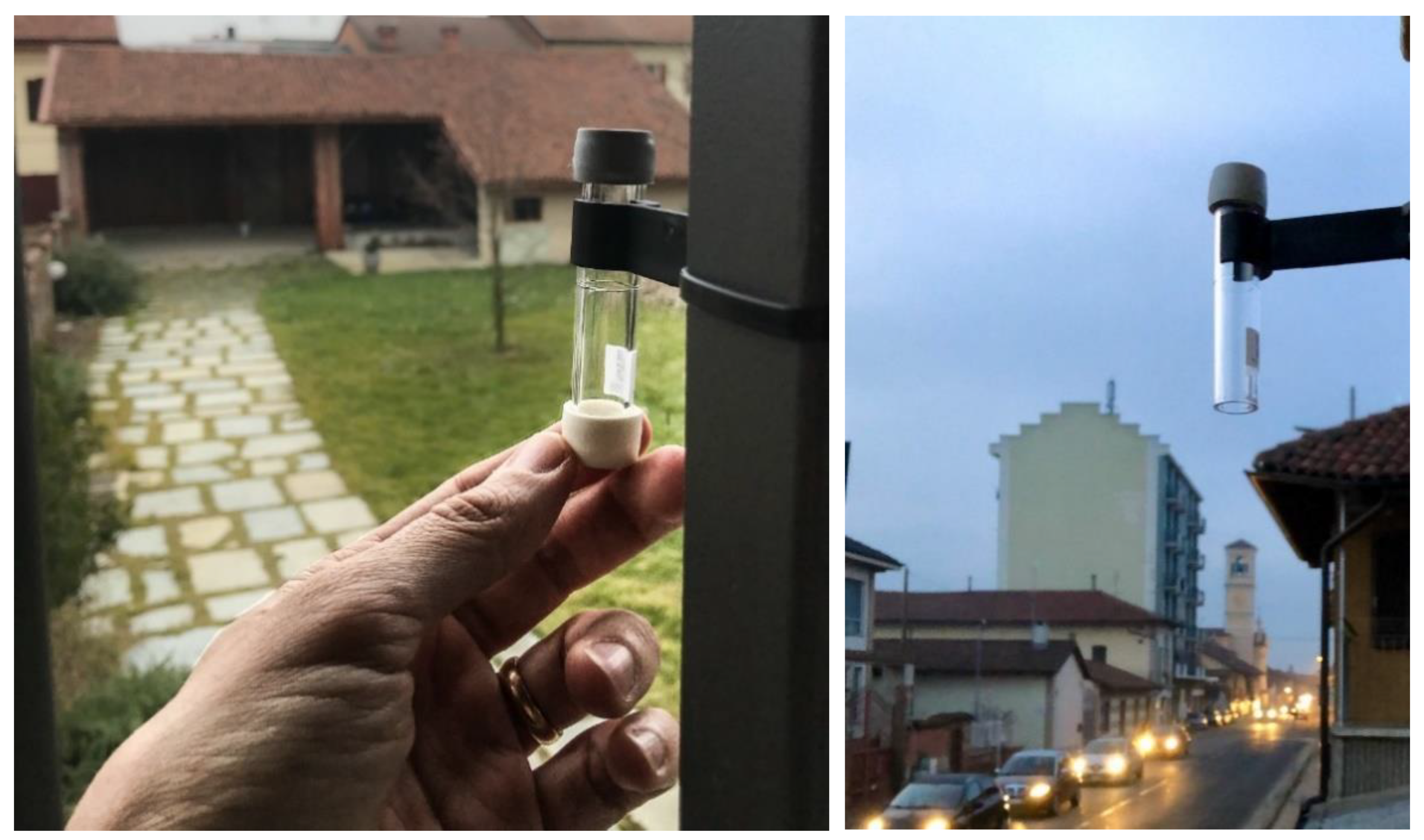
The #CHEARIATIRA campaign was developed using diffusion (Palmes) tubes. This tool, designed for the passive monitoring of gaseous NO2 in ambient air, consists of an acrylic cylinder (71.0 × 12.0 mm) fitted with grey and white thermoplastic rubber caps. Underneath the grey cap, a mesh containing a 20% Triethanolamine (TEA)/water solution chemically absorbs NO2 from the time the white cap is removed to the time it is placed back (Figure 1). The resulting nitrite ions are quantified by a UV/Visible Spectrophotometry referred to a calibration curve corresponding to standard nitrite solutions [34]. Data quality requirements and test methods for handling, installation and analysis of NO2 passive samplers were compliant with EN 13,528 norm (parts 1–3) [35,36,37]. Therefore, passive samplers approach furnished only one value for the measured interval but with a good response with reference methods [38]. On the contrary, low-cost chemical sensors could assess NO2 variations over time but presents lower performance and duration [39,40].

Figure 1.
Passive sampler during installation (left) and operational (right) phases.
The participating citizens were directly involved in purchasing and installing the tubes. The kit provided by Torino Respira included the tube, a support bracket, plastic ties and instructions. The citizens had to install and uninstall the tube in a specific interval of a 30-day duration in the month of February 2019 (recommended days: 1 February and 1 March, respectively). The exact starting and ending dates were reported by citizens on the kit’s envelope. The tubes had to be exposed: outdoors; at a height of not less than 2 m and not more than 7 m (2nd floor approx.); in open area; possibly facing a street (suggested positions: road signs, lighting poles, balconies and window grilles). The address of measurement location—chosen among private homes, schools, workplaces and other public places—was indicated by the citizens on the corresponding envelope. Thus, the envelopes were collected by Torino Respira, which sent them to a third-party accredited laboratory for analysis. Different exposure durations were used by the lab in the ambient air concentration calculation.
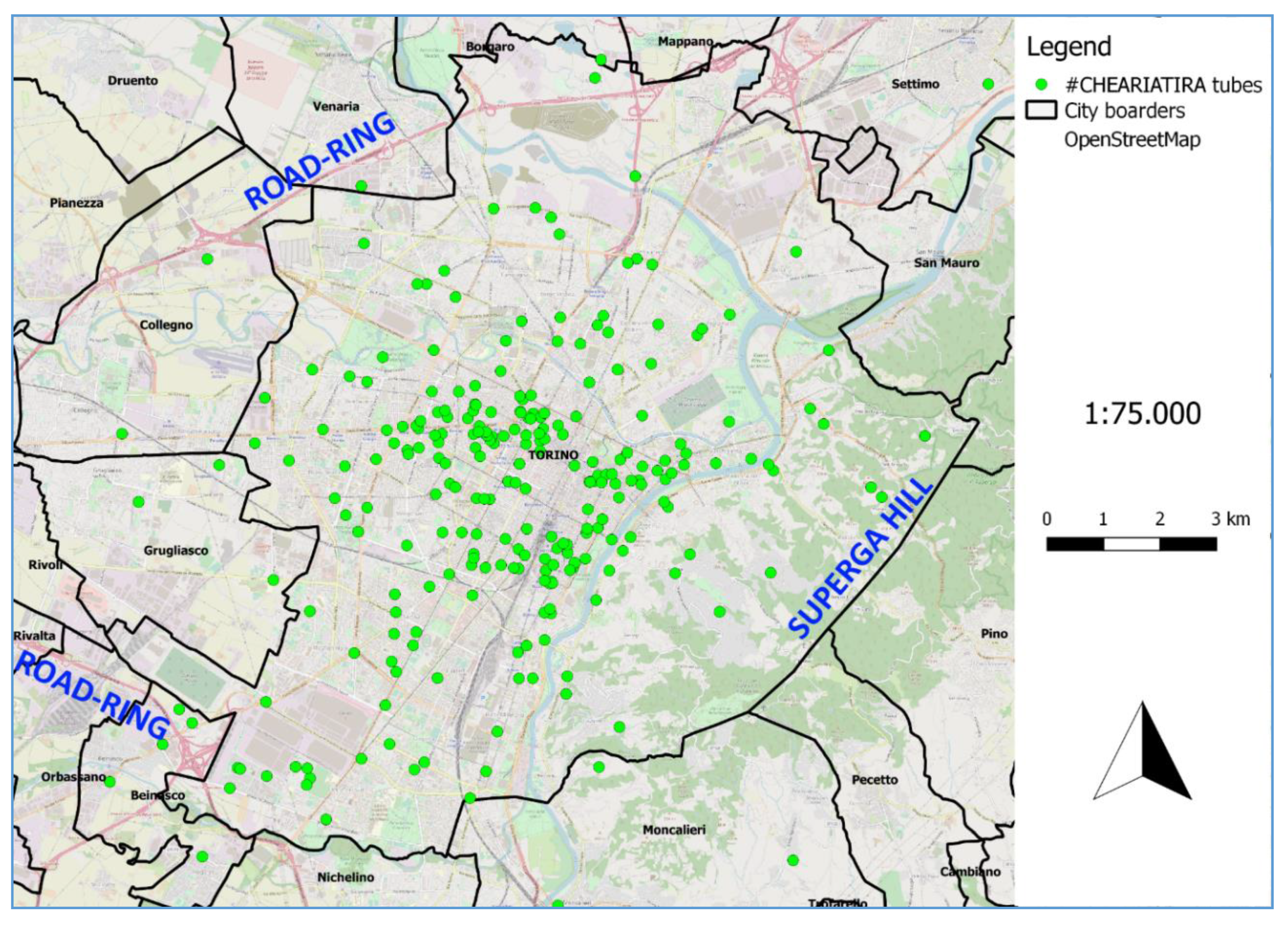
An amount of 300 tubes was installed in the Campaign (Figure 2). The study covered the wide urban agglomeration of Torino surrounded on three sides by the road-ring and, eastward, the Superga hill. Three samples have operated as blank in order to verify the reliability of the laboratory tests. Besides, four tubes were installed in the immediate vicinity (less than 10 m) to the public AQMS of Beinasco—TRM (BEI, suburban background), Torino—Consolata (CON, urban traffic), Torino—Rebaudengo (REB, urban traffic), Torino—Rubino (RUB, urban background), for direct comparison with official data (Figure 3). In fact, the accuracy of passive tubes was verified comparing the results of the ones installed at the AQMS with the monthly-averages of reference analysers at the same locations. Additional tubes, compared to those initially planned, were located close to sensitive receptors (eight schools, the Molinette hospital) and in the districts with no citizens’ tubes. The data collected and used in this paper were disseminated to the public in several events and through traditional and social media.
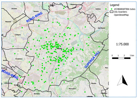
Figure 2.
Map of the distribution of tubes with city boarders (elaboration by means of QGIS 2.18).
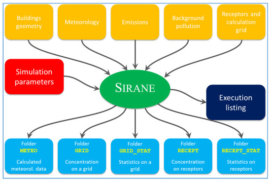
Figure 3.
Graphical workflow of SIRANE.
Meteorological patterns during the campaign, considering temperature (T), relative humidity (RH), pressure (p), wind speed (WS) and precipitation (P), are reported (Section 3.1). This data derived from the public reports of the “Stazione Meteorologica di Fisica dell’Atmosfera” (University of Torino, UniTo) [41] and the hourly data measured by the authors in the main campus of Politecnico di Torino (DIATI department).
2.2. SIRANE Modelling
The SIRANE model simulates pollutant dispersion within and above the urban canopy scale and provides hourly averaged pollutants concentrations within each street. It is based on a street network approach integrated with a Gaussian plume model for external atmosphere (above the canopy). Point, linear and surface emission sources are handled independently. The model includes also a dedicated meteorological preprocessor, a photochemical module for NOX/O3 reactions and dry/wet deposition units [42]. Over the last two decades, SIRANE has been validated both in wind tunnel [43] and in real case studies [42,44,45,46,47]. Thus, this model grants a robust correlation with measured values in urban domains if its input data are carefully parametrised (especially for traffic emissions) [44,48]. A graphical workflow of the model is reported (Figure 3).
A first application of the model in the city of Torino focussing to the year 2014 was recently achieved [29]. Starting from such case study, a new scenario for the year 2019 was advanced during this research. The traffic emissions were estimated on a network of 12,148 streets by a bottom-up approach based on: the vehicle fleet database of the Metropolitan area of Torino released by the Automobile Club d’Italia (ACI); the fluxes from the local traffic agency (5T s.r.l.); the emission factors computed by the Istituto Superiore per la Protezione e la Ricerca Ambientale (ISPRA) using the COPERT model (v.5.2.2). The latter is the reference European standard model to estimate traffic emissions by vehicle typology, EURO standard, fuel and engine size; it accounts both exhaust and non-exhaust emissions in urban, rural and highway settings [49]. Thus, ISPRA’s inventory—submitted every year to the European Environment Agency (EEA)—is the Italian reference to attest the compliance of national emissions with EU commitments to protect the population from air pollution.
Starting from 1992, the available ISPRA database (1990–2018) shows a decreasing trend of traffic-related NOX emissions on a national base [50]. The reduction between 2014 to 2018 was 19%. Focussing to the Metropolitan area of Torino, the overall emission factor decreased by 31% in the same interval. Despite an increase of the total vehicles fleet (+3.3%), this trend is most likely due to the replacement of vehicles with others with lower emission factors (recent EURO classes, hybrids). Considering the same traffic fluxes of the 2014’s study [29] (further updated data was not available), the emissions on the street network were updated using the most recent ISPRA’s emission factors (2019) and local COPERT-based vehicle fleet (2018).
The other contributions to emissions were estimated starting from the last release (2013) of the Inventory of Regional Emissions in Atmosphere (IREA) [25]. Unfortunately, this public data is quite dated and available only with the spatial resolution of the whole city. Thus, the total domestic heating emissions of Torino were disaggregated using buildings data and considering the coverage of the existing district heating network (TLR). This data was then adjusted by −20% following the trend of domestic heating emissions for the whole Piemonte region determined by ISPRA [51]. The main industrial plants, the incinerator (TRM) and urban tunnels were handled as point emissions like in 2014′s case study. Residual emissions were homogeneously distributed in the city. Furthermore, the inputs corresponding to the background pollution (from suburban areas) and to the meteorological factors were updated to the year 2019.
According to the literature [44,52], the model results were validated against measured data at AQMS using the following performance criteria: Fractional Bias (−0.3 ≤ FB ≤ 0.3), Relative Error (ER), square root of the Normal Mean Square Error (√NMSE ≤ 2), Correlation Coefficient (R), Mean Geometrical Bias (0.7 ≤ MG ≤ 1.3), Geometrical mean squared variance (VG ≤ 1.6); Fraction in a Factor of two (0.5 ≤ FAC2 ≤ 2).
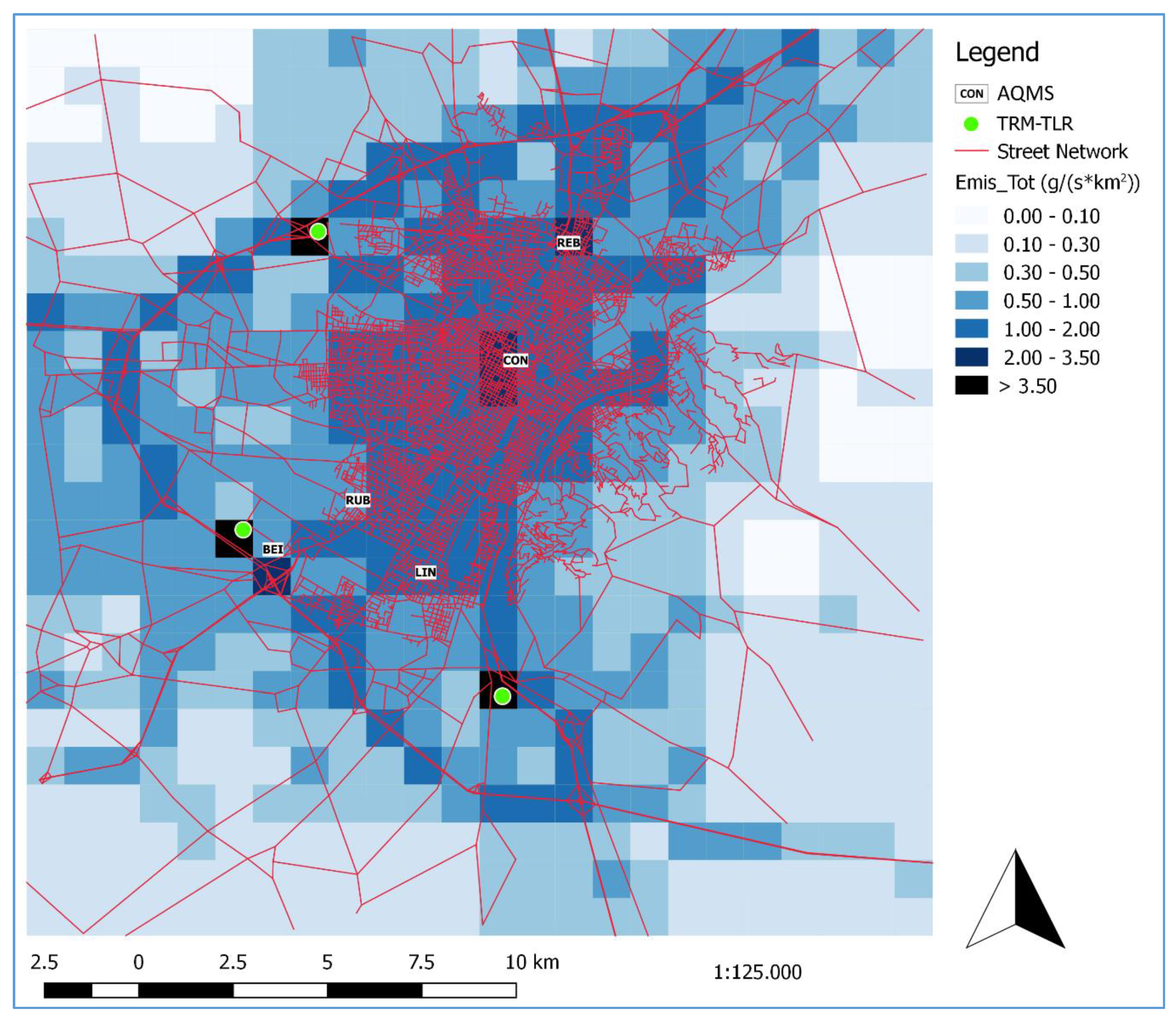
Then, the #CHEARIATIRA locations (receptors) were located on the computational grid using the addresses declared on envelopes. When available, any additional information indicated on the envelopes (front of street, courtyard, floor) was used to manually adjust their position on the map. The modelled and measured data at receptors were then compared. A summary of the AQMS and TRM/TLR plants locations, the street network and the total estimated average annual emissions of NOX normalised per square kilometre (g/(s × km2)) is illustrated in Figure 4.
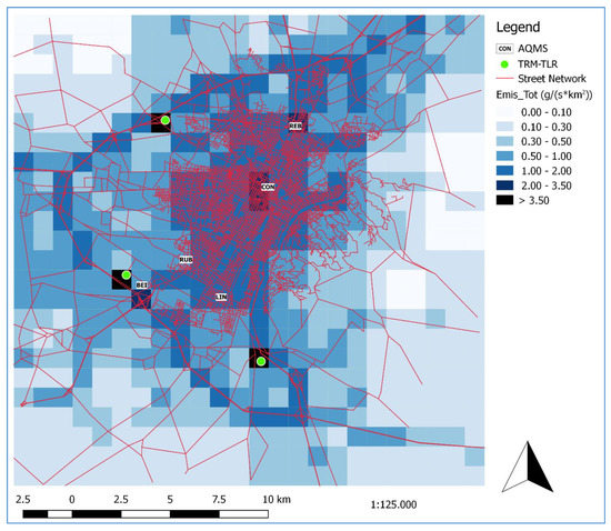
Figure 4.
Map of the simulation domain with AQMS locations, TRM and TLR plants, street network and total annual NOX emissions normalised per square kilometre (g/(s × km2)) (elaboration by means of QGIS 2.18).
3. Validation
3.1. #CHEARIATIRA Campaign
Of the 300 kits initially distributed, 277 were recovered. One of the four tubes installed at the AQMS was stolen (Torino-Rubino). Excluding the three blank tubes, subtracted from the real samples, the data size is n = 274.
From the analysis of envelopes information, the main target environments chosen by citizens were the outdoors of private homes (233, 84%). Part of them (78, 26%) were installed close to main arteria and urban squares, including road intersections. Three tubes (~1%) were located in public parks. Hence, only two tubes (~1%) were explicitly declared “in courtyard” on envelopes.
Most of the tubes were installed (85%) and uninstalled (80%) within 1st of February and 1st of March (± 1 day). The concentrations were analysed, considering the exposure time of each tube and did not need further correction. Thus, the samplers that did not respect such dates have only a residual error that depends on the higher concentrations of the last days of January (for the tubes installed too early) or the lower values that occurred in the first week of March (for tubes uninstalled too late).
The descriptive statistics of NO2 concentrations for the #CHEARIATIRA dataset, the NO2 monthly-averages of AQMS stations and the main meteorological indicators (T, RH, WS) are summarised in Table 1. In addition to the four selected sites where tubes were installed, the AQMS monthly averages included the data from Torino-Lingotto station (LIN, urban background, Figure 4). Rainy days were recorded only at the beginning of the Campaign (1−3 February, total cumulated rain =22.4 mm).

Table 1.
Summary of NO2 concentrations of #CHEARIATIRA samples, NO2 monthly-averages of AQMS and daily meteorological dataset for the Campaign period (1st February and 1st March).
In Table 1, both the raw NO2 concentrations from the laboratory tests (_raw) and the results adjusted after the accuracy analysis (_adj) are reported. The latter, returned an underestimation of NO2 concentrations of 13% by the three passive tubes compared to corresponding AQMS reference analysers. In order to obtain a more robust accuracy verification, the data in Torino have been coupled with 11 other analogous tubes located in the proximity of public stations during similar CS campaigns carried out in Milano, Brescia and Roma [53]. On average, the passive samplers underestimate the NO2 concentrations by 11%.
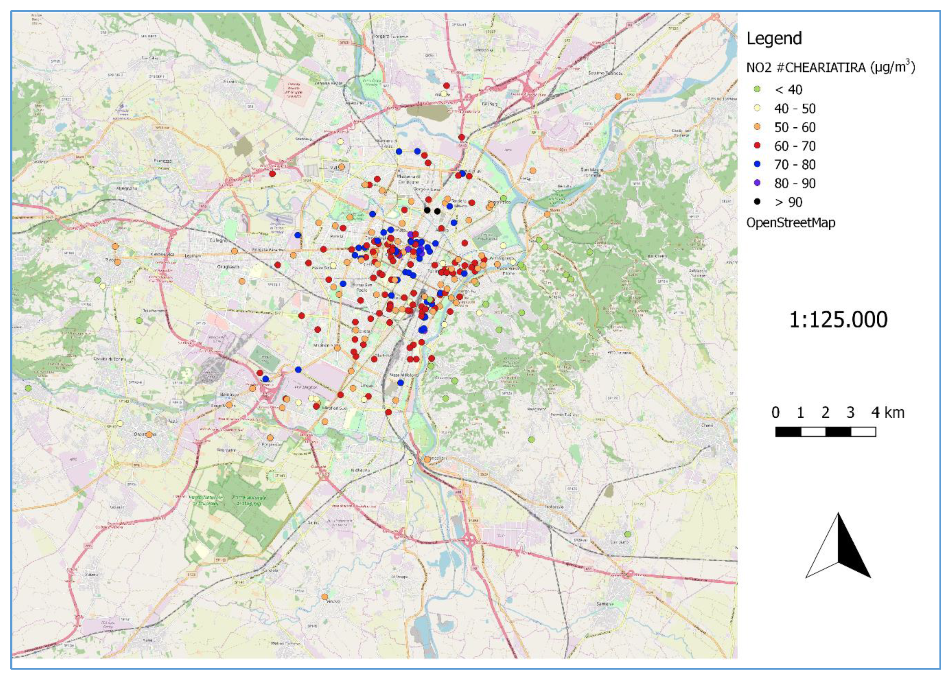
The spatial distribution of sampled data (Figure 5) displays some traffic hotspots at the roundabout of Piazza Baldissera and close to heavily trafficked arteria (Corso Dante, Corso Inghilterra, Corso Regina Margherita, Via Principe Oddone). High concentrations in the areas of Barriera di Milano, Cit Turin and San Donato were recorded. The lowest levels correspond to the tubes located in the hill of Torino (Tetti Bertoglio, Via Mongreno, Via Lavazza). All the nine sensitive receptors (Table 2) have values above 40 μg/m3; one of them (Liceo Alfieri) falls within the ten highest values of the Campaign. The tube located in the Molinette hospital has a concentration of 67.9 μg/m3 despite it was installed on a balcony in the 2nd floor facing on an internal courtyard (not directly exposed to road traffic).
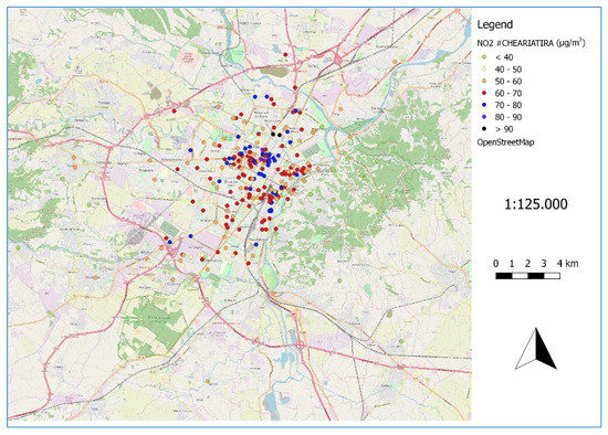
Figure 5.
Map of NO2 concentrations referred to #CHEARIATIRA samples for the campaign period (elaboration by means of QGIS 2.18).

Table 2.
NO2 concentrations at the sensitive receptors for the campaign period.
Then, the previous observations were aggregated considering the eight subadministrative areas of Torino (called “Circoscrizioni”, Figure 6). The ones with the worse data embrace the central districts of the city (C1, C3, C4, C5). An exception is represented by C7, which has high values in the district of Aurora and very low values in Sassi and Madonna del Pilone. The highest amount of tubes was installed in C1 (57) while only 12 and 15 installations in C5 and C6 are reported, respectively. No correlation between average concentration and amount of installed tubes is observed (R2 = 0.08).
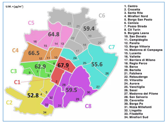
Figure 6.
Map of NO2 concentrations by “Circoscrizioni” for the campaign period.
Furthermore, the C1 is partitioned in a restricted traffic area (ZTL) and in an un-restricted traffic area (no-ZTL). A slight variability between this two subsections can be observed (average values: ZTL = 66.7 μg/m3; no-ZTL = 68.9 μg/m3).
3.2. SIRANE Modelling
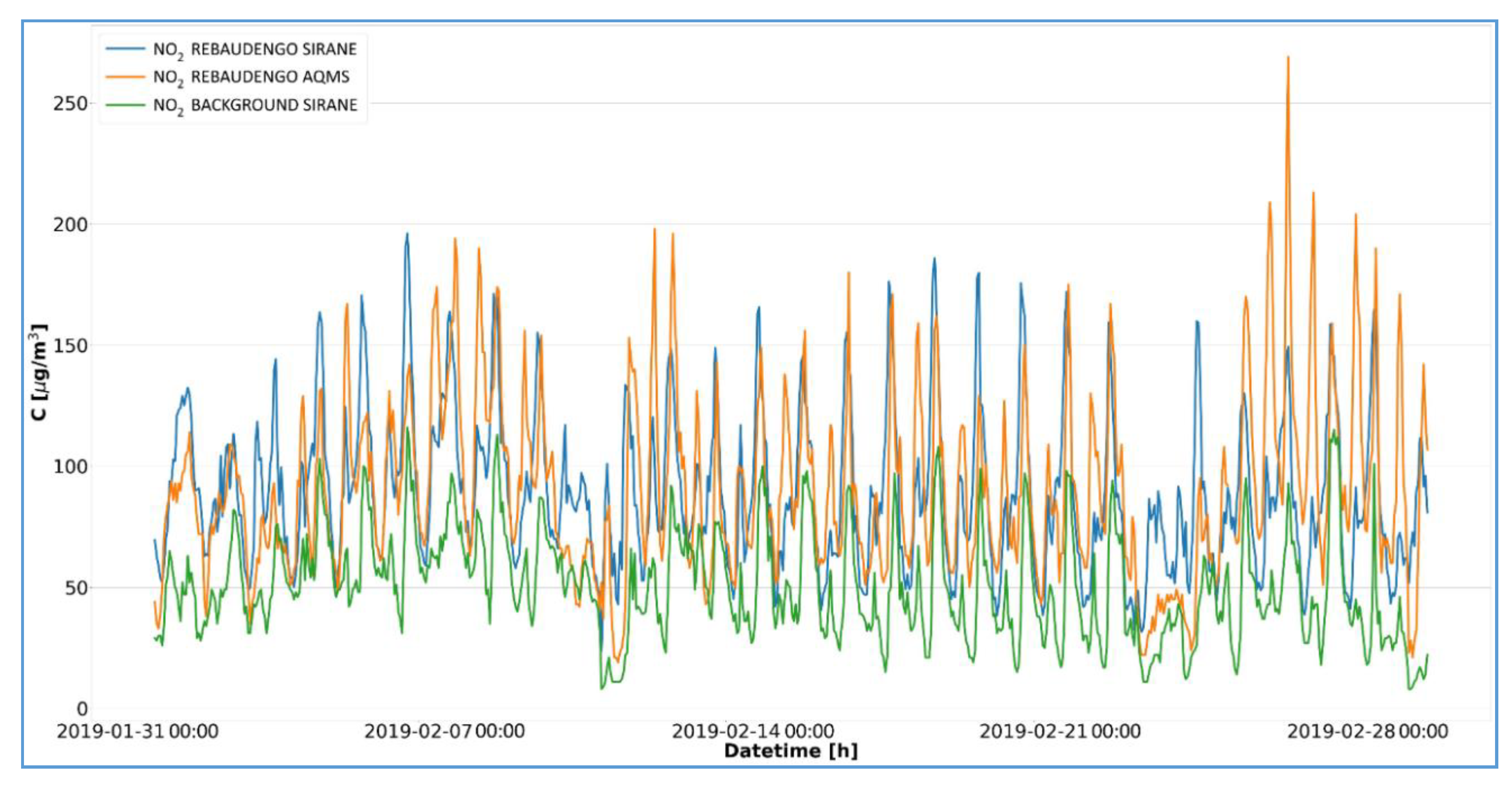
The outcomes of SIRANE substantially agree with public measurements (Table 3). By average, the modelled (71.9 ± 11.2 μg/m3) and measured (70.1 ± 16.4 μg/m3) data accord at the five receptors. Also, the performance criteria are entirely respected for all the receptors. The FB, √NMSE, MG, VG and FAC2 falls within their validation intervals and NO2 values are associated with a low relative error (ER = 0.24–0.34). Conversely, a moderate correlation (R = 0.57–0.67) is observed. This result depends on the variance between the hourly modulation of emissions and the real (day-by-day) patterns of pollutants releases. For example, in some traffic stations (Consolata, Rebaudengo), some of high daily peaks are intrinsically underestimated by the model (like the maximum of 269 μg/m3 recorded the 26 February 2019 in Rebaudengo, which represents the 4th highest value of the decade). The station of Lingotto has the worst performances and presents a substantial average overestimation of NO2 concentrations. Conversely, Rebaudengo has the best computational results among the five sites. In Figure 7 the time-series of this station—showing SIRANE modelled (blue) and AQMS measured (orange) NO2 concentrations—is reported. Compared to the background values used for SIRANE (green), the contribution of local emissions sources within the city boarders is evident. The results fit with the previous applications of SIRANE [44,46] and, therefore, confirm the consistency of the SIRANE case study.

Table 3.
Comparison of mean, max and median concentration and performance parameters of SIRANE against AQMS monitored values.
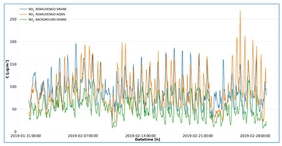
Figure 7.
Time plot of NO2 concentrations at Rebaudengo (elaboration by means of Python 3.6.5).
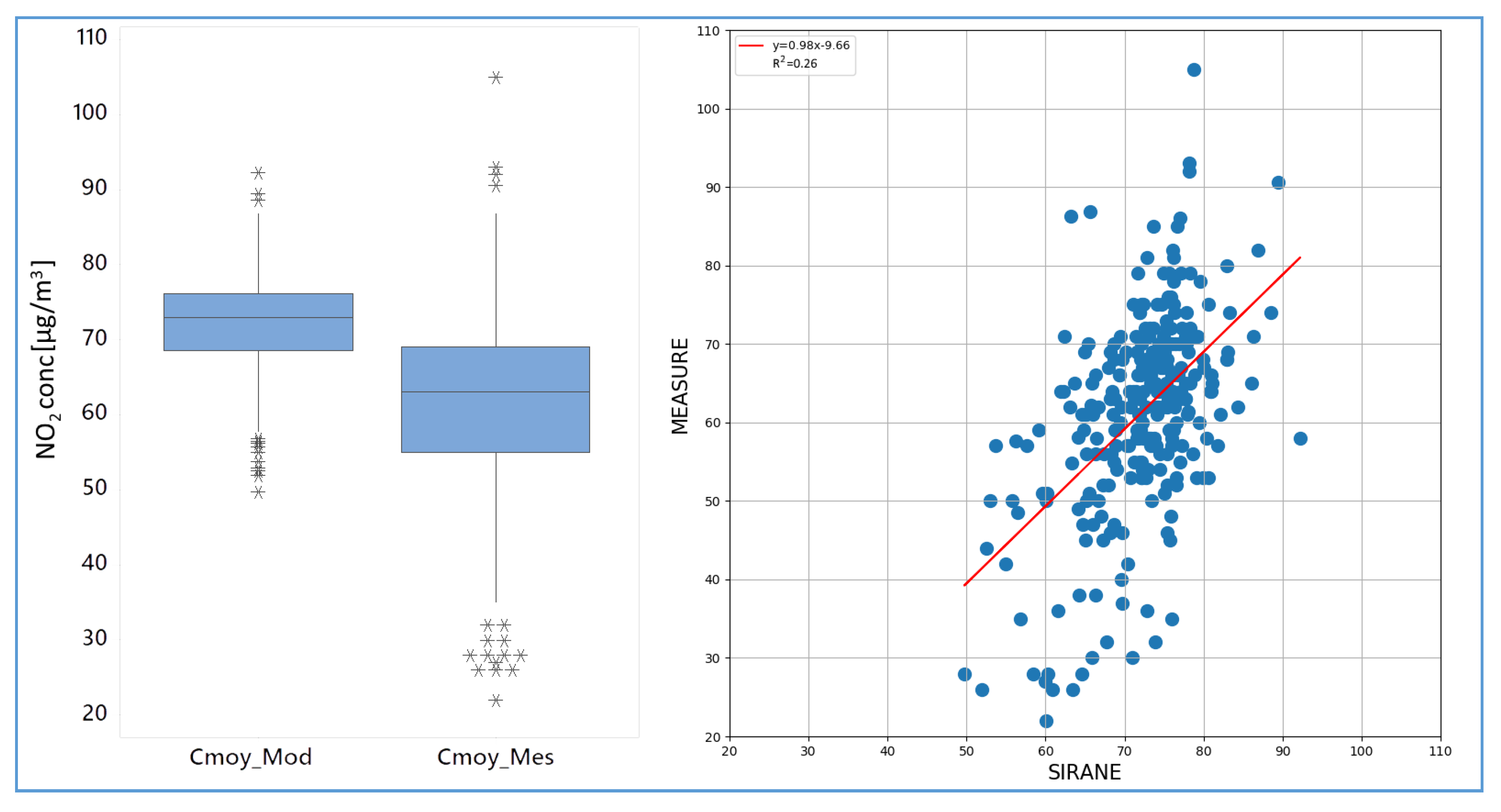
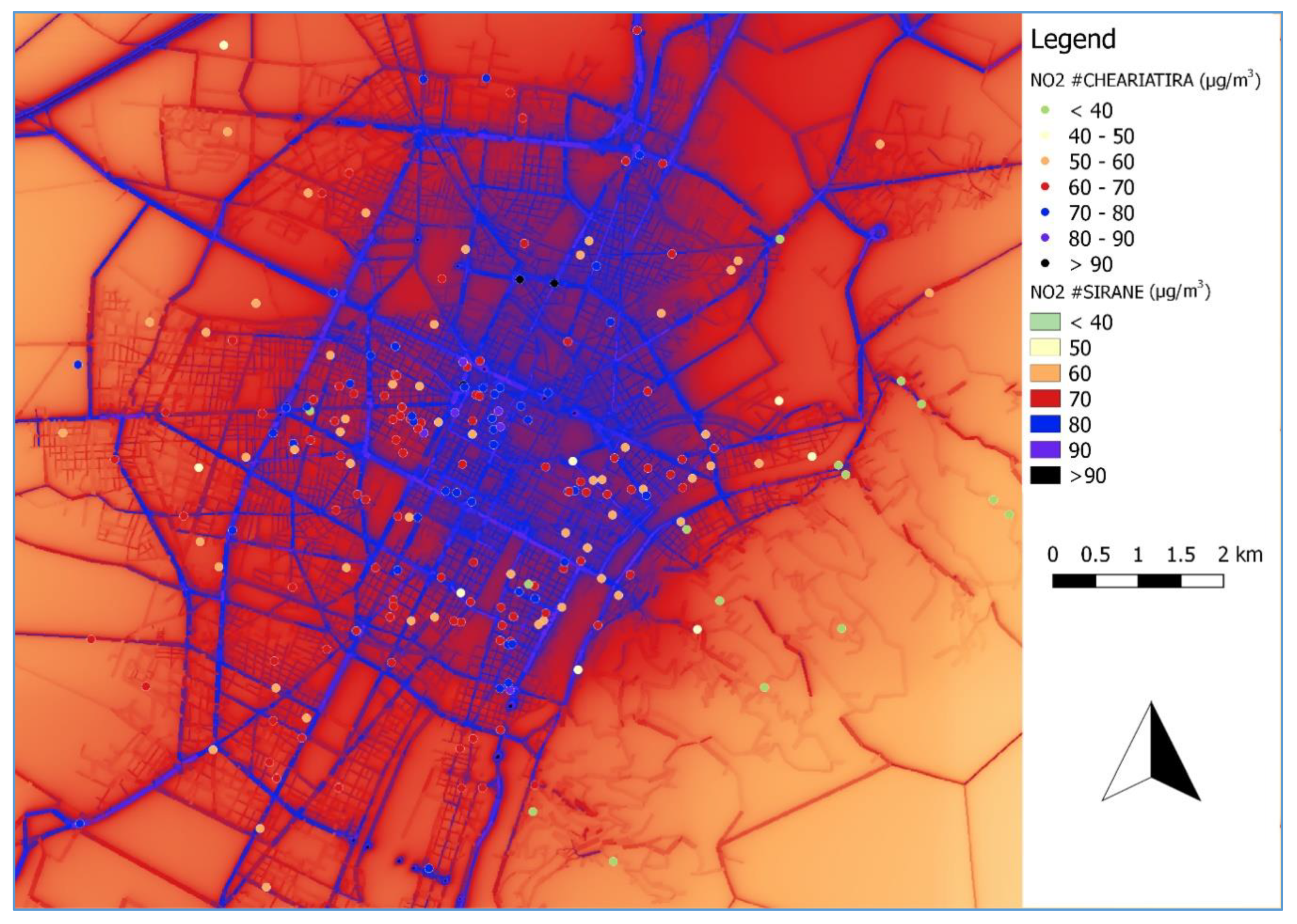
Then, #CHEARIATIRA samples were compared to SIRANE outputs. The passive tubes located at the AQMS show lower averaged NO2 concentrations (71.5 ± 5.8 μg/m3) compared to both model (76.8 ± 12.7 μg/m3) and public measurements (77.9 ± 17.3 μg/m3). Therefore, an analysis of variance (ANOVA) was developed to check whether the means of the tubes’ and the model’s datasets at the receptors were statistically equal or not (n = 274, α = 0.05). We found a p-value below the significance level (1.05−31 < α), so we can affirm that, by average, the dataset of samples is statistically lower compared to the corresponding modelling results. These fallouts occur despite the previous accuracy correction of samples (Section 2.1). An elevated linear response (m = 0.98) is observed but this outcome is driven by a negative zero-offset (q = −9.66 μg/m3). Besides, the coefficient of determination (R2 = 0.26) confirms that the two dataset are dispersed (Figure 8). The greatest differences occur for low concentrations of NO2 and few very high values measured with respect to model. The map of tubes concentrations against modelled data (Figure 9) shows that the agreement between the two datasets is the highest in areas closest to roads and decreases moving far from the street network. Moreover, the best correspondence is located in the central districts and the worst in peripheral areas.
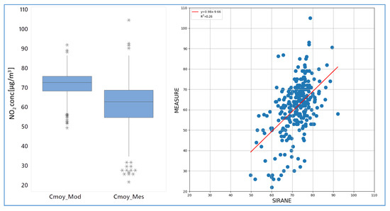
Figure 8.
Statistical distribution of average NO2 concentrations modelled by SIRANE (_Mod) and measured by tubes (_Mes) at receptors using boxplot (left) and scatterplot (right) for the campaign period (elaboration by means of MiniTab® 17.1.0 and Python 3.6.5).

Figure 9.
Map of average NO2 concentrations modelled by SIRANE with #CHEARIATIRA samples for the campaign period (elaboration by means of QGIS 2.18).
4. Exposure Assessment
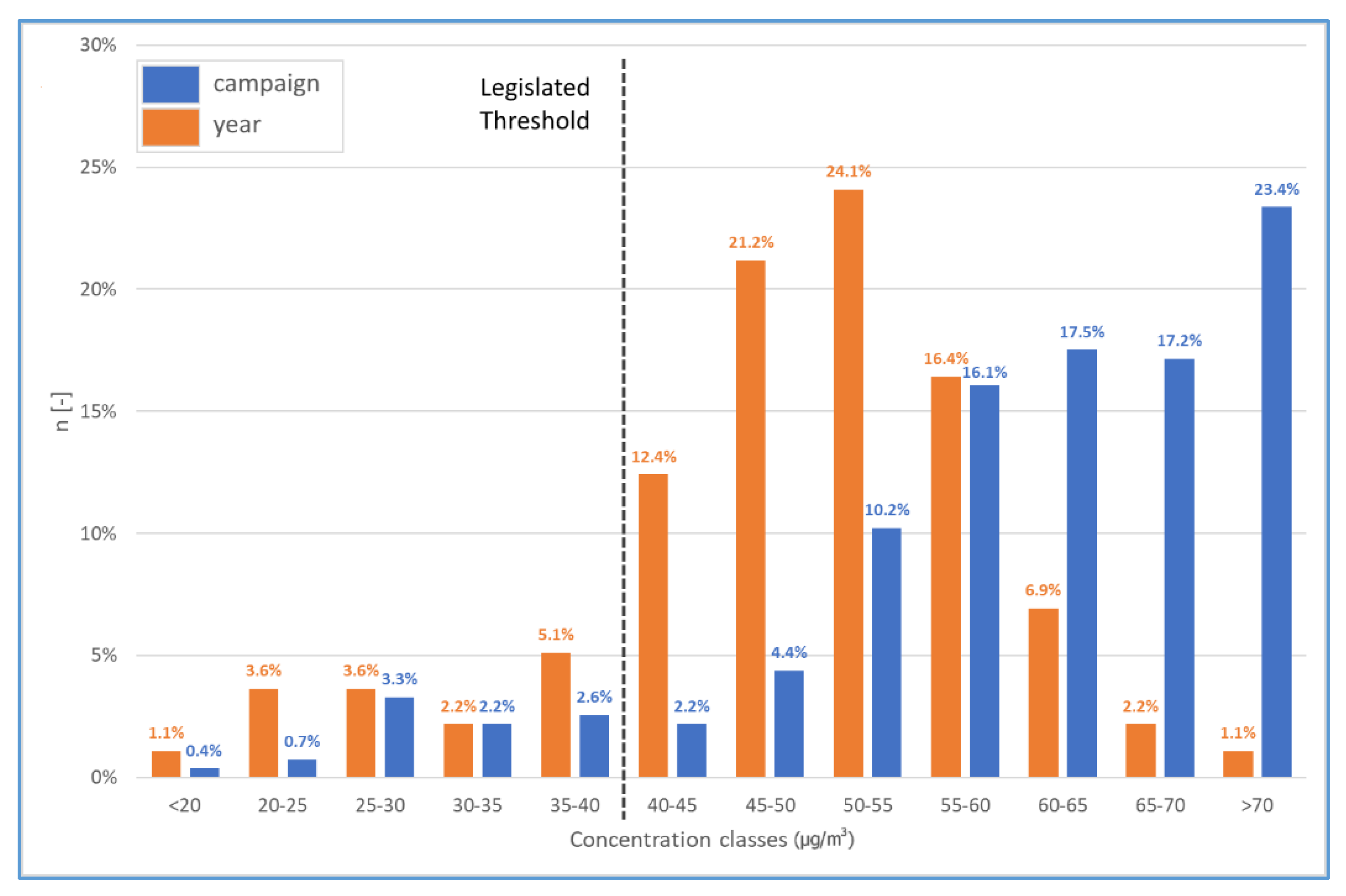
The assessment of population exposure refers to the legislated values. Indeed, in order to correlate the data with the mean annual NO2 limit, the results of the Campaign were projected on a yearly time scale using the average ratio between NO2 concentrations recorded in February and the corresponding annual values. The calculation was made on the last four years using the five ARPA datasets. The resulting ratio is 0.80 ± 0.05. This value, multiplied by the campaign records, foresees the corresponding yearly concentrations (orange, Figure 10).
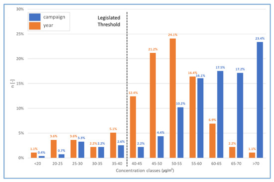
Figure 10.
Distribution of #CHEARIATIRA samples for the campaign period (blue) and annual projection (orange).
An annual decrease compared to the data recorded in February (blue, Figure 10) was observed. However, 84% of the samples still exceeded the 40 μg/m3 threshold. The majority of extrapolated data ranged between 45 μg/m3 and 55 μg/m3. Similar values were observed in the CS campaign of Milano (84%), but not in Roma (60%) and Brescia (10%) [53].
These results are confirmed by the values computed by the model for the whole 2019 (Figure 11). As expected, the yearly NO2 concentrations are significantly lower than in February. The results accord to the reduction of emissions (domestic heating) and the improvement of pollutants dispersion conditions of the warm season.
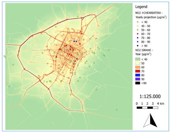
Figure 11.
Map of average NO2 concentrations modelled by SIRANE for 2019 with #CHEARIATIRA annual projection (elaboration by means of QGIS 2.18).
The outcomes of different epidemiological studies, coupled with the results of the research, let us foresee which areas of the city are at higher health risk for population exposure to NO2. The EpiAir epidemiological study, targeted to Torino and other nine Italian cities [54], found statistically significant associations between the increase by 10 μg/m3 of NO2 concentration and mortality (natural +2.09%; cardiac +2.63%; respiratory +3.48%). The authors affirm that “these associations were independent from those of PM10 and O3” and, thus, should be accounted entirely for NO2. In addition, the HRAPIE project by WHO [26] affirms that each 10 μg/m3 increase in NO2 concentrations (from 20 μg/m3) corresponds to an increased risk of premature death of 5.5% for adults aged above 30 years old. The authors state that this result accounts the additive effect of NO2 to the overall air pollution.
Therefore, we assessed the NO2 concentration—health response functions assuming no effects below 40 μg/m3 as cautionary consideration from the two previous research studies. The same assumption was made by Piemonte region in its Air Quality Regional plan, which accounted for more than 3000 years of life lost in 2015 on the whole city [55]. The results (Figure 12) show that most of annually projected concentrations recorded by passive tubes (83%) corresponded to an increased risk of premature death between 5.5% and 16.5%.
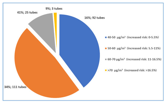
Figure 12.
Pie chart of increased risk of premature death corresponding to sampled values.
5. Discussion
The #CHEARIATIRA campaign achieved significant participation from citizens. The distribution of diffusion tubes covered the entire city. The results are in line with the accuracy recorded in other CS campaigns in Italy and with AQMS records for the period.
On a monthly basis, after accuracy correction, 91% of samples exceeded the annual legislated threshold (40 μg/m3), despite direct correlation between annual limits and monthly averages should be avoided. Indeed, 84% and 23% of tubes exceed the value of 50 μg/m3 and the AQMS average (70.4 μg/m3), respectively. The tubes with the highest concentrations were located close to the main urban arteria. Some of the tubes with more concern were close to sensitive receptors. All schools exceed the legislated threshold.
The aggregated analysis of “Circoscrizioni” shows, as predicted, that those with the highest average concentrations (above 60 μg/m3) have also the greatest population density of the city (C1, C4, C5, C3). Furthermore, these areas correspond to where most tertiary activities—attracting workers also from neighbour cities—are located. Focussing on C1, the narrow difference between ZTL and no-ZTL subsections could be ascribed to a limited effect of the traffic restrictions in the ZTL area, which involves few hours per day (3 h). Considering NO2 samples, the hill of Torino shows the lowest concentrations. However, only one tube returned a concentration below 20 μg/m3 in the whole campaign.
The model shows a high performance compared to public measurements. Conversely, some differences between tubes and simulation could be observed.
A limit of #CHEARIATIRA approach is represented by the lack of accurate descriptions of the locations of the passive tubes. In fact, the model receptors were mostly settled using only their addresses (90% approximately): some of the receptors which were placed on the maps on the side of roads might have been measured in courtyards or not in open fields. Another issue is the overestimation in the tubes that were installed too early in January and the underestimation those that were uninstalled to late in March (Section 3.1). Though the lab has corrected the concentrations by their real exposure time, the error is the larger in the shift between sampling interval and assessment period.
On the side of the model, a limit is surely represented by the use of a single background dataset for the whole domain. This limitation affects the edge areas of the domain where the contribution of urban emissions is lower compared to suburban concentrations. This outcome confirms the observed deterioration of the correspondence between the tubes and the model at external receptors. Furthermore, the model lacks performance due to the terrain. We can affirm that the model overestimates the NO2 concentrations in the hill of Torino, where most of the lowest values of #CHEARIATIRA were sampled. Further secondary improvements will be made on emissions input data when more up-to-date databases will become available.
Finally, apart from such inaccuracies, the campaign and the modelling results have a good correlation. In February, both the model and the campaign showed high concentrations in sensitive receptors and the greatest compliance is achieved in the central districts. Conversely, SIRANE’s 2019 computation and the projection of #CHEARIATIRA data on an annual basis have a greater mutual response for suburban areas than in February. The latter is due to an overestimation of the background concentrations of SIRANE in wintertime.
Beyond the findings, some of the limitations of this work should be highlighted. The Campaign covered a large urban area, but the samplers were mostly installed within the municipality boarders of Torino. The dense distribution of sensors in this city ensured a good comparison with the model. However, peripheral areas of the study domain lack of resolution, which could have been greater with a spreader distribution of samplers. Another limitation is the availability of only one value, corresponding to the average conditions during the Campaign, for each receptor. Compared to other CS [17,19,21], a replication of this study in the summertime and the implementation of low-cost sensors and gas analysers at the receptors could ensure further point measurement of local pollution trends over time. Finally, in line with other research [56,57], indoor measurements should be coupled to that of the outdoors in order to assess personal exposure of population within the domain.
6. Conclusions
The #CHEARIATIRA campaign boosted the citizens’ awareness of the AQ issue in Torino. Indeed, the initiative has been renewed in 2020, with more participants (over 420 people and 700 samplers) from Torino and 29 neighbouring municipalities (Carmagnola, Carignano, Fossano and Vinovo, above all). Following the observed high concentration at sensitive receptors, passive samplers have been installed to over 90 schools thanks to the support of a local banking foundation (Compagnia di San Paolo). A further objective of this second edition is to compare the data with those of the previous data set and thus increase the scientific reliability of the results. These outcomes will be discussed in a following paper.
Author Contributions
Conceptualization, M.B., P.S., R.M. and M.C.; Data curation, M.B.; Formal analysis, M.B.; Investigation, M.B. and R.M.; Methodology, M.B.; Resources, P.S., R.M. and M.C.; Software, P.S.; Supervision, P.S., R.M. and M.C.; Validation, M.B., P.S., Federica Pognant, R.M. and M.C.; Writing—original draft, M.B.; Writing—review & editing, M.B., P.S., F.P., R.M. and M.C. All authors have read and agreed to the published version of the manuscript.
Funding
The 2019′s #CHEARIATIRA campaign was founded by private citizens. Further support for the development of this research was provided by the two scientific institutions of academic authors (Politecnico di Torino—DIATI department in the frame of climate_change@polito project (Moving lab), and Ecole Centrale de Lyon—LMFA laboratory).
Acknowledgments
We thank all the citizens and volunteers involved in the #CHEARIATIRA campaign. P.S. acknowledges the Région Auvergne Rhône Alpes Project SCUSI.
Conflicts of Interest
The authors declare no conflict of interest.
References
- Lelieveld, J.; Evans, J.S.; Fnais, M.; Giannadaki, D.; Pozzer, A. The contribution of outdoor air pollution sources to premature mortality on a global scale. Nature 2015, 525, 367–371. [Google Scholar] [CrossRef] [PubMed]
- WHO. WHO|Global Health Risks Report. Available online: http://www.who.int/healthinfo/global_burden_disease/global_health_risks/en/ (accessed on 22 May 2017).
- WHO. WHO|Ambient Air Pollution: A Global Assessment of Exposure and Burden of Disease. Available online: http://www.who.int/phe/publications/air-pollution-global-assessment/en/ (accessed on 11 May 2017).
- European Environmental Agency. EEA Air Quality in Europe—2015 Report; European Environmental Agency: Copenhagen, Denmark, 2015. [Google Scholar]
- Van Donkelaar, A.; Martin, R.V.; Brauer, M.; Kahn, R.; Levy, R.C.; Verduzco, C.; Villeneuve, P.J. Global Estimates of Ambient Fine Particulate Matter Concentrations from Satellite-Based Aerosol Optical Depth: Development and Application. Environ. Health Perspect. 2010, 118, 847–855. [Google Scholar] [CrossRef]
- ESA Copernicus Sentinel-5P: Maps of Nitrogen Dioxide Pollution. Available online: https://www.esa.int/Our_Activities/Observing_the_Earth/Copernicus/Sentinel-5P/Nitrogen_dioxide_pollution_mapped (accessed on 31 May 2019).
- Rossi, G.; Vigotti, M.A.; Zanobetti, A.; Repetto, F.; Gianelle, V.; Schwartz, J. Air Pollution and Cause-Specific Mortality in Milan, Italy, 1980–1989. Arch. Environ. Health Int. J. 1999, 54, 158–164. [Google Scholar] [CrossRef] [PubMed]
- Giulianelli, L.; Gilardoni, S.; Tarozzi, L.; Rinaldi, M.; Decesari, S.; Carbone, C.; Facchini, M.C.; Fuzzi, S. Fog occurrence and chemical composition in the Po valley over the last twenty years. Atmos. Environ. 2014, 98, 394–401. [Google Scholar] [CrossRef]
- Baklanov, A.; Kukkonen, J.; Finardi, S.; Beekmann, M.; Sokhi, R.; Mahura, A.; Ginsburg, A.; Mažeikis, A. Meteorological Conditions Favouring Development of Urban Air Pollution Episodes. Megapoli Sci. Rep. 10-10 2013, 15, EGU2013-12835. [Google Scholar]
- Bigi, A.; Ghermandi, G. Trends and variability of atmospheric PM2.5 and PM10–2.5 concentration in the Po Valley, Italy. Atmos. Chem. Phys. Discuss. 2016, 16, 15777–15788. [Google Scholar] [CrossRef]
- Diémoz, H.; Gobbi, G.P.; Magri, T.; Pession, G.; Pittavino, S.; Tombolato, I.K.F.; Campanelli, M.; Barnaba, F. Transport of Po Valley aerosol pollution to the northwestern Alps—Part 2: Long-term impact on air quality. Atmos. Chem. Phys. Discuss. 2019, 19, 10129–10160. [Google Scholar] [CrossRef]
- Bo, M.; Mercalli, L.; Pognant, F.; Berro, D.C.; Clerico, M.; Luca, M.; Federica, P.; Daniele, C.B.; Marina, C.; Matteo, B. Urban air pollution, climate change and wildfires: The case study of an extended forest fire episode in northern Italy favoured by drought and warm weather conditions. Energy Rep. 2020, 6, 781–786. [Google Scholar] [CrossRef]
- Westerling, A.L.; Bryant, B.P. Climate change and wildfire in California. Clim. Chang. 2007, 87, 231–249. [Google Scholar] [CrossRef]
- Jacob, D.J.; Winner, D.A. Effect of climate change on air quality. Atmos. Environ. 2009, 43, 51–63. [Google Scholar] [CrossRef]
- Wiggins, A.; Wilbanks, J. The Rise of Citizen Science in Health and Biomedical Research. Am. J. Bioeth. 2019, 19, 3–14. [Google Scholar] [CrossRef]
- Mahajan, S.; Kumar, P.; Pinto, J.A.; Riccetti, A.; Schaaf, K.; Camprodon, G.; Smári, V.; Passani, A.; Forino, G.; Riccetti, A. A citizen science approach for enhancing public understanding of air pollution. Sustain. Cities Soc. 2020, 52, 101800. [Google Scholar] [CrossRef]
- English, P.; Olmedo, L.; Bejarano, E.; Lugo, H.; Murillo, E.; Seto, E.; Wong, M.; King, G.; Wilkie, A.; Meltzer, D.; et al. The Imperial County Community Air Monitoring Network: A Model for Community-based Environmental Monitoring for Public Health Action. Environ. Health Perspect. 2017, 125, 074501. [Google Scholar] [CrossRef] [PubMed]
- Ford, B.; Pierce, J.R.; Wendt, E.; Long, M.; Jathar, S.H.; Mehaffy, J.; Tryner, J.; Quinn, C.W.; Van Zyl, L.; L’Orange, C.; et al. A low-cost monitor for measurement of fine particulate matter and aerosol optical depth – Part 2: Citizen-science pilot campaign in northern Colorado. Atmos. Meas. Tech. 2019, 12, 6385–6399. [Google Scholar] [CrossRef]
- Benabbas, A.; Geißelbrecht, M.; Nikol, G.M.; Mahr, L.; Nähr, D.; Steuer, S.; Wiesemann, G.; Müller, T.; Nicklas, D.; Wieland, T. Measure particulate matter by yourself: Data-quality monitoring in a citizen science project. J. Sensors Sens. Syst. 2019, 8, 317–328. [Google Scholar] [CrossRef]
- Lim, C.C.; Kim, H.; Vilcassim, M.R.; Thurston, G.D.; Gordon, T.; Chen, L.C.; Lee, K.; Heimbinder, M.; Kim, S.-Y. Mapping urban air quality using mobile sampling with low-cost sensors and machine learning in Seoul, South Korea. Environ. Int. 2019, 131, 105022. [Google Scholar] [CrossRef] [PubMed]
- West, S.E.; Büker, P.; Ashmore, M.R.; Njoroge, G.; Welden, N.; Muhoza, C.; Osano, P.; Makau, J.; Njoroge, P.; Apondo, W. Particulate matter pollution in an informal settlement in Nairobi: Using citizen science to make the invisible visible. Appl. Geogr. 2020, 114, 102133. [Google Scholar] [CrossRef]
- Hoyos, C.D.; Herrera-Mejía, L.; Roldán-Henao, N.; Isaza, A. Effects of fireworks on particulate matter concentration in a narrow valley: The case of the Medellín metropolitan area. Environ. Monit. Assess. 2019, 192, 6. [Google Scholar] [CrossRef]
- Castell, N.; Kobernus, M.; Liu, H.-Y.; Schneider, P.; Lahoz, W.; Berre, A.J.; Noll, J. Mobile technologies and services for environmental monitoring: The Citi-Sense-MOB approach. Urban Clim. 2015, 14, 370–382. [Google Scholar] [CrossRef]
- Bonney, R.; Shirk, J.L.; Phillips, T.B.; Wiggins, A.; Ballard, H.L.; Miller-Rushing, A.J.; Parrish, J.K. Next Steps for Citizen Science. Science 2014, 343, 1436–1437. [Google Scholar] [CrossRef]
- Regione Piemonte Inventario Regionale delle Emissioni in Atmosfera (IREA). Available online: http://www.sistemapiemonte.it/cms/privati/ambiente-e-energia/servizi/474-irea-inventario-regionale-delle-emissioni-in-atmosfera (accessed on 27 March 2019).
- Héroux, M.-E.; Anderson, H.R.; Atkinson, R.; Brunekreef, B.; Cohen, A.; Forastiere, F.; Hurley, F.; Katsouyanni, K.; Krewski, D.; Krzyzanowski, M.; et al. Quantifying the health impacts of ambient air pollutants: Recommendations of a WHO/Europe project. Int. J. Public Health 2015, 60, 619–627. [Google Scholar] [CrossRef] [PubMed]
- Jacobson, M.Z. Air Pollution and Global Warming, 2nd ed.; Cambridge University Press (CUP): Cambridge, UK, 2012; ISBN 978-1-139-10944-4. [Google Scholar]
- Amann, M.; Bertok, I.; Borken-Kleefeld, J.; Cofala, J.; Heyes, C.; Höglund-Isaksson, L.; Klimont, Z.; Nguyen, B.; Posch, M.; Rafaj, P.; et al. Cost-effective control of air quality and greenhouse gases in Europe: Modeling and policy applications. Environ. Model. Softw. 2011, 26, 1489–1501. [Google Scholar] [CrossRef]
- Bo, M. Study of aerosols air pollution assessments in indoor and outdoor environments based on measuring and modelling approaches. Ph.D. Thesis, Politecnico di Torino, Turin, Italy, 23 April 2020; pp. 1–293. [Google Scholar]
- Beelen, R.; Hoek, G.; Vienneau, D.; Eeftens, M.; Dimakopoulou, K.; Pedeli, X.; Tsai, M.-Y.; Künzli, N.; Schikowski, T.; Marcon, A.; et al. Development of NO2 and NOx land use regression models for estimating air pollution exposure in 36 study areas in Europe—The ESCAPE project. Atmos. Environ. 2013, 72, 10–23. [Google Scholar] [CrossRef]
- Bozkurt, Z.; Ozden, O.; Döğeroğlu, T.; Artun, G.; Gaga, E. Atmospheric concentrations of SO2, NO2, ozone and VOCs in Düzce, Turkey using passive air samplers: Sources, spatial and seasonal variations and health risk estimation. Atmos. Pollut. Res. 2018, 9, 1146–1156. [Google Scholar] [CrossRef]
- Behera, S.N.; Sharma, M.; Mishra, P.; Nayak, P.; Damez-Fontaine, B.; Tahon, R. Passive measurement of NO2 and application of GIS to generate spatially-distributed air monitoring network in urban environment. Urban Clim. 2015, 14, 396–413. [Google Scholar] [CrossRef]
- Tang, Y.S.; Cape, J.; Sutton, M. Development and Types of Passive Samplers for Monitoring Atmospheric NO2 and NH3 Concentrations. In Proceedings of the International Symposium on Passive Sampling of Gaseous Air Pollutants in Ecological Effects, 18 September 2001; Hindawi: New York, NY, USA, 2001; Volume 1, p. etsw.2001.82. [Google Scholar]
- Crosby, C.M.; Maldonado, R.A.; Hong, A.; Caylor, R.L.; Kuhn, K.L.; Wise, M.E. Investigating NOx Concentrations on an Urban University Campus Using Passive Air Samplers and UV–Vis Spectroscopy. J. Chem. Educ. 2018, 95, 2023–2027. [Google Scholar] [CrossRef]
- EN 13528-1 EN 13528-1:2002 Ambient Air Quality—Diffusive Samplers for the Determination of Concentrations of Gases and Vapours—Requirements and Test Methods—Part 1: General Requirements; CEN: Brussels, Belgium, 2002.
- EN 13528-2 EN 13528-2:2002 Ambient Air Quality—Diffusive Samplers for the Determination of Concentrations of Gases and Vapours—Requirements and Test Methods—Part 2: Specific Requirements and Test Methods; CEN: Brussels, Belgium, 2002.
- EN 13528-3 EN 13528-3:2003 Ambient Air Quality—Diffusive Samplers for the Determination of Concentrations of Gases and Vapours—Requirements and Test Methods—Part 3: Guide to Selection, Use and Maintenance; CEN: Brussels, Belgium, 2003.
- Varshney, C.K.; Singh, A.P. Passive Samplers for NOx Monitoring: A Critical Review. Environmentalist 2003, 23, 127–136. [Google Scholar] [CrossRef]
- Morawska, L.; Thai, P.K.; Liu, X.; Asumadu-Sakyi, A.; Ayoko, G.; Bartoňová, A.; Bedini, A.; Chai, F.; Christensen, B.; Dunbabin, M.; et al. Applications of low-cost sensing technologies for air quality monitoring and exposure assessment: How far have they gone? Environ. Int. 2018, 116, 286–299. [Google Scholar] [CrossRef]
- Bo, M.; Salizzoni, P.; Clerico, M.; Buccolieri, R. Assessment of Indoor-Outdoor Particulate Matter Air Pollution: A Review. Atmosphere 2017, 8, 136. [Google Scholar] [CrossRef]
- UNITO Stazione Meteorologica di Fisica dell’Atmosfera—Università di Torino. Available online: http://www.cinfaimeteo.to.infn.it/ (accessed on 15 January 2020).
- Soulhac, L.; Salizzoni, P.; Cierco, F.-X.; Perkins, R. The model SIRANE for atmospheric urban pollutant dispersion; part I, presentation of the model. Atmos. Environ. 2011, 45, 7379–7395. [Google Scholar] [CrossRef]
- Carpentieri, M.; Salizzoni, P.; Robins, A.; Soulhac, L. Evaluation of a neighbourhood scale, street network dispersion model through comparison with wind tunnel data. Environ. Model. Softw. 2012, 37, 110–124. [Google Scholar] [CrossRef]
- Soulhac, L.; Nguyen, C.; Volta, P.; Salizzoni, P. The model SIRANE for atmospheric urban pollutant dispersion. PART III: Validation against NO2 yearly concentration measurements in a large urban agglomeration. Atmos. Environ. 2017, 167, 377–388. [Google Scholar] [CrossRef]
- Pognant, F.; Bo, M.; Nguyen, C.V.; Salizzoni, P.; Clerico, M. Modelling and evaluation of emission scenarios deriving from wood biomass boilers in alpine valley. In Proceedings of the 18th International Conference on Harmonisation within Atmospheric Dispersion Modelling for Regulatory Purposes (HARMO 2017), Bologna, Italy, 9–12 October 2017; Volume 2017, pp. 278–282. [Google Scholar]
- Nguyen, C.V.; Soulhac, L.; Salizzoni, P. Source Apportionment and Data Assimilation in Urban Air Quality Modelling for NO2: The Lyon Case Study. Atmosphere 2018, 9, 8. [Google Scholar] [CrossRef]
- Pognant, F.; Bo, M.; Nguyen, C.V.; Salizzoni, P.; Clerico, M.; Federica, P.; Matteo, B.; Vuong, N.C.; Pietro, S.; Marina, C. Design, Modelling and Assessment of Emission Scenarios Resulting from a Network of Wood Biomass Boilers. Environ. Model. Assess. 2017, 23, 157–164. [Google Scholar] [CrossRef]
- Soulhac, L.; Salizzoni, P.; Mejean, P.; Didier, D.; Ríos, I. The model SIRANE for atmospheric urban pollutant dispersion; PART II, validation of the model on a real case study. Atmos. Environ. 2012, 49, 320–337. [Google Scholar] [CrossRef]
- Ntziachristos, L.; Samaras, Z. COPERT III Computer Programme to Calculate Emissions from Road Transport—Methodology and Emission Factors; Technical Report N°49; European Environment Agency: Copenhagen, Denmark, 2000. [Google Scholar]
- ISPRA Dati Trasporto Stradale 1990—2018. Available online: http://www.sinanet.isprambiente.it/it/sia-ispra/serie-storiche-emissioni/dati-trasporto-stradale/view (accessed on 29 March 2020).
- ISPRA Annuario dei Dati Ambientali—Edizione. 2018. Available online: http://www.isprambiente.gov.it/it/pubblicazioni/stato-dellambiente/annuario-dei-dati-ambientali-edizione-2018 (accessed on 31 March 2020).
- Chang, J.C.; Hanna, S.R. Air quality model performance evaluation. Meteorol. Atmos. Phys. 2004, 87, 167–196. [Google Scholar] [CrossRef]
- Cittadini Per l’Aria Campagna “NO2, NO Grazie”. Available online: https://www.cittadiniperlaria.org/ (accessed on 14 April 2020).
- Chiusolo, M.; Cadum, E.; Stafoggia, M.; Galassi, C.; Berti, G.; Faustini, A.; Bisanti, L.; Vigotti, M.A.; Dessì, M.P.; Cernigliaro, A.; et al. Short-Term Effects of Nitrogen Dioxide on Mortality and Susceptibility Factors in 10 Italian Cities: The EpiAir Study. Environ. Health Perspect. 2011, 119, 1233–1238. [Google Scholar] [CrossRef]
- Piano Regionale di Qualità dell’Aria (PRQA). Regione Piemonte. 2019. Available online: https://www.regione.piemonte.it/web/temi/ambiente-territorio/ambiente/aria/piano-regionale-qualita-dellaria-prqa (accessed on 29 March 2020).
- Bo, M.; Pognant, F.; Clerico, M. Assessment of indoor mass and numerical concentrations of airborne particulate matter in a university fluid dynamics laboratory. Geoing. Ambient. Min. 2019, 157, 56–60. [Google Scholar]
- Ielpo, P.; Mangia, C.; Marra, G.; Comite, V.; Rizza, U.; Uricchio, V.; Fermo, P. Outdoor spatial distribution and indoor levels of NO2 and SO2 in a high environmental risk site of the South Italy. Sci. Total. Environ. 2018, 648, 787–797. [Google Scholar] [CrossRef]
© 2020 by the authors. Licensee MDPI, Basel, Switzerland. This article is an open access article distributed under the terms and conditions of the Creative Commons Attribution (CC BY) license (http://creativecommons.org/licenses/by/4.0/).

