Abstract
Previous studies suggested the multi-millennial scale changes of Australian-Indonesian monsoon (AIM) rainfall, but little is known about their mechanism. Here, AIM rainfall changes since the Last Deglaciation (~18 ka BP) are inferred from geochemical elemental ratios (terrigenous input) and palynological proxies (pollen and spores). Pollen and spores indicate drier Last Deglaciation (before ~11 ka BP) and wetter Holocene climates (after ~11 ka BP). Terrigenous input proxies infer three drier periods (i.e., before ~17, ~15–13.5, and 7–3 ka BP) and three wetter periods (i.e., ~17–15, ~13.5–7, and after ~3 ka BP) which represent the Australian-Indonesian summer monsoon (AISM) rainfall changes. Pollen and spores were highly responsive to temperature changes and showed less sensitivity to rainfall changes due to their wider source area, indicating their incompatibility as rainfall proxy. During the Last Deglaciation, AISM rainfall responded to high latitude climatic events related to the latitudinal shifts of the austral summer ITCZ. Sea level rise, solar activity, and orbitally-induced insolation were most likely the primary driver of AISM rainfall changes during the Holocene, but the driving mechanisms behind the latitudinal shifts of the austral summer ITCZ during this period are not yet understood.
1. Introduction
Despite its importance to the livelihood of people in the densely populated Southern Indonesia region, Australian-Indonesian monsoon (AIM) rainfall is still poorly understood [1,2]. A study on AIM past changes is significant to generate robust analogs as the basis to predict and model AIM rainfall future changes [3,4]. Previous studies from both marine and non-marine proxies in the AIM region (Southern Indonesia and Northern Australia) suggested millennial – multi-millennial scale changes of AIM during the Last Glacial Maximum (LGM)—Holocene [1,5,6,7,8,9,10]. Based on modern conditions as analog, drier (wetter), or lower (higher) rainfall conditions characterizes the Australian-Indonesian winter (summer) monsoon intensification [2,11]. In general, drier condition was inferred at Last Glacial while wetter condition characterized the Holocene [1,7,8,11,12,13]. Throughout the Last Deglaciation, wetter and drier periods on a millennial-scale which corresponded to the high latitude climatic events (i.e., Heinrich Stadial 1, Antarctic Cold Reversal, Bølling-Allerød Interstadial, and Younger Dryas) were inferred [1,8,9,10,14]. This indicates the importance of atmospheric-oceanic interhemispheric teleconnection on past AIM changes [1,4,15]. Wetter and drier periods on millennial scales were also inferred throughout the Holocene [1,2,8,10]. The Early Holocene (~11–7 ka BP) was characterized by wetter conditions [6,7,16] while Mid and Late Holocene were marked by the contrast condition between Southern Indonesia (drier Mid Holocene and wetter Late Holocene) [1,5,7,16] and Northern Australia (wetter Mid Holocene and drier Late Holocene) [13,17,18,19].
Orbital-induced insolation, solar forcing, glacial-interglacial changes in climatic and oceanographic conditions (i.e., surface temperature and eustatic sea level), and the high latitude climatic events (caused by the gradual melting of northern high latitude ice sheets) were most likely the driving mechanisms of AIM variability during the Last Glacial—Holocene which resulted in the changes of AIM rainfall [1,2,7,8,11]. The orbital forcing variability affects the insolation changes on a multi-millennial scale [15,20,21,22]. In the case of AIM, the rising (decreasing) in southern hemisphere (SH) insolation results in a stronger (weaker) Australian-Indonesian summer monsoon (AISM) [4]. Variability of solar forcing induces the earth’s surface temperature, which affects the quantity of atmospheric water vapor from seawater evaporation [23]. The rise and fall of eustatic sea levels are related to the changes in polar ice volume, which are induced by the changes in surface temperature [4,24]. Gradual melting of the northern high latitude ice sheets was responsible for the changes of Atlantic Meridional Ocean Circulation (AMOC), which resulted in the high latitude climatic events throughout the Last Deglaciation [15]. Although the past AMOC changes were induced by events in the North Atlantic, their effects could have extended to the SH through the “bipolar seesaw mechanism” [25,26]. This mechanism can be depicted by the co-occurrence of Bølling-Allerød Interstadial (B-A) (warm event) in the northern hemisphere (NH) and Antarctic Cold Reversal (ACR) (cold event) in SH ~15–13.5-kilo annum (ka) Before Present (BP) [15].
Southern Indonesia is an ideal region to investigate the past AIM changes as the contrast rainfall between the AIWM (lower) and AISM (higher) monsoon is detected here, which indicates AIM as the principal driver of rainfall [27]. While most of the previous studies in this region inferred a similar trend in AIM rainfall since the LGM [1,2,6,7,10,16], a discrepancy has been inferred between marine records on the sea around Sumba Island [5,28]. A marine record on off northwest Sumba inferred drier (wetter) condition on Mid (Late) Holocene [2] while the opposite condition was detected on the southwestern Savu Sea [28] (Figure 1) which corresponds to Mid–Late Holocene AIM rainfall in Northern Australia [13,17,18,19].
This research used the logarithmic values of elemental ratios (ln Ti/Ca and ln K/Ca) which are suggested to reflect the river runoff (terrigenous input) [1,5,8,10]. These proxies are widely applied to infer the past changes in AIM rainfall linked to the strengthening and the weakening of AISM [1,5,8,10,29]. The elemental data was obtained from X-Ray Fluorescence (XRF). XRF’s main advantage lies in the direct acquisition of elemental data without complicated sample preparation, which will shorten the analysis time, even if a higher resolution is desired [30,31]. The elemental data obtained from XRF analysis are semi-quantitative and require conversion before its application to quantitative analysis [30]. The conversion of XRF-determined elemental data, which involves mass-balance and flux calculations, tends to be biased due to elemental interactions, the effect of specimen inhomogeneities, the variety of water content, and the lack of control on geometric measurements [30,32,33]. The application of elemental ratios (presented in logarithmic values) instead of single element data is suggested and proven efficient by many authors in minimizing the semi-quantitative factors of XRF analysis [32,33,34,35].
The palynological proxies (pollen and spores), which indicated climatic-induced vegetation changes [36,37,38,39,40], were also employed. Rainfall, as one of the paleoclimate parameters, can be reflected too by the abundance of pollen and spores (e.g., Poaceae and Pteridophyta) recorded in marine sediments [36,38,39]. For Southern Indonesia, the inferred rainfall is most likely AIM rainfall [28]. This study may explain the difference of AIM rainfall records in the Sumba region and provides a more complete record of past rainfall to clarify the primary drivers of AIM changes since the Last Deglaciation (~18 ka BP).
2. Present Climate
The climate of the Indonesian Archipelago is dominated by the contrast condition between AISM and Australian-Indonesian winter monsoon (AIWM) [41]. A moisture-rich summer monsoon occurring during November–March induces the wet season, while the drier winter monsoon delivers the dry season during April–September. This bi-annual monsoon switch is induced by the seasonal latitudinal shift of the Intertropical Convergence Zone (ITCZ) [41,42] (Figure 1). The peak of AISM coincides with the SH (austral) summer, while during the NH (boreal) summer, AIWM reaches its peak [43,44]. The rainfall differences between the wet and dry season are most prominent in Southern Indonesia, from Southern Sumatra to the Lesser Sunda Islands, indicating more monsoon influence on this region [27,45]. In this region, the monthly rainfall reaches its peak in January, while August is the month with the lowest rainfall [27]. Based on the higher (lower) rainfall during AISM (AIWM) in modern Southern Indonesia, it is assumed that the past increases (decreases) in AIM rainfall were related to AISM (AIWM) enhancing [1,2,6]. The southward shift of the ITCZ during the austral summer (boreal winter) is induced by the northern hemisphere (NH) cold surges that blow through the South China Sea (SCS) [46] (Figure 1). The different dominant winds during AISM (northwest winds) and AIWM (southeast winds) affect the wind-driven surface currents in the Indonesian seas and Eastern Indian Ocean (i.e., Karimata Strait Throughflow, Equatorial Counter Current, and South Java Current) [47,48,49] (Figure 1). The bi-annual switch of AIM also affects the Indonesian Throughflow (ITF), part of warm water backflow of thermohaline circulation through changes in the direction of Karimata Strait Throughflow (KSTF) [47,50,51] (Figure 1). The KSTF brings the low salinity surface waters from SCS and other seas it goes through (i.e., Karimata Strait, Java Sea) to the Flores Sea [48] during AISM. The presence of low salinity surface waters in the Flores Sea impedes the ITF’s surface flow, as a result, it enhanced the ITF’s intermediate flow [48,52,53]. The distribution and preservation of land-derived pollen and spores in the marine sediments were most likely influenced by the ITF and the bi-annual switch on the direction of winds and surface currents [36,37,38,54].

Figure 1.
Modern climate and oceanographic features of Indonesia, compiled from previous studies [8,41,42,46,47,48,50,55]. Black arrows: dominant wind direction during AIWM (solid) and AISM (dashed). Light blue dashed two-way arrows: wind-driven surface currents (i.e., ECC, SJC, and KSTF). Dark blue arrows: ITF. Purple arrows: NH cold surges. Red shading: boreal summer ITCZ. Yellow shading: austral summer ITCZ. The red rectangle indicates the Sumba region.

3. Methodology
Core ST08 was retrieved from off southwest of Sumba Island at the depth of 2966 m below sea level (mbsl) as part of the 2016 Widya Nusantara Expedition (E-WIN) using Baruna Jaya VIII research vessel (R.V.) operated by Research Center for Oceanography, Indonesian Institute of Sciences (LIPI). The sampling location was at 10.19495° S and 118.77246° E or approximately 80 km southwest of Sumba Island (Figure 2). This deep marine sediment core has a length of 235 cm and consists of foraminifera-bearing gray silt with a few mollusk fragments [56]. Five radiocarbon-dated samples and foraminiferal zonation revealed the sediment deposition period of core ST08, which was at Late Pleistocene–Holocene [56,57].
The samples for XRF were collected at 2 cm interval (117 sub-samples were taken) to ascertain that their measurement was carried out at the same depth level as other proxies (i.e., foraminifera, palynology). The samples were covered by plastic wrap (polypropylene) to avoid contamination (from the desiccation of sediments) before being measured by Thermo NITON XL3t 500, a Field Point X-Ray Fluorescence (FP-XRF) device at The Chemistry of Geological Resources Laboratory, Research Center for Geotechnology of LIPI, Bandung, Indonesia. The elemental data were measured in parts per million (ppm). Titanium (Ti) and Potassium (K) used as proxies to infer the AIM rainfall after being normalized by Calcium (Ca). Ti represents the constituent minerals of mafic and ultramafic rocks on the surrounding islands [2,58,59], K could be originated from the weathering of micas found on the exposed land outcrops [60], and Ca is mainly derived from the carbonate test and skeleton of marine organisms [61]. The increase in Ti and K indicates the enhancement of riverine input to the ocean, which could be triggered by the enhancement of AIM rainfall [1,2]. As the single element data obtained from XRF has limited capabilities [30,32,34], natural logarithmic (ln) values of elemental ratios are utilized to infer the past rainfall changes instead. Ca was used as the denominator for Ti and K, hence the past changes of AIM rainfall were inferred from ln Ti/Ca and ln K/Ca proxies instead. The use of Ca as a denominator needs to be validated, due to the presence of carbonate formations on Sumba Island [62,63], which indicates the presence of land-originated Ca. Validation is performed through the linear correlation of Ti vs Ca, which produces low correlation values (Figure 3). This indicates that Ca is generally derived from marine biogenic processes, hence its use as a denominator for Ti and K may remove the biogenic components from the elemental record [59,64,65].
Pollen and spores distribution data were obtained from the pollen and spores distribution chart of core ST08 [66]. The analysis was performed on 58 sub-samples (collected in 4–8 cm interval and weighed ~6.5 g), and their preparation was done using acetolysis method [67] in The Chemistry of Geological Resources Laboratory, Research Center for Geotechnology of LIPI, Bandung. A total of 150 specimens of pollen and spores were counted and determined for each sample to sufficiently represent the vegetation diversity [68]. The determination and grouping of pollen and spores were conducted based on Pollen and fern spores recorded in recent and Late Holocene marine sediments from the Indian Ocean and Java Sea (APSA) [69], and the Plant Zonation [70]. The abundance of Poaceae, grassland pollen, lowland/peatland pollen, and Pteridophyta were employed to infer the past changes of AIM rainfall. The higher (lower) abundance of Poaceae and grassland pollen indicate drier (wetter) climate or lower (higher) AIM rainfall while the higher abundance of lowland/peatland pollen and Pteridophyta indicate the opposite condition [37,38,39,71].

Figure 2.
The location of core ST08 ((a), this study) and other studies used for comparison, i.e., GeoB10043-3 (b) [10], GeoB10053-7 (c) [1], GeoB10065-7 (d) [2], Liang Luar cave (Flores) (e) [16], GeoB10069-3 (f) [28,72], and Bali Gown cave (northwest Australia) (g) [14]. Bathymetric data were obtained from the General Bathymetric Chart of the Oceans (GEBCO) [73].


Figure 3.
Linear correlation of Ti vs Ca (red dashed line). Each element normalized by K. The low correlation coefficient confirm that the source of Ca (marine) is different from Ti (land).
Figure 3.
Linear correlation of Ti vs Ca (red dashed line). Each element normalized by K. The low correlation coefficient confirm that the source of Ca (marine) is different from Ti (land).

Samples from five intervals (i.e., 24–25 cm, 74–75 cm, 104–105 cm, 166–167 cm, and 234–235 cm) were selected for radiocarbon dating using Anisotropic Mass Spectrometer (AMS 14C) at Beta Analytic Inc., USA [56] (Table 1) while the core top sediment was assumed to be aged −66 BP (Present = 1950 Anno Domini/AD, core ST08 retrieved on 2016). Specimens of Neogloboquadrina spp. were selected for dating materials on the top three intervals due to their abundance, while bulk sediments on the two bottom intervals were dated as part of the preliminary analysis [56]. The radiocarbon ages of 24–25 cm, 74–75 cm, and 104–105 cm intervals were converted to calibrated calendar and radiocarbon ages with High Probability Density Range (HPD) Method [74] using MARINE13 calibration dataset [75] with a reservoir correction (∆R) of 64 ± 39 years. The intercept of radiocarbon age with calibration curve [76] using the MARINE13 calibration dataset [75] was applied to generate the calibrated calendar and radiocarbon ages of 166–167 cm and 234–235 cm intervals. The age model for core ST08 was based on the Bayesian approach [77], using rbacon package (version 2.4.2) [78] in R [79] (Figure 4). The calculated sedimentation rates is presented on Figure 5, along with the foraminiferal zones [56,57,80].

Table 1.
AMS 14C ages and calibrated 14C ages of core ST08 [56].
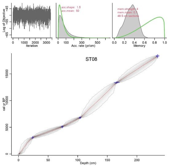
Figure 4.
ST08 age model based on Bayesian approach [77] using rbacon package (version 2.4.2) [78] in R [79]. Upper panels depict the Markov chain Monte Carlo (MCMC) iterations (left panel), the prior (green curves) and posterior (grey histograms) distributions for the accumulation rate (middle panel) and memory (right panel) [78]. Bottom panel shows the calibrated 14C dates (transparent blue) and the age-depth model (darker grays indicate more likely calendar ages, gray stippled lines show 95% confidence intervals, and red curve shows single ‘best’ model based on the mean age for each depth) [78].
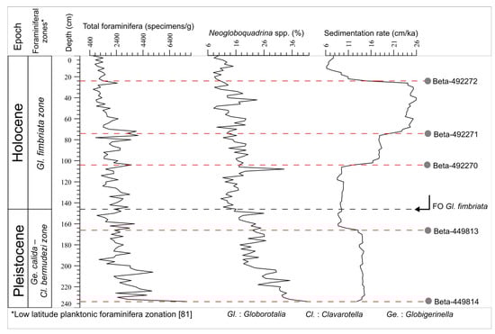
Figure 5.
Sedimentation rates obtained from age model (Table S1) and relevant foraminifera data from previous studies on core ST08 (total foraminifera, Neogloboquadrina spp. abundance, and foraminiferal zones) [56,57] (Table S2). Red dashed lines terminated by gray circles indicate the stratigraphic position of AMS 14C samples. Black dashed line terminated by downwards arrow with tip leftwards indicates the first occurrence (FO) of Gl. fimbriata.
4. Results
4.1. Geochemical Elements and Terrigenous Input Proxies
The intensities of Ti and K show similar trends with less variation in the intensities of Ti in comparison to the intensities of K. Decreases in the intensities of those land-originated elements were detected at ~15–16 (Ti: ~400 ppm, K: ~1400 ppm), ~6–4 (Ti: ~400 ppm, K: ~1600 ppm), and after ~1 ka BP (Ti: ~500 ppm, K:~1500 ppm) while higher intensities were inferred before ~16 ka BP (Ti: ~700 ppm, K:~2400 ppm), at ~13–6 (Ti: ~750 ppm, K: ~2600 ppm) and ~3–1 ka BP (Ti: ~700 ppm, K: ~2400 ppm). The intensities of Ca were relatively high before ~16.5 ka BP (~50,000 ppm), declined at ~16.5–15 ka BP (~20,000 ppm), slightly increased at ~15–1 ka BP (~28,000 ppm) with a peak detected ~6 ka BP (36,000 ppm), and declined after ~1 ka BP (~16,000 ppm) (Figure 6).
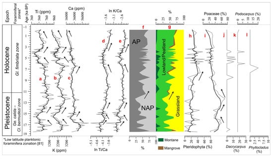
Figure 6.
Geochemical elements obtained from XRF (a–c) and proxies used to infer AIM rainfall ((d,e): terrigenous input proxies, (f–i): pollen and spore proxies) (Tables S3 and S4). Pollen taxa indicating the source area of pollen and spores are also presented (j–l). Data are plotted against the mean ages obtained from the age model. Black curves indicate smoothed values (exponential smoothing).
Terrigenous input proxies (ln Ti/Ca and ln K/Ca) also show similar trends. Their values were relatively low before ~17 ka BP and increased afterward. Slight decreases (still higher than values before ~17 ka BP) were detected ~15–13.5 and ~7–4 ka BP while enhancements were inferred ~17–15, ~13.5–7, and after ~3 ka BP (Figure 6).
4.2. Palynological Proxies (Pollen and Spores)
The records of pollen and spore proxies show less fluctuation compared to the terrigenous input proxies. The abundances of grassland pollen and non-arboreal pollen (NAP) were higher before ~11 ka BP (Last Deglaciation) and declined afterward. Poaceae show a similar trend, but with the addition of a slight decrease in abundance ~16.5–15 ka BP. On the other hand, the abundances of lowland/peatland pollen, mangrove pollen, montane pollen, and arboreal pollen (AP) showed the opposite trend, lower during the Last Deglaciation and increased afterward. The abundance of Pteridophyta was also lower in the Last Deglaciation and increased since ~9 ka BP (Figure 6).
5. Discussion
Results of this study show that the record of terrigenous input proxies is more fluctuating than the record of pollen and spore proxies, which indicate their higher sensitivity to the changes in rainfall. Pollen and spore proxies infer drier condition (lower rainfall) at Last Deglaciation and wetter condition (higher rainfall) at Holocene. Terrigenous input proxies infer three drier periods (i.e., before ~17 and ~15–13.5, and ~7–3 ka), with a more significant rainfall decrease before ~17 ka BP. Three wetter periods (i.e., ~17–15, ~13.5–7, and after ~3 ka BP) are also inferred from these proxies (Figure 7).
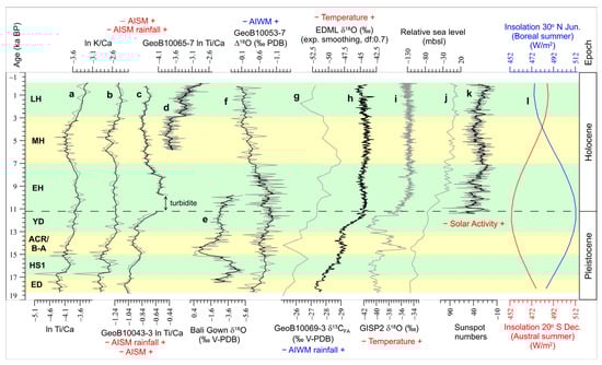
Figure 7.
Drier (yellow highlight) and wetter (green highlight) periods inferred from terrigenous input proxies (a,b). Other paleoclimate records are presented for comparison: (c). Terrigenous input proxy (ln Ti/Ca) record of GeoB10043-3 [10], (d). Terrigenous input proxy (ln Ti/Ca) record of GeoB10065-7 [2], (e). δ18O record of stalagmites from Bali Gown cave (Northwestern Australia) [14], (f). δ18O Globigerinides (Gs.) ruber–δ18O Globigerina (G.) bulloides (Δ18O) record of GeoB10053-7 [1], (g). C30 n-alkanoic fatty acids δ13C (δ13CFA) record of GeoB10069-3 [28], (h). δ18O record of Antarctic (EPICA Dronning Maud Land/EDML) ice core [81], (i). δ18O record of Greenland (GISP2) ice core [82], (j). Reconstructed relative sea level from δ18O of Red sea benthic foraminifera [83,84,85], (k). 10-years averaged reconstructed sunspot numbers [20], and (l). 20° S Dec. (austral summer) insolation (red) and 30° N Jun. (boreal summer) (blue) [21]. Data are plotted against the mean ages obtained from the age model. Black curves indicate smoothed values (exponential smoothing, df: damping factor) (Table S5).
Pollen proxies (i.e., grassland pollen, lowland/peatland pollen, and Poaceae) show similar trends to the oxygen isotope (δ18O) records from the Antarctic [81] and Greenland ice cores [82] that reflect changes in temperature (Figure 8). This indicated that pollen proxies were also sensitive to temperature changes, thus climate during the Last Deglaciation (Holocene) might be characterized by cooler (warmer), and drier (wetter) conditions [71,86,87,88] (Figure 8). Effect of the Last Deglaciation–Holocene temperature changes in the Sumba region was also confirmed by the higher sea surface salinity (SSS) during the Last Deglaciation on the southwestern Savu Sea (near ITF pathway) [72] (Figure 8). The higher (lower) salinity was most likely linked to the weakening (strengthening) of AMOC during the cooler (warmer) Last Deglaciation (Holocene) [72,89]. The weakening of AMOC slowed down the global thermohaline circulation [90,91] and changed the nature (e.g., salinity) of its constituent flows, including ITF [53,92,93]. Pollen proxies did not detect the Last Deglaciation climate events, except Heinrich Stadial 1 (HS1), which were indicated by a decrease in Poaceae abundance (~16.5–15 ka BP) (Figure 8). On the other hand, the increase in Pteridophyta abundance ~9 ka BP was most likely linked to sea-level rise-triggered rainfall increase. The increase in rainfall ~9 ka BP was also indicated by δ18O record from the Liang Luar cave (Flores) [16] and was supported by the high sea level in this period [83,84,85] (Figure 8). The rise of sea level submerged the Indonesian continental shelf, triggering rainfall enhancement through increased moisture supply [6,7]. The lower sensitivity of pollen and spore might be associated with their more extensive source area, which most likely encompassed the Lesser Sunda Islands and Northwestern Australia. Their Lesser Sunda Islands origins were indicated by the occurrence of Podocarpus and Dacrycarpus, typical montane taxa of this region [37,94] (Figure 8). During the Last Deglaciation, the exposed Northwestern Australia shelf could be the additional source area for Poaceae pollen grains, which resulted in its high abundance as its grains easily transported by the winds [36,38,66,95]. The occurrence of Phyllocladus, a typical montane taxon of Australia and New Zealand [66,96], also supports this suggestion (Figure 8). As there were pieces of evidence for the spatial variation of AIM rainfall [5,13,18,28], the changes in AIM rainfall would affect the vegetation (through the changes in drought threshold) not at the same time in each location, so they weakened the pollen and spores-derived signals of monsoon [3,28]. This indicates that pollen and spore proxies are not ideal to reconstruct the past rainfall in this study.
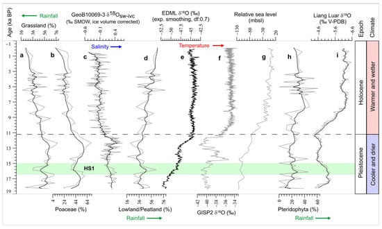
Figure 8.
Last Deglaciation–Holocene climate inferred from palynological (pollen and spores) proxies (a,b,d,h) and other paleoclimate records used for comparison: (c). δ18O seawater with ice volume correction (δ18Osw-ivc) record of GeoB10069-3 [72], (e). δ18O record of Antarctic (EDML) ice core [81], (f). δ18O record of Greenland (GISP2) ice core [82], (g). Reconstructed relative sea level from δ18O of Red sea benthic foraminifera [83,84,85], (i). δ18O record of stalagmites from Liang Luar cave (Flores) [16]. Data are plotted against the mean ages obtained from the age model. Black curves indicate smoothed values (exponential smoothing, df: damping factor) (Table S5).
Terrigenous input proxies infer the variability of riverine runoff related to the changes of rainfall during AISM (AISM rainfall) [1,2,8]. During the Last Deglaciation, the rainfall changes were most likely connected to the high latitude climate events, i.e., early stage of Deglaciation (ED) (before ~17 ka BP), HS1 (~17–15 ka BP), ACR (~15–13.5 ka BP), and Younger Dryas (~13.5–11 ka BP) (Figure 7). Wetter periods coincided with the NH cold events (i.e., HS1 and YD) while drier periods indicated NH warm events (ED) and southern hemisphere (SH) cold events (ACR). [19]. Higher rainfall during HS1 and YD might be induced by the southward shift of the austral summer ITCZ while lower rainfall during ED and ACR were linked to the northward shift of the austral summer ITCZ [8,11] (Figure 9). The NH cooling (during HS1 and YD) enhanced the boreal winter cold surges, which pushed the ITCZ southward [8]. This mechanism also resulted in a southward shift of the boreal summer ITCZ, indicated by the lower EASM rainfall [97,98]. The lower rainfall during ACR could be explained by its co-occurrence with B-A [99] hence the northward shift of austral summer ITCZ was most likely linked to the NH warming (during ED and B-A) [8,19]. The Last Deglaciation rainfall records of ST08 were similar to δ18O records from Bali Gown Cave (Northwestern Australia) [14] (Figure 7), indicating the southern boundary of the austral summer ITCZ during wetter periods (HS1 and YD) [8] (Figure 9). On the other hand, Δ18O (δ18OGs.ruber−δ18OG.bulloides) records (which indicated AIWM changes) from off south Java [1] and terrigenous input proxies (ln Ti/Ca) from off southwest Java [10] showed the opposite rainfall changes during the ACR (Figure 7). This indicated that the records from Java region responded to B-A instead, so they hinted a considerable influence of NH cross-equatorial moisture transport and the southern boundary of the austral summer ITCZ [8] (Figure 9).
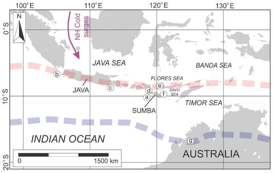
Figure 9.
The southern limit of the austral summer ITCZ during the drier (lower rainfall) periods (red dashed line) and during the wetter (higher) rainfall periods (blue dashed line) as suggested by this study and other previous studies [8,11,100,101]. Numbers show the location of ST08 ((a), this study) and other studies used for comparison i.e., GeoB10043-3 (b) [10], GeoB10053-7 (c) [1], GeoB10065-7 (d) [2], Liang Luar cave (Flores) (e) [16], GeoB10069-3 (f) [28,72], and Bali Gown cave (Northwestern Australia) (g) [14].
The YD wetter period continued until Early Holocene (EH). The abrupt rainfall increase in EH, which was inferred in off southwest Java [10], not detected on ST08. This could be linked to the relatively constant terrigenous input in off southwest Sumba due to the considerable distance from the recently drowned-Sunda Shelf, as opposed to off southwest Java [10]. Δ18O records on off south Java, which changes closely followed boreal summer insolation, increased during YD–EH [1] (Figure 7). This indicated the simultaneous increase of AISM and AIWM, but the effect of the strengthening AIWM and lower austral summer insolation (which should result in AISM weakening) was most likely distressed by the enhanced moisture supply related to abrupt sea-level rise [1,7,10] (Figure 7).
During Mid-Holocene, the rainfall records of ST08 were similar to the ln Ti/Ca records from off northwest Sumba, which inferred drier (wetter) Mid (Late) Holocene [2] (Figure 7). Lower rainfall during the Mid Holocene (MH) (~7–3 ka BP) was most likely linked to the decrease in solar activity (hence lower sunspot numbers) [2,20], which suppressed the effect of increasing austral summer insolation [2,21]. During the Late Holocene (LH) (after ~3 ka BP), an increase in austral summer insolation and solar activity resulted in the enhancement of rainfall [2,20,21]. The southern boundary of the austral summer ITCZ during MH was most likely located around its position during ED and ACR [8,100,101] and shifted southward during LH to around its position during HS1, YD, and EH [2,8,100] (Figure 9), but their relation to solar activity and orbitally-induced austral summer insolation is still not understood [5]. The carbon isotope composition of the C30 n-alkanoic fatty acids (δ13CFA) records from the southwestern Savu Sea [28] showed contradictive rainfall records (Figure 7). This contradiction might be related to the differences in climate signals recorded on terrigenous input and δ13CFA proxies. δ13CFA reflects the dry season (AIWM) water stress connected to the amount of rainfall during AIWM (AIWM rainfall) [28]. We suggest a joint analysis of terrigenous input and δ13CFA proxies from the same site in future studies to reconstruct the past changes of both AISM and AIWM rainfall, so more robust AIM rainfall records are produced.
6. Conclusions
Proxies analyzed in this study (i.e., terrigenous input and pollen and spores) show different sensitivity to AIM rainfall changes since the Last Deglaciation (~18 ka BP). Pollen and spores indicate drier climate during the Last Deglaciation and wetter climate during the Holocene. Terrigenous input proxies are more sensitive as they can detect three drier periods (i.e., before ~17, ~15–13.5, and 7–3 ka BP) and three wetter periods (i.e., ~17–15, ~13.5–7, and after ~3 ka BP) which represent the AISM rainfall changes. The lower sensitivity of pollen and spore proxies was related to their wider source area (the Lesser Sunda Islands and Northwestern Australia). This might be the reason of the absence of high latitude climatic event signals (i.e., ED, HS1, ACR, and YD) in nearly all pollen and spore proxies (except Poaceae) despite their high responsiveness to temperature changes. During the Last Deglaciation, AISM rainfall changes indicated a strong response to high latitude climatic events. The higher rainfall periods were linked to the southward shift of the austral summer ITCZ during the NH cold events (i.e., HS1 and YD) while the northward shift of the austral summer ITCZ resulted in lower AISM rainfall during the NH warm event (ED) and SH cold event (ACR, coeval with B-A). AISM rainfall changes during the Holocene were related to the sea-level rise (EH), solar activity (MH and LH), and orbitally-induced austral summer insolation (LH). Differences in recorded climate signals caused the contradiction between our AISM rainfall records and the rainfall records from the southwestern Savu Sea (which inferred AIWM rainfall). A joint analysis of terrigenous input and δ13CFA proxies from the same site is suggested in future studies to develop more robust AIM rainfall records.
Supplementary Materials
The following are available online at https://www.mdpi.com/2073-4433/11/9/932/s1, Table S1: Sedimentation rates, Table S2: ST08 total foraminifera and the abundance of Neogloboquadrina spp., Table S3: ST08 XRF-based geochemical element data, Table S4: ST08 palynological proxies (pollen and spores), Table S5: Smoothed values of paleoclimate records presented in Figure 7 and Figure 8. The insolation, sunspot numbers, and paleoclimate data used for comparison in this study are available at https://www.ncdc.noaa.gov/paleo-search/ and https://www.pangaea.de/. The bathymetry data from GEBCO Bathymetric Compilation Group 2020 are available at https://www.gebco.net/data_and_products/gridded_bathymetry_data/.
Author Contributions
Conceptualization, R.D.W.A.; Data curation, R.D.W.A.; Formal analysis, R.D.W.A. and I.; Funding acquisition, R.D.W.A., P.S.P. and S.H.N.; Investigation, R.D.W.A.; Methodology, R.D.W.A., A. and K.A.M.; Project administration, P.S.P. and S.H.N.; Resources, A., K.A.M. and E.Y.; Software, R.D.W.A.; Supervision, A., K.A.M., and E.Y.; Validation, A., K.A.M. and E.Y.; Visualization, R.D.W.A.; Writing—original draft, R.D.W.A.; Writing—review & editing, R.D.W.A., P.S.P. and S.H.N. All authors have read and agreed to the published version of the manuscript.
Funding
This research was funded by the Indonesian Endowment Fund for Education (LPDP) (grant number 202001110215954) and the Research Center for Oceanography of LIPI. Furthermore, The APC was funded by the Indonesian Endowment Fund for Education (LPDP).
Acknowledgments
We thank the Indonesian Endowment Fund for Education (LPDP) for the financial aid. We thank the Research Center for Oceanography of LIPI, especially Udhi Hermawan, as the chief scientist of E-WIN 2016 for the permission of data usage and administrative assistance. We thank Singgih Prasetyo Adi Wibowo and all crews of the Baruna Jaya VIII R.V. for technical supports and data collecting. The Research Center for Geotechnology of LIPI and the Geological Engineering Study Program of Institut Teknologi Bandung (ITB) are thanked for the laboratory facilities.
Conflicts of Interest
The authors declare no conflict of interest. The funders had no role in the design of the study; in the collection, analyses, or interpretation of data; in the writing of the manuscript, or in the decision to publish the results.
References
- Mohtadi, M.; Oppo, D.W.; Steinke, S.; Stuut, J.B.W.; De Pol-Holz, R.; Hebbeln, D.; Lückge, A. Glacial to Holocene swings of the Australian-Indonesian monsoon. Nat. Geosci. 2011, 4, 540–544. [Google Scholar] [CrossRef]
- Steinke, S.; Mohtadi, M.; Prange, M.; Varma, V.; Pittauerova, D.; Fischer, H.W. Mid-to late-Holocene australian-indonesian summer monsoon variability. Quat. Sci. Rev. 2014, 93, 142–154. [Google Scholar] [CrossRef]
- Wicaksono, S.A.; Russell, J.M.; Holbourn, A.; Kuhnt, W. Hydrological and vegetation shifts in the Wallacean region of central Indonesia since the Last Glacial Maximum. Quat. Sci. Rev. 2017, 157, 152–163. [Google Scholar] [CrossRef]
- Mohtadi, M.; Prange, M.; Steinke, S. Palaeoclimatic insights into forcing and response of monsoon rainfall. Nature 2016, 533, 191–199. [Google Scholar] [CrossRef] [PubMed]
- Steinke, S.; Prange, M.; Feist, C.; Groeneveld, J.; Mohtadi, M. Upwelling variability off southern Indonesia over the past two millennia. Geophys. Res. Lett. 2014, 41, 7684–7693. [Google Scholar] [CrossRef]
- Griffiths, M.L.; Drysdale, R.N.; Gagan, M.K.; Frisia, S.; Zhao, J.X.; Ayliffe, L.K.; Hantoro, W.S.; Hellstrom, J.C.; Fischer, M.J.; Feng, Y.X.; et al. Evidence for Holocene changes in australian-indonesian monsoon rainfall from stalagmite trace element and stable isotope ratios. Earth Planet. Sci. Lett. 2010, 292, 27–38. [Google Scholar] [CrossRef]
- Griffiths, M.L.; Drysdale, R.N.; Gagan, M.K.; Zhao, J.X.; Ayliffe, L.K.; Hellstrom, J.C.; Hantoro, W.S.; Frisia, S.; Feng, Y.X.; Cartwright, I.; et al. Increasing australian-indonesian monsoon rainfall linked to early Holocene sea-level rise. Nat. Geosci. 2009, 2, 636–639. [Google Scholar] [CrossRef]
- Kuhnt, W.; Holbourn, A.; Xu, J.; Opdyke, B.; De Deckker, P.; Mudelsee, M. Southern hemisphere control on australian monsoon variability during the late deglaciation and Holocene. Nat. Commun. 2015. [Google Scholar] [CrossRef]
- Liu, S.; Zhang, H.; Shi, X.; Chen, M.; Cao, P.; Li, Z.; Troa, R.A.; Zuraida, R.; Triarso, E.; Marfasran, H. Reconstruction of monsoon evolution in southernmost Sumatra over the past 35 kyr and its response to northern hemisphere climate changes. Prog. Earth Planet. Sci. 2020, 7, 30. [Google Scholar] [CrossRef]
- Setiawan, R.Y.; Mohtadi, M.; Southon, J.; Groeneveld, J.; Steinke, S.; Hebbeln, D. The consequences of opening the Sunda Strait on the hydrography of the eastern tropical Indian Ocean. Paleoceanography 2015, 30, 1358–1372. [Google Scholar] [CrossRef]
- Ding, X.; Bassinot, F.; Guichard, F.; Fang, N.Q. Indonesian Throughflow and monsoon activity records in the Timor Sea since the last glacial maximum. Mar. Micropaleontol. 2013, 101, 115–126. [Google Scholar] [CrossRef]
- Spooner, M.I.; Barrows, T.T.; De Deckker, P.; Paterne, M. Palaeoceanography of the Banda Sea, and Late Pleistocene initiation of the Northwest Monsoon. Glob. Planet. Chang. 2005, 49, 28–46. [Google Scholar] [CrossRef]
- Wyrwoll, K.H.; Miller, G.H. Initiation of the Australian summer monsoon 14,000 years ago. Quat. Int. 2001, 82, 119–128. [Google Scholar] [CrossRef]
- Denniston, R.F.; Wyrwoll, K.H.; Asmerom, Y.; Polyak, V.J.; Humphreys, W.F.; Cugley, J.; Woods, D.; LaPointe, Z.; Peota, J.; Greaves, E. North Atlantic forcing of millennial-scale indo-australian monsoon dynamics during the Last Glacial period. Quat. Sci. Rev. 2013, 72, 159–168. [Google Scholar] [CrossRef]
- Wang, P.X.; Wang, B.; Cheng, H.; Fasullo, J.; Guo, Z.; Kiefer, T. The global monsoon across time scales: Mechanisms and outstanding issues. Earth Sci. Rev. 2017, 174, 84–121. [Google Scholar] [CrossRef]
- Ayliffe, L.K.; Gagan, M.K.; Zhao, J.; Drysdale, R.N.; Hellstrom, J.C.; Hantoro, W.S.; Griffiths, M.L.; Scott-gagan, H.; Pierre, E.S.; Cowley, J.A.; et al. Australasian monsoon during the last deglaciation. Nat. Commun. 2013, 4, 1–6. [Google Scholar] [CrossRef] [PubMed]
- Magee, J.W.; Miller, G.H.; Spooner, N.A.; Questiaux, D. Continuous 150 k.y. monsoon record from Lake Eyre, Australia: Insolation-forcing implications and unexpected Holocene failure. Geology 2004, 32, 885–888. [Google Scholar] [CrossRef]
- Nott, J.; Price, D. Plunge pools and paleoprecipitation. Geology 1994, 22, 1047–1050. [Google Scholar] [CrossRef]
- Denniston, R.F.; Wyrwoll, K.; Polyak, V.J.; Brown, J.R.; Asmerom, Y.; Wanamaker, A.D.; Lapointe, Z.; Ellerbroek, R.; Barthelmes, M.; Cleary, D.; et al. A stalagmite record of Holocene indonesian e australian summer monsoon variability from the australian tropics. Quat. Sci. Rev. 2013, 78, 155–168. [Google Scholar] [CrossRef]
- Solanki, S.K.; Usoskin, I.G.; Kromer, B.; Schüssler, M.; Beer, J. Unusual activity of the Sun during recent decades compared to the previous 11,000 years. Nature 2004, 431, 1084–1087. [Google Scholar] [CrossRef]
- Berger, A.L. Long-term variations of daily insolation and Quaternary climatic changes. J. Atmos. Sci. 1978, 35, 2361–2367. [Google Scholar] [CrossRef]
- Berger, A.; Loutre, M.F. Insolation values for the climate of the last 10 million years. Quat. Sci. Rev. 1991, 10, 297–317. [Google Scholar] [CrossRef]
- Meehl, G.A.; Washington, W.M.; Wigley, T.M.L.; Arblaster, J.M.; Dai, A. Solar and greenhouse gas forcing and climate response in the twentieth century. J. Clim. 2003, 16, 426–444. [Google Scholar] [CrossRef]
- Hanebuth, T.J.J.; Voris, H.K.; Yokoyama, Y.; Saito, Y.; Okuno, J. Formation and fate of sedimentary depocentres on southeast Asia’s Sunda Shelf over the past sea-level cycle and biogeographic implications. Earth Sci. Rev. 2011, 104, 92–110. [Google Scholar] [CrossRef]
- Broecker, W.S. Paleocean circulation during the last deglaciation: A bipolar seesaw? Paleoceanography 1998, 13, 119–121. [Google Scholar] [CrossRef]
- Stocker, T.F.; Johnsen, S.J. A minimum thermodynamic model for the bipolar seesaw. Paleoceanography 2003, 18, 1–9. [Google Scholar] [CrossRef]
- Aldrian, E.; Susanto, R.D. Identification of three dominant rainfall regions within Indonesia and their relationship to sea surface temperature. Int. J. Climatol. 2003, 23, 1435–1452. [Google Scholar] [CrossRef]
- Dubois, N.; Oppo, D.W.; Galy, V.V.; Mohtadi, M.; Van Der Kaars, S.; Tierney, J.E.; Rosenthal, Y.; Eglinton, T.I.; Lückge, A.; Linsley, B.K. Indonesian vegetation response to changes in rainfall seasonality over the past 25,000 years. Nat. Geosci. 2014, 7, 513–517. [Google Scholar] [CrossRef]
- Rixen, T.; Ittekkot, V.; Herunadi, B.; Wetzel, P.; Maier-Reimer, E.; Gaye-Haake, B. ENSO-driven carbon see saw in the Indo-Pacific. Geophys. Res. Lett. 2006, 33, L07606. [Google Scholar] [CrossRef]
- Weltje, G.J.; Tjallingii, R. Calibration of XRF core scanners for quantitative geochemical logging of sediment cores: Theory and application. Earth Planet. Sci. Lett. 2008, 274, 423–438. [Google Scholar] [CrossRef]
- Calvert, S.E.; Pedersen, T.F. Elemental proxies for Palaeoclimatic and Palaeoceanographic variability in marine sediments: Interpretation and application. In Developments in Marine Geology; Elsevier: Amsterdam, The Netherlands, 2007; Volume 1, pp. 567–644. ISBN 9780444527554. [Google Scholar]
- Croudace, I.W.; Rindby, A.; Rothwell, R.G. ITRAX: Description and evaluation of a new multi-function X-ray core scanner. Geol. Soc. Spec. Publ. 2006, 267, 51–63. [Google Scholar] [CrossRef]
- Richter, T.O.; Van Der Gaast, S.; Koster, B.; Vaars, A.; Gieles, R.; De Stigter, H.C.; De Haas, H.; Van Weering, T.C.E. The Avaatech XRF Core scanner: Technical description and applications to NE Atlantic sediments. Geol. Soc. Spec. Publ. 2006, 267, 39–50. [Google Scholar] [CrossRef]
- Dypvik, H.; Harris, N.B. Geochemical facies analysis of fine-grained siliciclastics using Th/U, Zr/Rb and (Zr + Rb)/Sr ratios. Chem. Geol. 2001, 181, 131–146. [Google Scholar] [CrossRef]
- Aitchison, J. The Statistical Analysis of Compositional Data. J. R. Stat. Soc. Ser. B 1982, 44, 139–160. [Google Scholar] [CrossRef]
- van der Kaars, W.A. Palynology of eastern indonesian marine piston-cores: A late Quaternary vegetational and climatic record for Australasia. Palaeogeogr. Palaeoclimatol. Palaeoecol. 1991, 85. [Google Scholar] [CrossRef]
- Wang, X.; Van Der Kaars, S.; Kershaw, P.; Bird, M.; Jansen, F. A record of fire, vegetation and climate through the last three glacial cycles from Lombok Ridge core G6-4, eastern Indian Ocean, Indonesia. Palaeogeogr. Palaeoclimatol. Palaeoecol. 1999, 147, 241–256. [Google Scholar] [CrossRef]
- Van Der Kaars, S.; Wang, X.; Kershaw, P.; Guichard, F.; Setiabudi, D.A. A late Quaternary palaeoecological record from the Banda Sea, Indonesia: Patterns of vegetation, climate and biomass burning in Indonesia and northern Australia. Palaeogeogr. Palaeoclimatol. Palaeoecol. 2000, 155, 135–143. [Google Scholar] [CrossRef]
- Barmawidjaja, B.M.; Rohling, E.J.; van der Kaars, W.A.; Vergnaud Grazzini, C.; Zachariasse, W.J. Glacial conditions in the northern Molucca Sea region (Indonesia). Palaeogeogr. Palaeoclimatol. Palaeoecol. 1993, 101, 147–167. [Google Scholar] [CrossRef]
- Yulianto, E.; Rahardjo, A.T.; Noeradi, D.; Siregar, D.A.; Hirakawa, K. A Holocene pollen record of vegetation and coastal environmental changes in the coastal swamp forest at Batulicin, South Kalimantan, Indonesia. J. Asian Earth Sci. 2005, 25, 1–8. [Google Scholar] [CrossRef]
- Huang, E.; Tian, J.; Liu, J. Dynamics of the australian-indonesian monsoon across termination II: Implications of molecular-biomarker reconstructions from the Timor Sea. Palaeogeogr. Palaeoclimatol. Palaeoecol. 2015, 423, 32–43. [Google Scholar] [CrossRef]
- Wang, B.; Liu, J.; Kim, H.-J.; Webster, P.J.; Yim, S.-Y. Recent change of the global monsoon precipitation (1979–2008). Clim. Dyn. 2012, 39, 1123–1135. [Google Scholar] [CrossRef]
- Wang, H.; Chen, J.; Zhang, X.; Chen, F. Palaeosol development in the Chinese Loess Plateau as an indicator of the strength of the east Asian summer monsoon: Evidence for a mid-Holocene maximum. Quat. Int. 2014, 334–335, 155–164. [Google Scholar] [CrossRef]
- Wheeler, M.C.; McBride, J.L. Australian-indonesian monsoon. In Intraseasonal Variability in the Atmosphere-Ocean Climate System; Springer: Berlin/Heidelberg, Germany, 2005; pp. 125–173. [Google Scholar]
- Mohtadi, M.; Max, L.; Hebbeln, D.; Baumgart, A.; Krück, N.; Jennerjahn, T. Modern environmental conditions recorded in surface sediment samples off W and SW Indonesia: Planktonic foraminifera and biogenic compounds analyses. Mar. Micropaleontol. 2007, 65, 96–112. [Google Scholar] [CrossRef]
- Suppiah, R.; Wu, X. Surges, cross-equatorial flows and their links with the australian summer monsoon circulation and rainfall. Aust. Meteorol. Mag. 1998, 47, 113–130. [Google Scholar]
- Tomczak, M.; Godfrey, J.S. Adjacent seas of the Indian Ocean and the Australasian Mediterranian Sea (The indonesian throughflow). In Regional Oceanography: An Introduction; Daya Publishing House: New Delhi, India, 2003; pp. 215–228. [Google Scholar]
- Qu, T.; Du, Y.; Strachan, J.; Meyers, G.; Slingo, J. Sea surface temperature and its variability in the indonesian region. Oceanography 2005, 18, 50–61. [Google Scholar] [CrossRef]
- Poliakova, A.; Rixen, T.; Jennerjahn, T.; Behling, H. Eleven month high resolution pollen and spore sedimentation record off SW Java in the Indian Ocean. Mar. Micropaleontol. 2014, 111, 90–99. [Google Scholar] [CrossRef]
- Gordon, A. Oceanography of the indonesian seas and their throughflow. Oceanography 2005, 18, 14–27. [Google Scholar] [CrossRef]
- Xu, J. Change of indonesian throughflow outflow in response to east asian monsoon and ENSO activities since the Last Glacial. Sci. China Earth Sci. 2014, 57, 791–801. [Google Scholar] [CrossRef]
- Xu, J.; Holbourn, A.; Kuhnt, W.; Jian, Z.; Kawamura, H. Changes in the thermocline structure of the indonesian out flow during terminations I and II. Earth Planet. Sci. Lett. 2008, 273, 152–162. [Google Scholar] [CrossRef]
- Holbourn, A.; Kuhnt, W.; Xu, J. Indonesian throughflow variability during the last 140 ka: The timor sea outflow. Geol. Soc. Spec. Publ. 2011, 355, 283–303. [Google Scholar] [CrossRef]
- Putra, P.S.; Nugroho, S.H. Holocene climate dynamics in Sumba Strait, Indonesia: A preliminary evidence from high resolution geochemical records and planktonic foraminifera. Stud. Quartenaria. (in press).
- Bayhaqi, A.; Lenn, Y.-D.; Surinati, D.; Polton, J.; Nur, M.; Corvianawatie, C.; Purwandana, A. The variability of indonesian throughflow in Sumba Strait and its linkage to the climate events. Am. J. Appl. Sci. 2019, 16, 118–133. [Google Scholar] [CrossRef][Green Version]
- Ardi, R.D.W. Paleoclimatology and Paleo-Oceanography Reconstruction since Late Pleistocene Based on Foraminifera Assemblages Off the Southwest Coast of Sumba Island, East Nusa Tenggara. Master’s Thesis, Institut Teknologi, Bandung, Indonesia, 2018. [Google Scholar]
- Ardi, R.D.W.; Maryunani, K.A.; Yulianto, E.; Putra, P.S.; Nugroho, S.H. Biostratigraphy and analysis of changes in thermocline depth off the Southwest Coast of Sumba since the Late Pleistocene based on planktonic foraminifera assemblages. Bull. Geol. 2019, 3, 355–362. [Google Scholar] [CrossRef]
- Hemming, S.R. Terrigenous sediments. In Paleoceanography, Physical and Chemical Proxies; Elsevier: Amsterdam, The Netherlands, 2007; pp. 1776–1786. ISBN 9780444536433. [Google Scholar]
- Kissel, C.; Laj, C.; Kienast, M.; Bolliet, T.; Holbourn, A.; Hill, P.; Kuhnt, W.; Braconnot, P. Monsoon variability and deep oceanic circulation in the western equatorial Pacific over the last climatic cycle: Insights from sedimentary magnetic properties and sortable silt. Paleoceanography 2010, 25, 1–12. [Google Scholar] [CrossRef]
- Nesbitt, H.W.; Markovics, G.; Price, R.C. Chemical processes affecting alkalis and alkaline earths during continental weathering. Geochim. Cosmochim. Acta 1980, 44, 1659–1666. [Google Scholar] [CrossRef]
- Langer, M.R. Assessing the contribution of foraminiferan protists to global ocean carbonate production. J. Eukaryot. Microbiol. 2008, 55, 163–169. [Google Scholar] [CrossRef]
- Fortuin, A.R.; Roep, T.B.; Sumosusastro, P.A. The Neogene sediments of east Sumba, Indonesia-products of a lost arc? J. Southeast Asian Earth Sci. 1994, 9, 67–79. [Google Scholar] [CrossRef]
- Abdullah, C.I.; Rampnoux, J.P.; Bellon, H.; Maury, R.C.; Soeria-Atmadja, R. The evolution of Sumba Island (Indonesia) revisited in the light of new data on the geochronology and geochemistry of the magmatic rocks. J. Asian Earth Sci. 2000, 18, 533–546. [Google Scholar] [CrossRef]
- Hu, D.; Böning, P.; Köhler, C.M.; Hillier, S.; Pressling, N.; Wan, S.; Brumsack, H.J.; Clift, P.D. Deep sea records of the continental weathering and erosion response to east Asian monsoon intensification since 14 ka in the South China Sea. Chem. Geol. 2012, 326–327, 1–18. [Google Scholar] [CrossRef]
- Liu, B.; Wang, Y.; Su, X.; Zheng, H. Elemental geochemistry of northern slope sediments from the South China Sea: Implications for provenance and source area weathering since Early Miocene. Chem. Erde Geochem. 2013, 73, 61–74. [Google Scholar] [CrossRef]
- Istiana. Characteristics of palynomorph due to climate change in deep sea sediment since the Late Pleistocene, East Nusa Tenggara. Master’s Thesis, Institut Teknologi Bandung, Indonesia, 2019. [Google Scholar]
- Hesse, M.; Waha, M. A new look at the acetolysis method. Plant Syst. Evol. 1989, 163, 147–152. [Google Scholar] [CrossRef]
- Yulianto, E.; Sukapti, W.S.; Rahardjo, A.T.; Noeradi, D.; Siregar, D.A.; Suparan, P.; Hirakawa, K. Mangrove shoreline responses to Holocene environmental change, Makassar Strait, Indonesia. Rev. Palaeobot. Palynol. 2004, 131, 251–268. [Google Scholar] [CrossRef]
- Haberle, S.; Rowe, C.; Hungerford, S.; Preston, T.; Warren, P.; Hope, G.; Hopf, F.; Thornhill, A.; Stevenson, J.; Weng, C.; et al. The Australasian Pollen and Spore Atlas V1.0. Available online: http://apsa.anu.edu.au/ (accessed on 20 September 2001).
- Johns, R.J. Plant zonation. In Biogeography and Ecology of New Guinea. Monographiae Biologicae; Gressit, J.L., Ed.; Springer: Dordrecht, The Netherlands, 1982; pp. 309–330. [Google Scholar]
- Van Der Kaars, S.; Penny, D.; Tibby, J.; Fluin, J.; Dam, R.A.C.; Suparan, P. Late quaternary palaeoecology, palynology and palaeolimnology of a tropical lowland swamp: Rawa Danau, West-Java, Indonesia. Palaeogeogr. Palaeoclimatol. Palaeoecol. 2001, 171, 185–212. [Google Scholar] [CrossRef]
- Gibbons, F.T.; Oppo, D.W.; Mohtadi, M.; Rosenthal, Y.; Cheng, J.; Liu, Z.; Linsley, B.K. Deglacial δ18O and hydrologic variability in the tropical Pacific and Indian Oceans. Earth Planet. Sci. Lett. 2014, 387, 240–251. [Google Scholar] [CrossRef]
- GEBCO Bathymetric Compilation Group 2020. GEBCO_2020 Grid. 2020. [Google Scholar]
- Bronk Ramsey, C. Bayesian analysis of radiocarbon dates. Radiocarbon 2009, 51, 337–360. [Google Scholar] [CrossRef]
- Reimer, P.J.; Edouard Bard, B.; Alex Bayliss, B.; Warren Beck, B.J.; Paul Blackwell, B.G.; Christopher Bronk Ramsey, B. Intcal13 and Marine13 radiocarbon age calibration curves 0–50,000 years Cal Bp. Radiocarbon 2013, 55, 1869–1887. [Google Scholar] [CrossRef]
- Talma, A.S.; Vogel, J.C. A simplified approach to calibrating 14C dates. Radiocarbon 1993, 35, 317–322. [Google Scholar] [CrossRef]
- Blaauw, M.; Christeny, J.A. Flexible paleoclimate age-depth models using an autoregressive gamma process. Bayesian Anal. 2011, 6, 457–474. [Google Scholar] [CrossRef]
- Blaauw, M.; Christen, J.A.; Aquino, M.A. rbacon: Age-Depth Modelling Using Bayesian Statistics. R. Packag. Version 2.4.2. 2020. Available online: https://cran.r-project.org/web/packages/rbacon/rbacon.pdf (accessed on 26 July 2020).
- R Core Team. R: A language and Environment for Statistical Computing; R Foundation for Statistical Computing: Vienna, Austria, 2013. [Google Scholar]
- Bolli, H.M.; Saunders, J.B. Oligocene to Holocene low latitude planktic foraminifera. In Plankton Stratigraphy; Bolli, H.M., Saunders, J.B., Perch-Nielsen, K., Eds.; Cambridge University Press: New York, NY, USA, 1985; pp. 155–262. ISBN 978-0-521-36719-6. [Google Scholar]
- Augustin, L.; Barbante, C.; Barnes, P.R.; Barnola, J.M.; Bigler, M.; Castellano, E.; Cattani, O.; Chappellaz, J.; Dahl-Jensen, D.; Delmonte, B.; et al. One-to-one coupling of glacial climate variability in Greenland and Antarctica. Nature 2006, 444, 195–198. [Google Scholar] [CrossRef]
- Grootes, P.M.; Stuiver, M. Oxygen 18/16 variability in Greenland snow and ice with 10−3-to 10 5-year time resolution. J. Geophys. Res. Ocean. 1997, 102, 26455–26470. [Google Scholar] [CrossRef]
- Siddall, M.; Rohling, E.J.; Almogi-Labin, A.; Hemleben, C.; Meischner, D.; Schmelzer, I.; Smeed, D.A. Sea-level fluctuations during the last glacial cycle. Nature 2003, 423, 853–858. [Google Scholar] [CrossRef] [PubMed]
- Arz, H.W.; Lamy, F.; Ganopolski, A.; Nowaczyk, N.; Pätzold, J. Dominant Northern Hemisphere climate control over millennial-scale glacial sea-level variability. Quat. Sci. Rev. 2007, 26, 312–321. [Google Scholar] [CrossRef]
- Siddall, M. Red Sea Level Reconstruction. IGBP PAGES/World Data Center for Paleoclimatology Data Contribution Series # 2006-063. NOAA/NCDC; Paleoclimatology Program: Boulder, CO, USA, 2006. [Google Scholar]
- Stuitjs, I.; Newsome, J.; Flenley, J.R. Evidence for Late Quaternary vegetational change. Rev. Palaeobot. Palynol. 1988, 55, 207–216. [Google Scholar]
- Hope, G.; Tulip, J. A long vegetation history from lowland Irian Jaya, Indonesia. Palaeogeogr. Palaeoclimatol. Palaeoecol. 1994, 109, 385–398. [Google Scholar] [CrossRef]
- Yosephin, Y.; Nugroho, S.H.; Putra, P.S.; Suedy, S.W.A.; Izzati, M. Palinologi Laut di Selat Sumba, Nusa Tenggara Timur. Ris. Geol. Pertamb. 2019, 29, 43. [Google Scholar] [CrossRef]
- Levi, C.; Labeyrie, L.; Bassinot, F.; Guichard, F.; Cortijo, E.; Waelbroeck, C.; Caillon, N.; Duprat, J.; de Garidel-Thoron, T.; Elderfield, H. Low-latitude hydrological cycle and rapid climate changes during the last deglaciation. Geochem. Geophys. Geosyst. 2007, 8. [Google Scholar] [CrossRef]
- Lynch-Stieglitz, J.; Schmidt, M.W.; Gene Henry, L.; Curry, W.B.; Skinner, L.C.; Mulitza, S.; Zhang, R.; Chang, P. Muted change in Atlantic overturning circulation over some glacial-aged Heinrich events. Nat. Geosci. 2014, 7, 144–150. [Google Scholar] [CrossRef]
- Deplazes, G.; Lückge, A.; Peterson, L.C.; Timmermann, A.; Hamann, Y.; Hughen, K.A.; Röhl, U.; Laj, C.; Cane, M.A.; Sigman, D.M.; et al. Links between tropical rainfall and North Atlantic climate during the last glacial period. Nat. Geosci. 2013, 6, 213–217. [Google Scholar] [CrossRef]
- Xu, J.; Kuhnt, W.; Holbourn, A.; Andersen, N.; Bartoli, G. Changes in the vertical profile of Indonesian Throughflow during Termination II: Evidence from the Timor Sea. Paleoceanography 2006, 21, 1–14. [Google Scholar] [CrossRef]
- Kuhnt, W.; Holbourn, A.; Hall, R.; Zuvela, M.; Käse, R. Neogene history of the indonesian throughflow. In Geophysical Monograph Series; American Geophysical Union: Washington, DC, USA, 2004; Volume 149, pp. 299–320. ISBN 9781118666067. [Google Scholar]
- Morley, R.J. Palynological evidence for Tertiary plant dispersals in the SE Asian region in relation to plate tectonics and climate. Biogeogr. Geol. Evol. SE Asia 1998, 34, 211–234. [Google Scholar]
- Van Der Kaars, S.; Deckker, P. De A Late Quaternary pollen record from deep-sea core Fr10/95, GC17 offshore Cape Range Peninsula, northwestern western Australia. Rev. Palaeobot. Palynol. 2002, 120, 17–39. [Google Scholar] [CrossRef]
- Wagstaff, S.J. Evolution and biogeography of the austral genus Phyllocladus (Podocarpaceae). J. Biogeogr. 2004, 31, 1569–1577. [Google Scholar] [CrossRef]
- Lu, H.; Yi, S.; Liu, Z.; Mason, J.A.; Jiang, D.; Cheng, J.; Xu, Z.; Zhang, E.; Jin, L.; Zhang, Z.; et al. Variation of east asian monsoon precipitation during the past 21 k.y. and potential CO2 forcing. Geology 2013. [Google Scholar] [CrossRef]
- Wu, H.N.; Ma, Y.Z.; Feng, Z.; Sun, A.Z.; Zhang, C.J.; Li, F.; Kuang, J. A high resolution record of vegetation and environmental variation through the last∼ 25,000 years in the western part of the Chinese Loess Plateau. Palaeogeogr. Palaeoclimatol. Palaeoecol. 2009, 273, 191–199. [Google Scholar] [CrossRef]
- Morgan, V.I. Antarctic cold reversal. In Encyclopedia of Paleoclimatology and Ancient Environments; Springer: Dordrecht, The Netherlands, 2009; pp. 22–24. [Google Scholar]
- Tierney, J.E.; Oppo, D.W.; Rosenthal, Y.; Russell, J.M.; Linsley, B.K. Coordinated hydrological regimes in the Indo-Pacific region during the past two millennia. Paleoceanography 2010, 25, 1–7. [Google Scholar] [CrossRef]
- Ishiwa, T.; Yokoyama, Y.; Reuning, L.; McHugh, C.M.; De Vleeschouwer, D.; Gallagher, S.J. Australian summer monsoon variability in the past 14,000 years revealed by IODP expedition 356 sediments. Prog. Earth Planet. Sci. 2019, 6. [Google Scholar] [CrossRef]


© 2020 by the authors. Licensee MDPI, Basel, Switzerland. This article is an open access article distributed under the terms and conditions of the Creative Commons Attribution (CC BY) license (http://creativecommons.org/licenses/by/4.0/).