Observations of Emissions and the Influence of Meteorological Conditions during Wildfires: A Case Study in the USA, Brazil, and Australia during the 2018/19 Period


Abstract
:1. Introduction
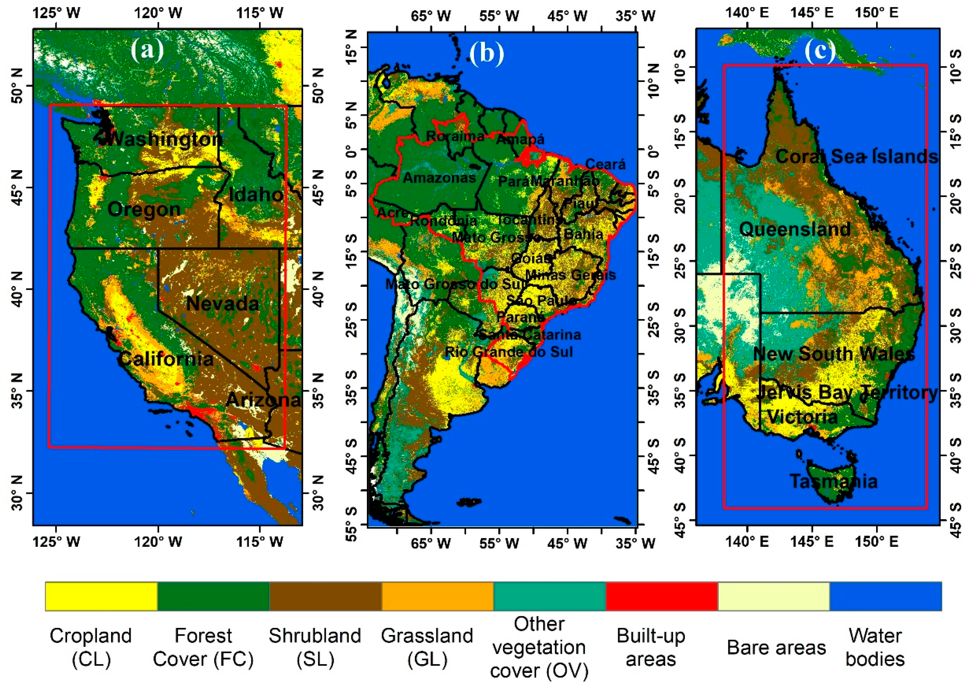
2. Study Sites
3. Data and Methods
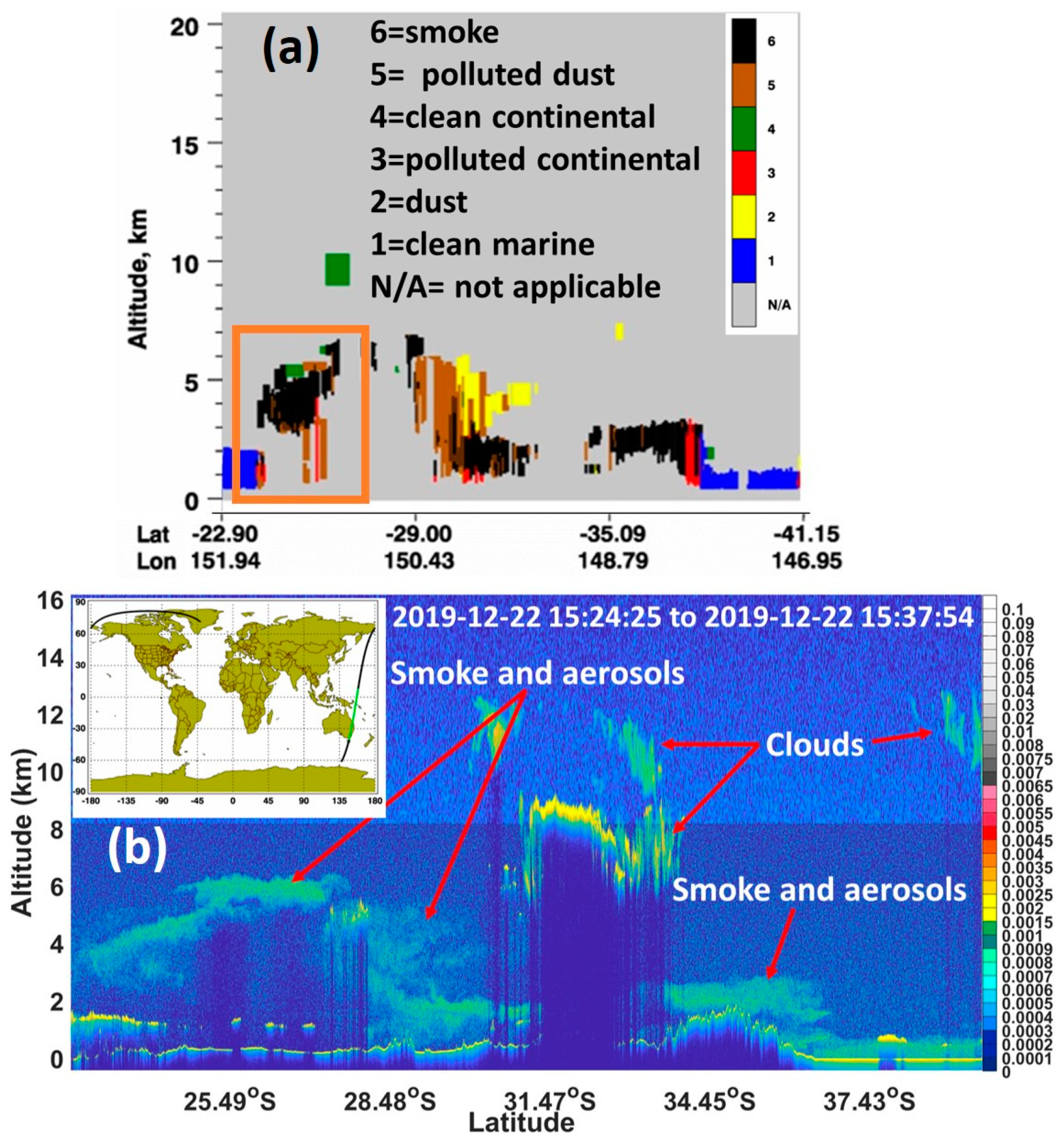
3.1. CALIPSO
3.2. Sentinel-5 Precursor (5P)
3.3. MERRA-2
3.4. AIRS
4. Results
4.1. Observation of the Atmospheric Pollutants from Wildfires
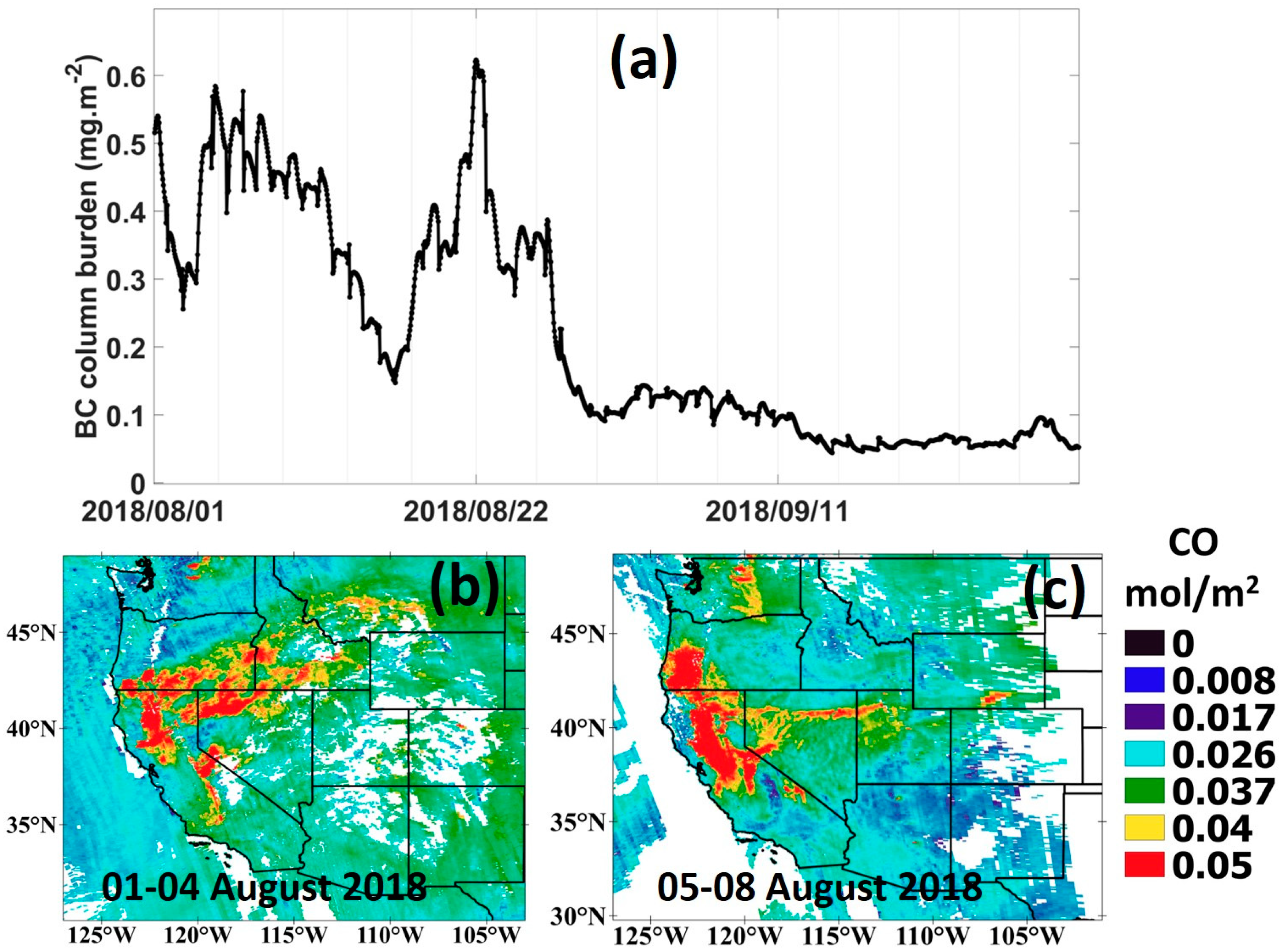
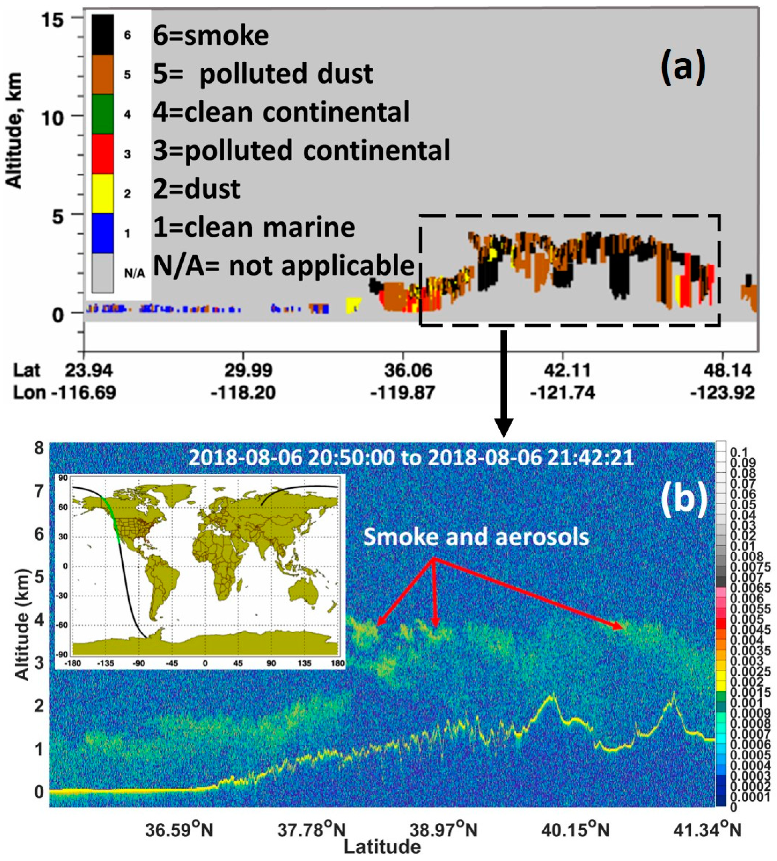
4.1.1. USA Fires (August 2018)
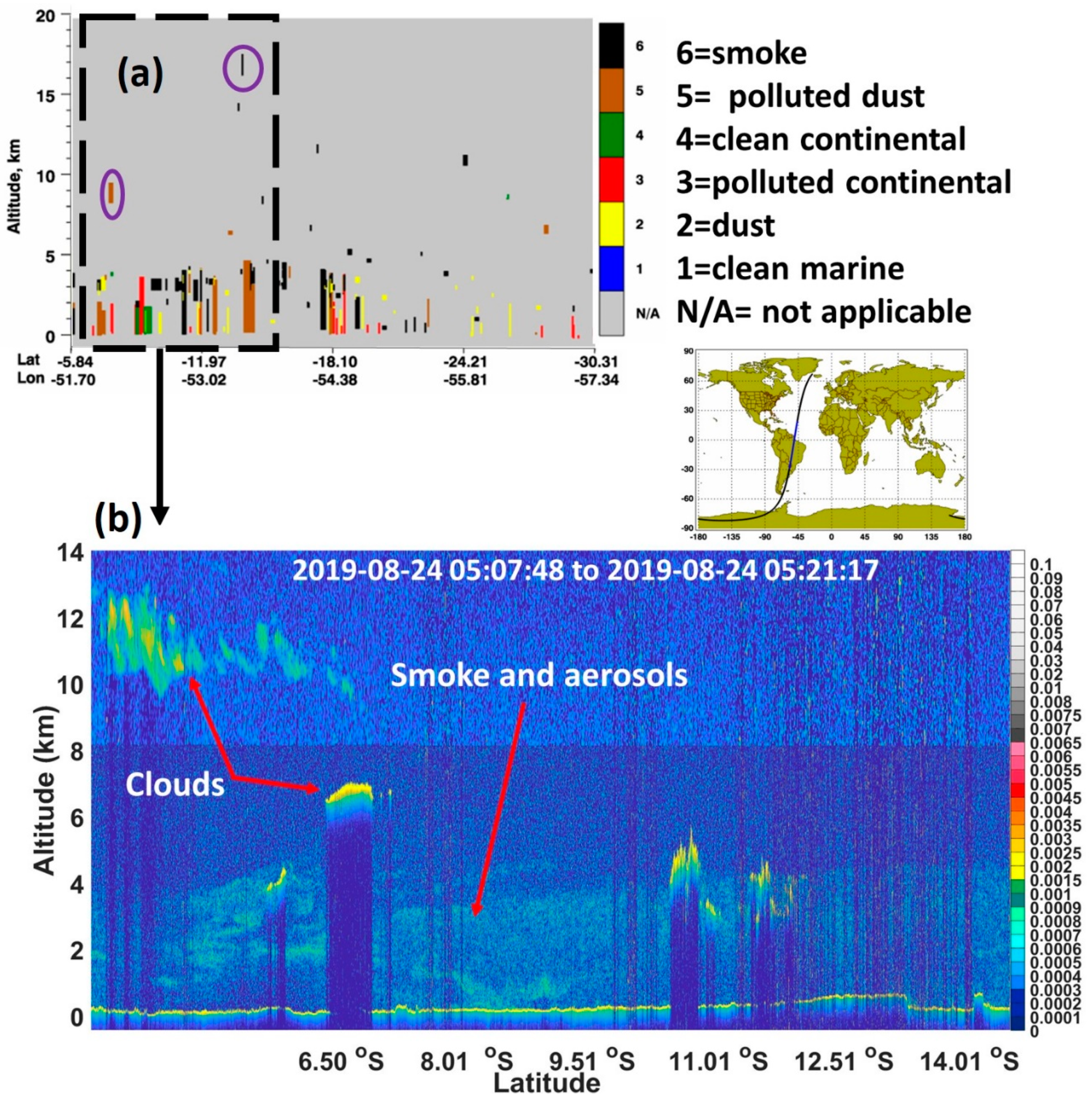
4.1.2. Brazil Fires (August 2019)
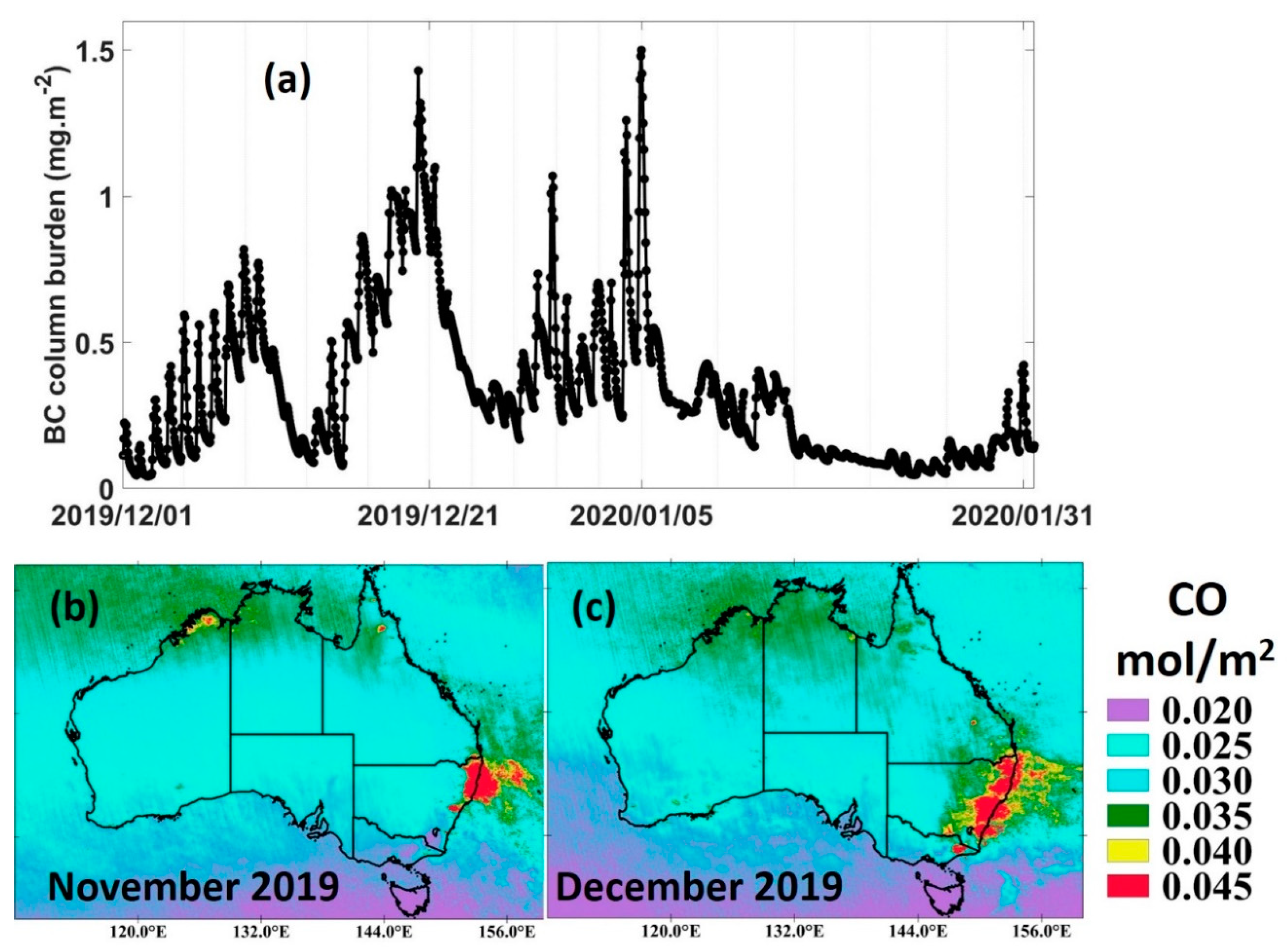
4.2. Similarities and Differences in the Fire Parameters over USA, Brazil, and Australia
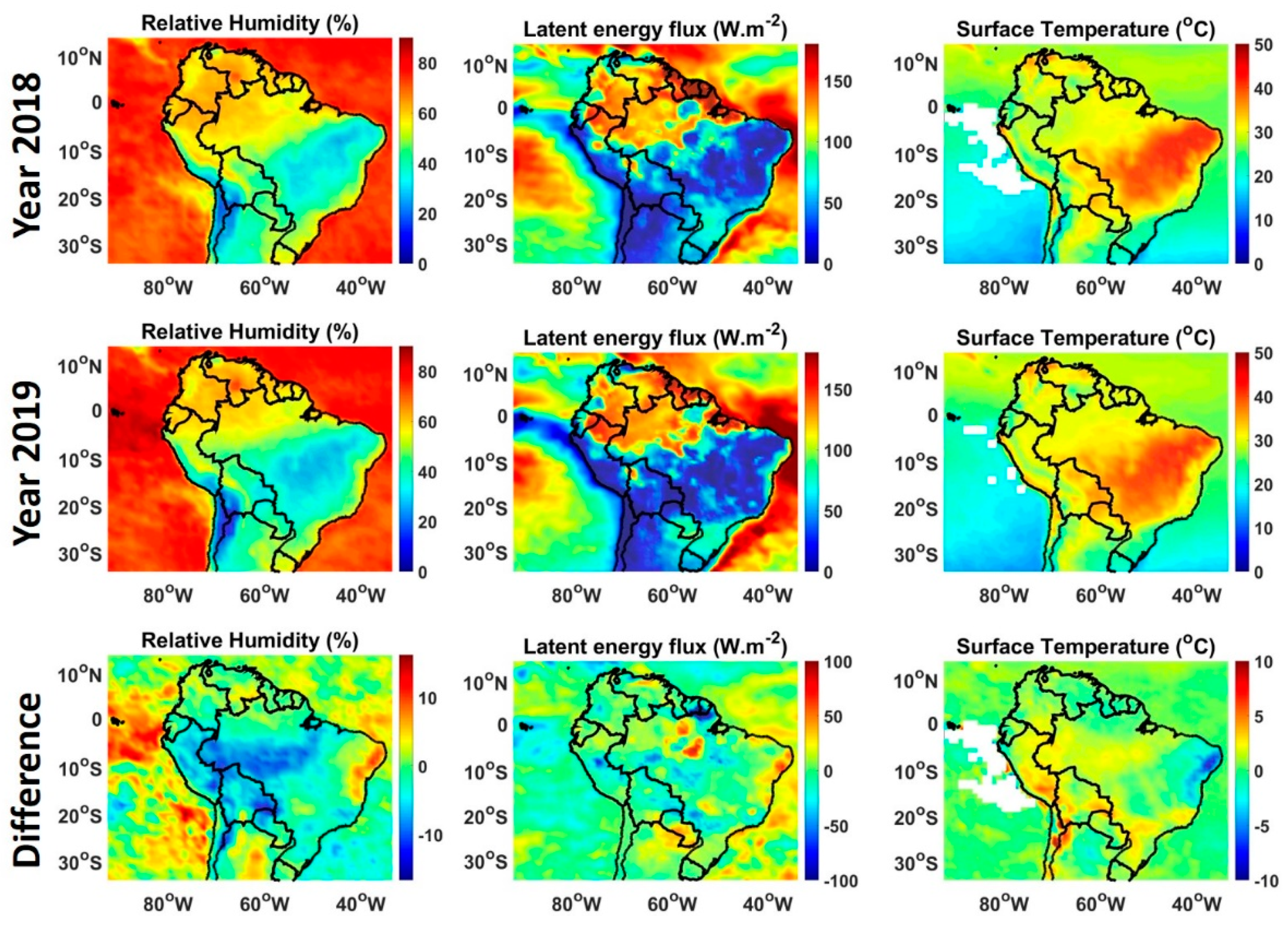
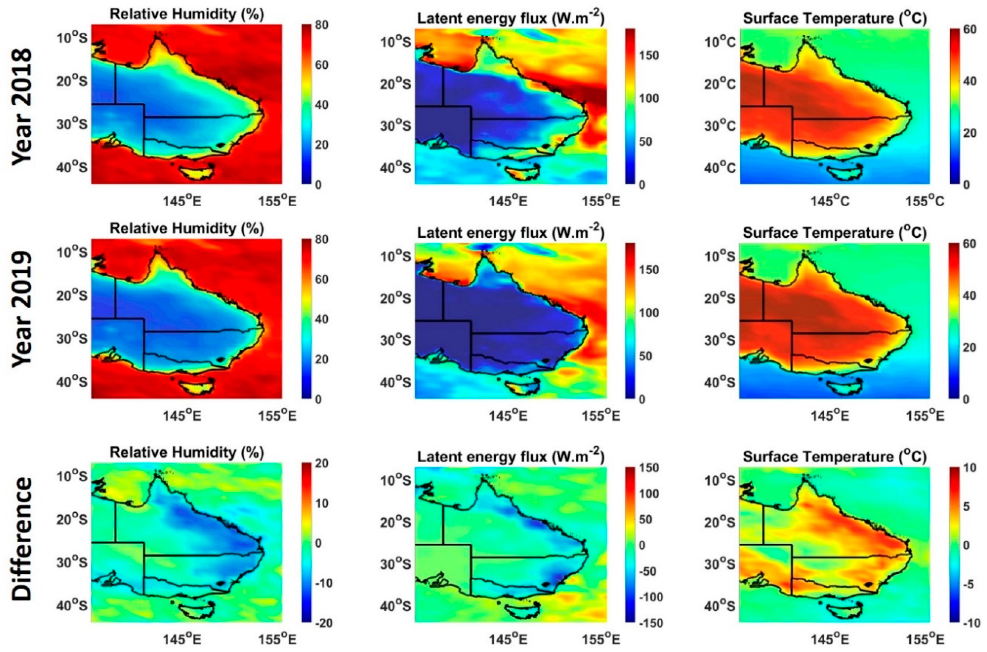
4.3. Analysis of the Meteorological Conditions during the Period of the Wildfires
5. Conclusions
Author Contributions
Funding
Acknowledgments
Conflicts of Interest
References
- Liu, J.C.; Wilson, A.; Mickley, L.J.; Dominici, F.; Dominici, F.; Ebisu, K.; Wang, Y.; Sulprizio, M.P.; Peng, R.D.; Yue, X.; et al. Wildfire-specific Fine Particulate Matter and Risk of Hospital Admissions in Urban and Rural Counties. Epidemiology 2017, 8, 77–85. [Google Scholar]
- Thomas, D.S.; Butry, D.T.; Gilbert, S.W.; Webb, D.; Fung, J. The Costs and Losses of Wildfires; Special Publication (NIST SP)—1215; NIST: Gaithersburg, MD, USA, 2018. [CrossRef]
- Harper, A.R.; Doerr, S.H.; Santin, C.; Froyd, C.A.; Sinnadurai, P. Prescribed fire and its impacts on ecosystem services in the UK. Sci. Total Environ. 2018, 624, 691–703. [Google Scholar] [PubMed] [Green Version]
- Shikwambana, L.; Ncipha, X.; Malahlela, O.E.; Mbatha, N.; Sivakumar, V. Characterisation of aerosol constituents from wildfires using satellites and model data: A case study in Knysna, South Africa. Int. J. Remote Sens. 2019, 40, 4743–4761. [Google Scholar]
- Hardy, C.C.; Hermann, S.M.; Mutch, R.E. The Wildland Fire Imperative. In Smoke Management Guide for Prescribed and Wildland Fire, 2001st ed.; Hardy, C.C., Ottmar, R.D., Peterson, J.L., Core, J.C., Seamon, P., Eds.; National Wildfire Coordination Group, National Interagency Fire Center: Boise, ID, USA, 2002; pp. 11–19. [Google Scholar]
- Finney, M.A.; McHugh, C.W.; Grenfell, I.C. Stand– and landscape–level effects of prescribed burning on two Arizona wildfires. Can. J. For. Res. 2005, 35, 1714–1722. [Google Scholar]
- Liu, Y.; Goodrick, S.; Heilman, W. Wildland fire emissions, carbon, and climate: Wildfire–climate interactions. Forest Ecol. Manag 2014, 317, 80–96. [Google Scholar]
- Voulgarakis, A.; Field, R.D. Fire Influences on Atmospheric Composition, Air Quality and Climate. Curr. Pollution Rep. 2015, 70, 70–81. [Google Scholar]
- Christian, T.J.; Kleiss, B.; Yokelson, R.J.; Crutzen, P.J.; Hao, W.M.; Saharjo, B.H.; Ward, D.E. Comprehensive laboratory measurements of biomass–burning emissions: 1. Emissions from Indonesian, African, and other fuels. J. Geophys. Res. 2003, 108, 4719. [Google Scholar]
- Lasslop, G.; Kloster, S. Impact of fuel variability on wildfire emission estimates. Atmos. Environ. 2015, 121, 93–102. [Google Scholar]
- Kasischke, E.S.; Bruhwiler, L.P. Emissions of carbon dioxide, carbon monoxide, and methane from boreal forest fires in 1998. J. Geophys. Res. 2003, 107, 8146. [Google Scholar]
- Lazaridis, M.; Latos, M.; Aleksandropoulou, V.Ø.; Papayannis, A.; Tørseth, K. Contribution of forest fire emissions to atmospheric pollution in Greece. Air Qual. Atmos. Health 2008, 1, 143–158. [Google Scholar]
- Minschwaner, K.; Manney, G.L.; Livesey, N.J.; Pumphrey, H.C.; Pickett, H.M.; Froidevaux, L.; Lambert, A.; Schwartz, M.J.; Bernath, P.F.; Walker, K.A.; et al. The photochemistry of carbon monoxide in the stratosphere and mesosphere evaluated from observations by the Microwave Limb Sounder on the Aura satellite. J. Geophys. Res. 2010, 115, D13303. [Google Scholar]
- Giglio, L.; Schroeder, W.; Justice, C.O. The collection 6 MODIS active fire detection algorithm and fire products. Remote Sens. Environ. 2016, 178, 31–41. [Google Scholar] [PubMed] [Green Version]
- Vadrevu, K.; Lasko, K. Intercomparison of MODIS AQUA and VIIRS I-Band Fires and Emissions in an Agricultural Landscape—Implications for Air Pollution Research. Remote Sens. 2018, 10, 978. [Google Scholar]
- Di Biase, V.; Laneve, G. Geostationary Sensor Based Forest Fire Detection and Monitoring: An Improved Version of the SFIDE Algorithm. Remote Sens. 2018, 10, 741. [Google Scholar]
- Labonne, M.; Breon, F.-M.; Chevallier, F. Injection height of biomass burning aerosols as seen from a spaceborne lidar. Geophys. Res.Lett. 2007, 34, L11806. [Google Scholar]
- Huang, H.; Roy, D.P.; Boschetti, L.; Zhang, H.K.; Yan, L.; Kumar, S.S.; Gomez-Dans, J.; Li, J. Separability Analysis of Sentinel-2A Multi-Spectral Instrument (MSI) Data for Burned Area Discrimination. Remote Sens. 2016, 8, 873. [Google Scholar]
- Shikwambana, L. Long-term observation of global black carbon, organic carbon and smoke using CALIPSO and MERRA-2 data. Remote Sens. Lett. 2019, 10, 373–380. [Google Scholar]
- Kganyago, M.; Shikwambana, L. Assessing Spatio-Temporal Variability of Wildfires and their Impact on Sub-Saharan Ecosystems and Air Quality Using Multisource Remotely Sensed Data and Trend Analysis. Sustainability 2019, 11, 6811. [Google Scholar]
- Lizundia-Loiola, J.; Pettinari, M.L.; Chuvieco, E. Temporal Anomalies in Burned Area Trends: Satellite Estimations of the Amazonian 2019 Fire Crisis. Remote Sens. 2020, 12, 151. [Google Scholar]
- BBC. Australia Fires: A Visual Guide to the Bushfire Crisis. Available online: https://www.bbc.com/news/world-australia-50951043 (accessed on 23 October 2020).
- Whiteside, P.G. Scorched Earth: How the Devastating Australia Fires Compare to Those in California and Brazil. Available online: https://news.sky.com/story/scorched-earth-how-the-australia-fires-compare-to-us-and-brazil-11904192 (accessed on 23 October 2020).
- Kganyago, M.; Shikwambana, L. Assessment of the Characteristics of Recent Major Wildfires in the USA, Australia and Brazil in 2018–2019 Using Multi-Source Satellite Products. Remote Sens. 2020, 12, 1803. [Google Scholar]
- Winker, D.M.; Vaughan, M.A.; Omar, A.; Hu, Y.; Powell, K.A.; Liu, Z.; Hunt, W.H.; Young, S.A. Overview of the CALIPSO Mission and CALIOP Data Processing Algorithms. J. Atmos. Ocean. Technol. 2009, 26, 2310–2323. [Google Scholar] [CrossRef]
- Hunt, W.H.; Winker, D.M.; Vaughan, M.A.; Powell, K.A.; Lucker, P.L.; Weimer, C. CALIPSO Lidar Description and Performance Assessment. J. Atmos. Ocean. Tech. 2009, 26, 1214–1228. [Google Scholar] [CrossRef]
- Peterson, D.A.; Campbell, J.R.; Hyer, E.J.; Fromm, M.D.; Kablick, G.P., III; Cossuth, J.H.; DeLand, M.T. Wildfire-driven thunderstorms cause a volcano-like stratospheric injection of smoke. NPJ Clim. Atmos. Sci. 2018, 1, 30. [Google Scholar] [CrossRef] [PubMed] [Green Version]
- Naeger, A.R.; Christopher, S.A.; Ferrare, R.; Liu, Z. A New Technique Using Infrared Satellite Measurements to Improve the Accuracy of the CALIPSO Cloud-Aerosol Discrimination Method. IEEE Trans Geosci Remote Sens. 2012, 51, 642–653. [Google Scholar] [CrossRef]
- Theys, N.; Hedelt, P.; De Smedt, I.; Lerot, C.; Yu, H.; Vlietinck, J.; Pedergnana, M.; Arellano, S.; Galle, B.; Fernandez, D.; et al. Global monitoring of volcanic SO2 degassing with unprecedented resolution from TROPOMI onboard Sentinel-5 Precursor. Sci. Rep. 2019, 9, 2643. [Google Scholar] [CrossRef]
- Rienecker, M.M.; Suarez, M.J.; Gelaro, R.; Todling, R.; Bacmeister, J.; Liu, E.; Bosilovich, M.G.; Schubert, S.D.; Takacs, L.; Kim, G.; et al. MERRA: NASA’s Modern-Era Retrospective Analysis for Research and Applications. J. Clim. 2011, 24, 3624–3648. [Google Scholar] [CrossRef]
- Gelaro, R.; McCarty, W.; Suárez, M.J.; Todling, R.; Molod, A.; Takacs, L.; Randles, C.A.; Darmenov, A.; Bosilovich, M.G.; Reichle, R.; et al. The Modern-Era Retrospective Analysis for Research and Applications, Version 2 (MERRA-2). J. Clim. 2017, 30, 5419–5454. [Google Scholar] [CrossRef]
- Buchard, V.; Randles, C.A.; da Silva, A.M.; Darmenov, A.; Colarco, P.R.; Govindaraju, R.; Ferrare, R.; Hair, J.; Beyersdorf, A.J.; Ziemba, L.D.; et al. The MERRA-2 Aerosol Reanalysis, 1980 Onward. Part II: Evaluation and Case Studies. J. Clim. 2017, 30, 6851–6872. [Google Scholar] [CrossRef]
- Morse, P.G.; Bates, J.C.; Miller, C.R.; Chahine, M.T.; O’Callaghan, F.; Aumann, H.H.; Karnik, A.R. Development and test of the Atmospheric Infrared Sounder (AIRS) for the NASA Earth Observing System (EOS). In Proceedings of the SPIE 3870, Sensors, Systems, and Next-Generation Satellites III, Florence, Italy, 28 December 1999. [Google Scholar] [CrossRef]
- Lambrigtsen, B.; Fetzer, E.; Fishbein, E.; Lee, S.-Y.; Pagano, T. AIRS—The Atmospheric Infrared Sounder. IEEE Trans. Geosci. Remote Sens. Symp. 2004, 2204–2207. [Google Scholar] [CrossRef]
- Val Martin, M.; Kahn, R.A.; Tosca, M.G. A Global Analysis of Wildfire Smoke Injection Heights Derived from Space-Based Multi-Angle Imaging. Remote Sens. 2018, 10, 1609. [Google Scholar] [CrossRef] [Green Version]
- Escobar, H. Amazon fires clearly linked to deforestation. Science 2019, 365, 853. [Google Scholar] [CrossRef] [PubMed]
- Formenti, P.; Andreae, M.O.; Lange, L.; Roberts, G.; Cafmeyer, J.; Rajta, I.; Maenhaut, W.; Holben, N.; Artaxo, P.; Lelieveld, J. Saharan dust in Brazil and Suriname during the Large-Scale Biosphere-Atmosphere Experiment in Amazonia (LBA)—Cooperative LBA Regional Experiment (CLAIRE) in March 1998. J. Geophys. Res. 2001, 106, 14919–14934. [Google Scholar] [CrossRef]
- Keith, D.A. A Compilation Map of Native Vegetation for NSW. National Parks & Wildlife Service. 2002. Available online: https://www.epa.nsw.gov.au/soe/soe2003/chapter6/map6.1.htm (accessed on 23 October 2020).
- Chen, J.; Li, C.; Ristovski, Z. A review of biomass burning: Emissions and impacts on air quality, health and climate in China. Sci. Total Environ. 2017, 579, 1000–1034. [Google Scholar] [CrossRef] [PubMed] [Green Version]
- Lu, Z.; Sokolik, I.N. The Impacts of Smoke Emitted from Boreal Forest Wildfires on the High Latitude Radiative Energy Budget—A Case Study of the 2002 Yakutsk Wildfires. Atmosphere 2018, 9, 410. [Google Scholar] [CrossRef] [Green Version]
- Kaufman, Y.J.; Koren, I.; Remer, L.A.; Rosenfeld, D.; Rudich, Y. The effect of smoke, dust, and pollution aerosol on shallow cloud development over the Atlantic Ocean. Proc. Natl. Acad. Sci. USA 2005, 102, 11207–11212. [Google Scholar] [CrossRef] [PubMed] [Green Version]
- Kleidon, A. Energy Balance. Encycl. Ecol. 2019, 50–63. [Google Scholar] [CrossRef]
- Moreira de Araújo, F.; Ferreira, L.G.; Arantes, A.E. Distribution Patterns of Burned Areas in the Brazilian Biomes: An Analysis Based on Satellite Data for the 2002–2010 Period. Remote Sens. 2012, 4, 1929–1946. [Google Scholar] [CrossRef] [Green Version]
- Mbatha, N.; Xulu, S. Time Series Analysis of MODIS-Derived NDVI for the Hluhluwe-Imfolozi Park, South Africa: Impact of Recent Intense Drought. Climate 2018, 6, 95. [Google Scholar] [CrossRef] [Green Version]
- Nolan, R.H.; Boer, M.M.; Collins, L.; Resco de Dios, V.; Clarke, H.; Jenkins, M.; Kenny, B.; Bradstock, R.A. Causes and consequences of eastern Australia’s 2019-20 season of mega-fires. Glob. Change Biol. 2020, 26, 1039–1041. [Google Scholar] [CrossRef] [Green Version]
- Bencherif, H.; Bègue, N.; Kirsch Pinheiro, D.; du Preez, D.J.; Cadet, J.-M.; da Silva Lopes, F.J.; Shikwambana, L.; Landulfo, E.; Vescovini, T.; Labuschagne, C.; et al. Investigating the Long-Range Transport of Aerosol Plumes Following the Amazon Fires (August 2019): A Multi-Instrumental Approach from Ground-Based and Satellite Observations. Remote Sens. 2020, 12, 3846. [Google Scholar] [CrossRef]
- Giulia, U.; Gianluca, R.; Mat, S. Experimental evidence of the multiple microclimatic impacts of bushfires in affected urban areas: The case of Sydney during the 2019/2020 Australian season. Environ. Res. Commun. 2020, 2, 065005. [Google Scholar]
- Mueller, S.; Tarnay, L.; O’Neill, S.; Raffuse, S. Apportioning Smoke Impacts of 2018 Wildfires on Eastern Sierra Nevada Sites. Atmosphere 2020, 11, 970. [Google Scholar] [CrossRef]


| Parameter | USA | Brazil | Australia |
|---|---|---|---|
| BC column burden (mg/m2) | 0.6 | 0.5 | 1.5 |
| Smoke + aerosol height (km) | 4 | 4 | 6 |
| CO (mol/m2) | 0.05 | 0.05 | 0.045 |
| * Burnt area (km2) | 800 | 4000 | 2800 |
| * Temperature (during the fire) (°C) | ~42 | ~32 | ~42 |
| * Relative humidity (during the fire) (%) | ~30 | ~50 | ~40 |
| * Average wind speed (m/s) | ~6 | ~6 | ~4 |
| * Number of Active Fires | 1098 | 14,128 | 5613 |
| * Mean Fire Radiation Power (MW) | 762.07 | 356.77 | 494.37 |
Publisher’s Note: MDPI stays neutral with regard to jurisdictional claims in published maps and institutional affiliations. |
© 2020 by the authors. Licensee MDPI, Basel, Switzerland. This article is an open access article distributed under the terms and conditions of the Creative Commons Attribution (CC BY) license (http://creativecommons.org/licenses/by/4.0/).
Share and Cite
Shikwambana, L.; Kganyago, M. Observations of Emissions and the Influence of Meteorological Conditions during Wildfires: A Case Study in the USA, Brazil, and Australia during the 2018/19 Period. Atmosphere 2021, 12, 11. https://doi.org/10.3390/atmos12010011
Shikwambana L, Kganyago M. Observations of Emissions and the Influence of Meteorological Conditions during Wildfires: A Case Study in the USA, Brazil, and Australia during the 2018/19 Period. Atmosphere. 2021; 12(1):11. https://doi.org/10.3390/atmos12010011
Chicago/Turabian StyleShikwambana, Lerato, and Mahlatse Kganyago. 2021. "Observations of Emissions and the Influence of Meteorological Conditions during Wildfires: A Case Study in the USA, Brazil, and Australia during the 2018/19 Period" Atmosphere 12, no. 1: 11. https://doi.org/10.3390/atmos12010011