Reversibility of the Hydrological Response in East Asia from CO₂-Derived Climate Change Based on CMIP6 Simulation

Abstract

Understanding the response of the Earth system to CO₂ removal (CDR) is crucial because the possibility of irreversibility exists. Therefore, the Carbon Dioxide Removal Model Inter-comparison Project (CDRMIP) for the protocol experiment in the Coupled Model Inter-comparison Project Phase 6 (CMIP6) has been developed. Our analysis focuses on the regional response in the hydrological cycle, especially in East Asia (EA). The peak temperature changes in EA (5.9 K) and the Korean peninsula (KO) (6.1 K) are larger than the global mean surface air temperature (GSAT) response. The precipitation changes are approximately 9.4% (EA) and 23.2% (KO) at the phase change time (130–150 years); however, the largest increase is approximately 16.6% (EA) and 36.5% (KO) in the ramp-down period (150–160 years). In addition, the differences are below 5 mm/day and 1 day for the precipitation intensity indices (Rx1day and Rx5day) and frequency indices (R95 and R99), respectively. Furthermore, the monsoon rainband of the ramp-down period moves northward as the earlier onset with high confidence compared to the ramp-up period; however, it does not move north to the KO region. The results suggest that reducing CO₂ moves the rainband southward. However, a detailed interpretation in terms of the mechanism needs to be carried out in further research.

1. Introduction

The concentration of carbon dioxide (CO₂), an important greenhouse gas (GHG), has increased over 400 ppm in the atmosphere as a result of anthropogenic activities [1]. This CO₂ increase results in global warming [2], and recent trends have shown that the atmospheric CO₂ concentration will continue to increase [3]. Climate tipping points have become the focus areas of research in the assessment of the impacts associated with climate change [4,5,6,7]. The IPCC [8] reports that a climate tipping point leads to irreversible and significant additional global warming, which is more than 2 °C above the pre-industrial (PI) temperature level. Therefore, the Paris Agreement of the 21st session of the Conference of Parties (COP21) on climate change [9] has established the goal of limiting anthropogenic warming to below 2 °C of the PI temperature level. To limit the global warming by 1.5 °C, CO₂ emissions will have to be reduced quickly enough to reach negative emission levels [10].

Thus, mitigation scenarios and expected future projections are needed to reduce future climate change risk [11,12]. Following this, several scenarios such as “overshoot” and “peak and decline” scenarios (decreasing after atmospheric GHG exceeding a particular target) have been considered to characterize the mitigation effect and irreversible change [13]. In addition, modeling studies of mitigation (e.g., carbon dioxide removal (CDR)) with Earth system Models of Intermediate Complexity (EMIC) simulations have been performed [14,15,16]. These idealized simulations of the Earth system model suggest that CDR can limit or reverse warming and can change many other climate variables [17,18,19,20]. The results of these studies are not directly comparable because different mitigation scenarios and experimental designs were considered. Therefore, there is an urgent need to understand the response of the Earth system to CDR as it is increasingly being used in mitigation/adaptation policy and economic discussions. CDRMIP was first developed to advance the understanding of CDR [21] for the protocol experiment in the CMIP6. The CDRMIP experiments are prioritized based on a tier system, and an idealized Tier 1 experiment (C1 experiment) is used in this study. The C1 experiment is designed to investigate CDR-induced climate reversibility through a simple procedure (details in Section 2).

Previous studies have shown that the changes in surface air temperature due to CO₂ emissions can be reversed with negative emissions [17,18,22]. However, the changes in precipitation and oceanic properties show a delay in their response to CO₂ reduction [18,23,24]. Overall, CDR modeling studies on inducing climate reversibility have suggested that many properties are reversible, and several properties (related to precipitation and oceanic variables) show non-linear responses at the global scale [17,19,20,25]. Therefore, we evaluate the reversibility of general performance of CMIP6 models, conducting and updated analysis of previous studies. Herein, we further investigate the response of hydrological cycle to CO₂ changes with extreme indices and the characteristics of East Asia Summer Monsoon (EASM) focusing on EA and Korea peninsula regions. There are two reasons for this approach. First, the climate reversibility of extreme indices plays an important role in reducing climate change risk and implementing mitigation and adaptation plans; therefore, we need a better understanding of the CDR response of the Earth system. Second, there is a lack of regional-scale studies on seasonal phenomena such as the EASM. Understanding the reversibility of the EASM has significant economic implications for the EA region, because it affects agricultural and water resource management decisions. This approach provides new insights into climate reversibility at the regional scale. In addition, this result will benefit policymakers and environmental planners dealing with climate change effects.

2. Experiment and Methodology

The C1 experiment of the Carbon Dioxide Removal Model Inter-comparison Project (CDRMIP) [21] is used in this study. Following the control (PI) period starting from the conditions at 1850 (atmospheric CO₂ concentration of 284.7 ppm), the prescribed atmospheric CO₂ concentration is increased by 1% per year. A restart of the simulation must be generated when the atmospheric CO₂ concentration reaches four times (1139 ppm) that of PI and a decrease in concentration by 1% per year for the next 140 years is followed to reach the initial CO₂ level. The CO₂ concentration should be held at 284.7 ppm for as long as possible, but we employ 60 years (Tier 1 experiment). We have performed this C1 experiment with Korea Meteorological Administration Advanced Community Earth-System model (K-ACE) [26,27] and the UK Earth System Model (UKESM1) [28]. In addition, other CMIP6 data are available through the Earth System Grid Federation, which is one of the most complex big data systems [29]. Overall, a total of 6 CMIP6 models are used (K-ACE, UKESM1-0-LL, Australian Community Climate and Earth System Simulator–Earth System Model (ACCESS-ESM1-5), Canadian Earth System Model version 5 (CanESM5), Community Earth System Model version 2 (CESM2), and Model for Interdisciplinary Research on Climate, Earth System version 2 for Long-term simulations (MIROC-ES2L)).

Our analysis is conducted at the global and regional scales over East Asia (EA) (110–140° E, 20–50° N) and the Korean peninsula (KO; 124–132° E, 32–43° N). The variables used in this study include monthly and daily surface air temperature and precipitation. Furthermore, extreme precipitation over the land of global, EA, and KO are analyzed with ETCCDI (Expert Team on Climate Change Detection and Indices) recommended by the World Meteorological Organization (WMO). The four extreme precipitation indices (R×1day and R×5day: maximum consecutive 1 day and 5 day precipitation amount, R95 and R99: annual count of heavy precipitation days when daily precipitation exceeds the 95th and 99th percentile) are selected. These can be classified into precipitation intensity and frequency, respectively. Additionally, for analyzing the EASM reversibility, we use the Wang and Linho [30] method, which calculates the rainy and dry seasons to represent monsoon characteristics (onset, duration, withdrawal, and amount) over EA and KO. The onset of rainy season is defined as the day when the difference between the pentad mean precipitation and monthly mean in January is more than 5 mm day⁻¹. Withdrawal is defined as the day after the onset, in which the difference is less than 5 mm day⁻¹. The monsoon duration is defined as the difference between withdrawal and onset days. The difference between the mean for the first 20 years (P1 period; 0–19 years) and that for the last 20 years (P2 period; 261–280 years) determines the reversibility of the climate indices.

3. Results

3.1. Changes in Temperature and Precipitation

Figure 1a shows the global mean surface air temperature (GSAT) response over the entire simulation period relative to the average PI level. The GSAT increases with rising atmospheric CO₂ and reaches a peak of approximately 5.4 K (130–150 years) above the PI level. As the CO₂ concentration decreases, the GSAT change also quickly decreases. However, the rate of decrease is −0.03 K year⁻¹, which is slower than the increasing rate (−0.04 K year⁻¹). When the CO₂ concentration returns to the PI level, the GSAT change value remains approximately 1.5 K above its initial value. This result is similar to those of previous studies [17,20,31]. Figure 1b shows the latitudinal temperature change rates (K). Temperature changes are similarly reversed within the timescale of CO₂ reversal and all the latitudes remain at a warming temperature of more than the PI level after 280 years. In particular, at the northern higher latitudes, the largest percentage change occurs at above 60° N. In mid-latitudes (30–60° N), the temperature changes are larger than other latitudes (except for the northern high latitude). This indicates that the peak temperature changes of EA and KO are larger than the GSAT response (Figure 1a). Therefore, the increasing and decreasing rate of temperature in EA and KO are higher than those in GSAT (Figure 1a). The peak temperature changes (130–150 years) of EA and KO are 5.9 K and 6.1 K, respectively. In addition, the temperature changes remain at 0.91 K (EA) and 0.84 K (KO) in the P2 period, and these values are smaller than the GSAT response. This demonstrates that even if the atmospheric CO₂ reduces, the reversibility of global and regional climate is different.

Figure 2a shows the global mean precipitation response to the ramping up and down of CO₂ concentration. An increasing amount of global precipitation occurs at approximately 9% with the simulated CO₂ increase, and the largest increase is approximately 10% at 161 years. This means that the maximum increase in the ramp-up period is 9% and even if CO₂ decreases, precipitation increases further by 1% due to inertia effects in the previous phase. This is consistent with previous studies [32,33]. It is interesting to note the transient acceleration of the global hydrological cycle shown by reversibility studies [17,32,33]. In addition, similar phenomena occur in EA and KO. The largest increase is approximately 16.6% (EA) and 36.5% (KO) in the ramp-down period (150–160 years). After the peak, the precipitation quickly decreases in response to CO₂ reduction. Unlike the temperature response that decreases following CO₂ reduction, the global mean precipitation increases slightly due to the fast cooling atmosphere and slow cooling oceans before gradually decreasing. In addition, the precipitation change (P2 minus P1) does not fully return to the PI levels of approximately 4.1%, 2.3%, and 0.1% in global, EA, and KO regions, respectively. The variability of the mean change in precipitation in EAs is similar to that of global precipitation. However, the KO region locates the boundary of the main monsoon band, and periodic northward expanded flows are the main source of summer precipitation. Therefore, the mean change in precipitation in the KO region is much larger than those in the global and EA regions (Figure 2a).

Figure 2b shows the latitudinal precipitation change rates (%). The precipitation increases in the high northern latitudes (above 60° N), around 20° N latitudes and the equator (EQ), during the ramp-up period and also remained high during the ramp-down period. The precipitation around 20° N and EQ bands shows a large amount of remaining precipitation over the East Pacific region and the South Pacific Convergence Zone within the 280 years of CO₂ changes (not shown). This precipitation response is similar to those reported by previous studies [17,32], which report that the change in global mean precipitation is dominated by changes in the ocean rather than land. However, the mid-latitude regions (including EA and KO) seem to be reversible, while the equatorial tropical and northern subtropical regions remain at 37% and 20% of precipitation with changing CO₂, respectively (Figure 2b). These results demonstrate that the local reversibility of climate varies with spatial differences; therefore, regional analysis is important for understanding the CDR reversibility.

3.2. Hydrological Climate Extreme Indices

Figure 3 shows the differences in four hydrological extreme indices (intensity indices (R×1day and R×5day) and frequency indices (R95 and R99)) between the P2 and P1 period. Spatially, the differences show similar distributions in the EA region (Figure 3), which is similar with global distribution (not shown). There are strong wet signals over Southern China and Japan and a weak dry signal in the northern Korea peninsula. These patterns suggest spatial differences in the timescale of reversibility after the CO₂ concentration ramp-down. However, the regional averaged values of extreme indices are similar between the P2 and P1 periods (Figure 4). The differences are below 5 mm for precipitation intensity indices (R×1day and R×5day) and below 1 day for frequency indices (R95 and R99), respectively. In the precipitation intensity indices, a simulated range of CMIP6 models for the P2 period is slightly higher than that for the P1 period in both the global and EA regions. However, the medians of the two periods are similar. The frequency indices of the P2 period are larger than those of the P1 period in the global and EA regions. In particular, the spread range of the frequency indices is widely distributed above median. In the KO region, four hydrological indices in the P2 period are smaller than those in the P1 period, which is a different trend from that of the global and EA region. This can be attributed to the uncertainty in the model, because the KO region is narrow. Although it is an analysis of the extreme indices over land, the precipitation intensity may return to the previous state following the CO₂ reduction, but it may not return in precipitation frequency.

3.3. Characteristics of EASM

Before analyzing the C1 experiment, the performance of simulated precipitation (June–August) in EA using the result (1995–2014) of CMIP6 historical simulation shows a pattern correlation coefficient of approximately 0.8 (not shown herein). Furthermore, the simulated main rainband shows reasonable performance; therefore, the analysis results of this section do not get affected by the bias of each model.

The time–latitude Hovmöller diagram shows the seasonal monsoon rainband over the EA region (Figure 5). This cross-section analysis is a useful tool to assess the inter-seasonal variation in the EASM and associated monsoon characteristics (onset and withdrawal time) [34]. In the spring, the rainband occurs in association with around 30° N latitude, although the precipitation amount is smaller than that in the summer (Figure 5a,b). Following the enhancement of the frontal system associated with moisture support, the rainband shows seasonal movement northward. Similarly, several previous studies report that the EASM propagates northward, beginning in mid-May in the South China Sea and in late June in Korea [30,35,36,37,38,39,40]. The latitudinal rainband around 30° N in the P2 period appears more northward than that in the P1 period (Figure 5c). By contrast, in the summer, dry and wet signals appear around 40° N and south of 30° N, respectively. The larger precipitation amount occurs south of 30° N due to the simulated rainband location shifted southward. Following this, the dry signal directly appears after summer, which means that the rainband is located south of 20° N. These results show that the monsoon rainband is shifted southward and seasonal severe droughts may appear in the KO region.

The rainband of EASM and seasonal evolution varies considerably with latitude [30]. Thus, we define EA and KO regions with three parts to investigate monsoon evolution by latitudes (Figure 6a). Latitudinally, the EA1, EA2, and EA3 domains cover 20–30° N, 30–40° N, and 40–50° N, respectively. Furthermore, the KO1, KO2, and KO3 domains cover 32–35° N, 35–39° N, and 39–43° N, respectively.

Table 1. The difference in East Asia Summer Monsoon (EASM) characteristics between P2 and P1 periods in terms of onset, withdrawal, duration, mean, and maximum precipitation amount.

Region	Onset	Withdrawal	Duration	Amount (mm/day)	Max (mm/day)
East Asia	−0.4	0.2	0.6	16.7	0.7
EA1	−0.5	−0.1	0.6	24.1	0.7
EA2	−0.3	0.3	0.6 **	13.2	0.8
EA3	−0.2	0.2	0.4	9.6	0.3
Korea	−0.6 **	−0.02	0.6 **	11.6	0.3
KO1	−1.6 **	0.2	1.8 **	38.3	3.8
KO2	−0.4	−0.4	0.05	3.0	−1.8
KO3	−0.3	−0.1	0.2	0.3	−0.6

Notes: ** denotes statistical significance at 90% level.

shows the simulated differences between the P2 and P1 period in the onset, withdrawal, duration, and precipitation amount. For the P2 period in EA, the earlier onset and delayed withdrawal (except EA1) lead long duration; therefore, the total and maximum amount of precipitation is larger than that in the P1 period. All the three sub-regions (EA1, EA2, and EA3) show similar trends. However, the total precipitation amount (24.1 mm/day) of EA1 (the most southern region) is significantly larger than those in the other two regions (Figure 6b). Considering this, the duration of EA2 shows a high confidence (p < 0.1). The EA2 includes KO, and the onset and duration of KO show a high confidence. This means that the onset pentad is major component of the duration of the P2 period. In particular, the duration of KO1 is lengthened by 1.8 pentads due to the early onset (1.6 pentads) of the monsoon season. This leads to a larger precipitation amount (total and maximum value) of KO1 in the P2 period than that in the P1 period. Unlike the KO1 region, KO2, and KO3 have very little difference between the P2 and P1 periods, suggesting that the monsoon rainband is shifted south of KO1, and this tendency appears in Figure 6b.

Overall, Figure 5 and Figure 6 and Table 1 show that the monsoon rainband in the P2 period is skewed to south of 30° N compared to the P1 period. The monsoon rainband moves northward in the spring as the earlier onset with high confidence, but it does not move north to the Korea peninsula. This result indicates that reducing CO₂ leads to the southward movement of the monsoon rainband. Furthermore, this leads to a reduction in precipitation in the Korea peninsula due to weaker northwestern pacific anticyclone and weaker northward flow in 850 hPa (not shown). A more detailed description of this mechanism requires further study. The climate reversibility of EASM provides a scientific basis for the establishment of adaptation policy to climate change. This study suggests that understanding the need for the assessment of regional changes may be necessary for the assessment of full reversibility.

4. Summary and Conclusion

This study systematically investigated the reversibility of CO₂-induced climate change using the CDRMIP protocol for the C1 experiment. The CO₂ concentration increased by 1%/year until 1139 ppm was reached (four times the PI level and for 140 years), whereas CO₂ reversed by 1%/year for 140 years to return to the PI level. Previous studies have shown the global mean changes for several climate components with the path dependency of CO₂ concentration changes. Considering this, we evaluate the reversibility of the general performance of CMIP6 models. Herein, we further investigate the response of the hydrological cycle to CO₂ changes with extreme indices and EASM characteristics focusing on EA and KO. The results are summarized as follows.

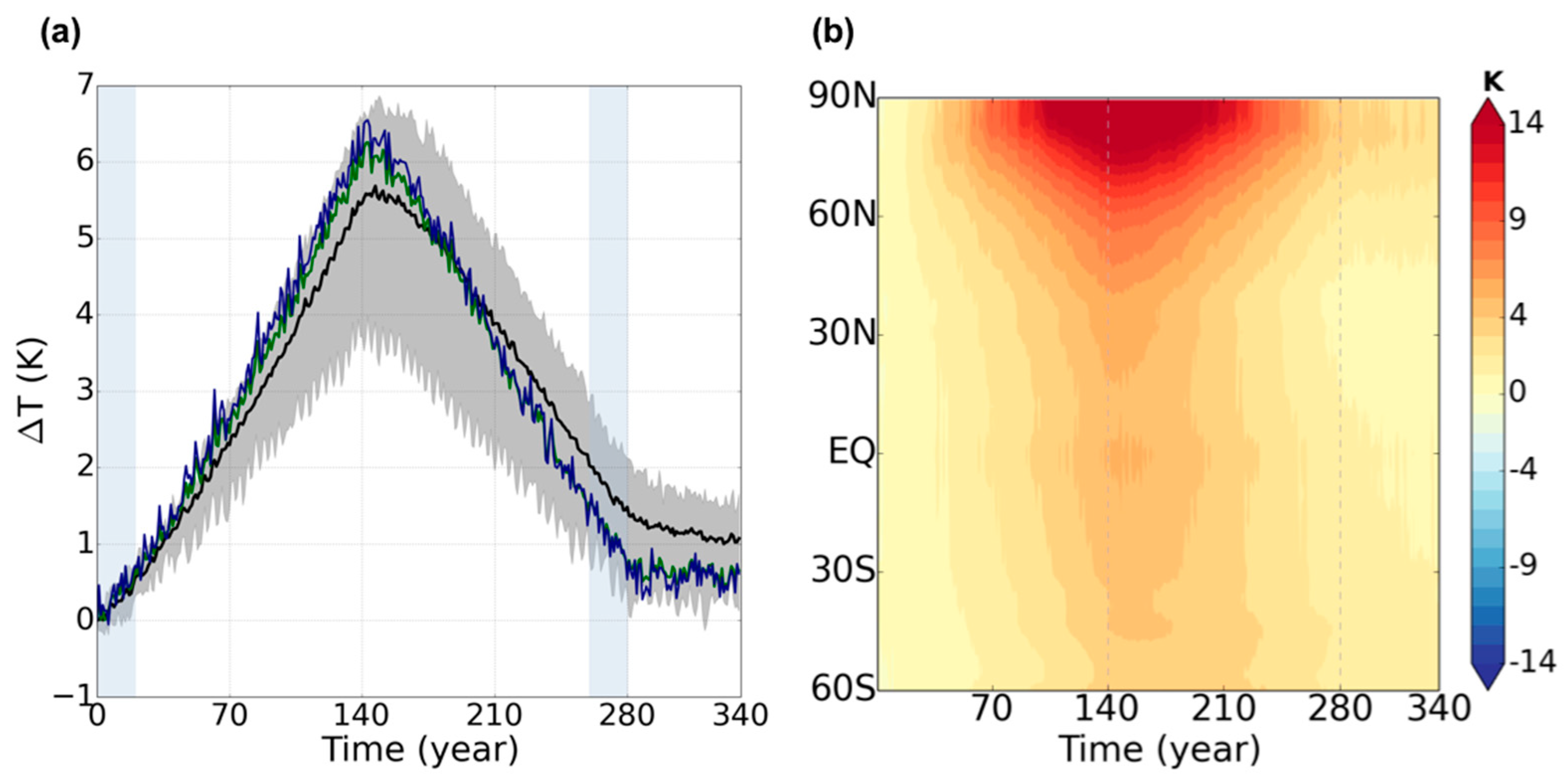
• The GSAT increases with increasing atmospheric CO₂ and reaches the peak value of 5.4 K above the PI level (130–150 years). The peak temperature changes in EA (5.9 K) and KO (6.1 K) are larger than those in the GSAT. In addition, EA and KO show higher rates of temperature increase and decrease than those shown by the GSAT. The temperature changes remain at 0.91 K (EA) and 0.84 K (KO) in the P2 period, and this value is smaller than the global value (approximately 1.5 K). However, this demonstrates that even if the CO₂ concentration is reduced, local climate may or may not return.
• The increasing amount is approximately 9.4% (EA) and 23.2% (KO) at the phase change time (averaged for 130–150 years); however, the largest increase is approximately 16.6% (EA) and 36.5% (KO) in the ramp-down period (150–160 years). After the peak, the precipitation quickly decreases in response to the CO₂ reduction. Unlike the temperature response that decreases following CO₂ reduction, the global mean precipitation increases slightly due to the fast cooling atmosphere and slow cooling oceans before gradually decreasing. These results demonstrate that the local reversibility of climate varies with spatial differences.
• The differences in the four hydrological extreme indices (between the P2 and P1 periods) have similar spatial distributions in EA. There are strong wet signals over Southern China and Japan and a weak dry signal over the northern Korea peninsula. The differences are below 5 mm/day and 1 day for precipitation intensity indices (R×1day and R×5day) and frequency indices (R95 and R99), respectively.
• We investigate the seasonal transition of EASM precipitation through a time–latitude diagram. The larger precipitation amount south of 30° N is related to the larger rainfall over South China with the southward movement of the monsoon rainband. The monsoon rainband of the P2 period moves northward as the earlier onset with high confidence compared to the P1 period, but it does not move north to the KO region. This analysis may indicate that a reduction in CO₂ leads to the southward movement of the monsoon rainband and reduced precipitation in the Korea peninsula. However, a more detailed description mechanism needs to be carried out in further research.

The proposed study investigates climate variables, hydrological extreme indices, and EASM characteristics at the global and regional (local) scales. These results suggest spatial differences in the timescale of the reversibility after the CO₂ concentration ramp-down. A better understanding of regional climate reversibility will help with implementing mitigation and adaptation plans. Our study provides new insights into the hydrological reversibility of EA and KO. In particular, the climate reversibility of the EASM characteristics provides a scientific basis for the establishment of policy initiatives for the adaptation to climate change. This study suggests that understanding the need for assessment of regional changes may necessary for the assessment of full reversibility.

References

1. Quéré, C.; Andrew, R.M.; Friedlingstein, P.; Sitch, S.; Pongratz, J.; Manning, A.C.; Korsbakken, J.I.; Peters, G.P.; Canadell, J.G.; Jackson, R.B. Global carbon budget 2017. Earth Syst. Sci. Data 2018, 10, 405–448. [Google Scholar] [CrossRef] [Green Version]
2. Stocker, T.F.; Qin, D.; Plattner, G.-K.; Alexander, L.V.; Allen, S.K.; Bindoff, N.L.; Bréon, F.-M.; Church, J.A.; Cubasch, U.; Emori, S. Technical summary. In Climate Change 2013: The Physical Science Basis. Contribution of Working Group I to the Fifth Assessment Report of the Intergovernmental Panel on Climate Change; Cambridge University Press: Cambridge, UK, 2013; pp. 33–115. [Google Scholar]
3. Peters, G.P.; Andrew, R.M.; Boden, T.; Canadell, J.G.; Ciais, P.; Le Quéré, C.; Marland, G.; Raupach, M.R.; Wilson, C. The challenge to keep global warming below 2 C. Nat. Clim. Chang. 2013, 3, 4–6. [Google Scholar] [CrossRef]
4. Cai, Y.; Lenton, T.M.; Lontzek, T.S. Risk of multiple climate tipping points should trigger a rapid reduction in CO2 emissions. Nat. Clim. Chang. 2016, 6, 520–525. [Google Scholar] [CrossRef] [Green Version]
5. Kriegler, E.; Hall, J.W.; Held, H.; Dawson, R.; Schellnhuber, H.J. Imprecise probability assessment of tipping points in the climate system. Proc. Natl. Acad. Sci. USA 2009, 106, 5041–5046. [Google Scholar] [CrossRef] [PubMed] [Green Version]
6. Steffen, W.; Rockström, J.; Richardson, K.; Lenton, T.M.; Folke, C.; Liverman, D.; Summerhayes, C.P.; Barnosky, A.D.; Cornell, S.E.; Crucifix, M. Trajectories of the Earth System in the Anthropocene. Proc. Natl. Acad. Sci. USA 2018, 115, 8252–8259. [Google Scholar] [CrossRef] [PubMed] [Green Version]
7. Lenton, A.; Matear, R.J.; Keller, D.P.; Scott, V.; Vaughan, N. Assessing carbon dioxide removal through global and regional ocean alkalization under high and low emission pathways. Earth Syst. Dyn. 2018, 9, 339–357. [Google Scholar] [CrossRef] [Green Version]
8. Field, C.B.; Barros, V.R.; Mach, K.J.; Mastrandrea, M.D.; van Aalst, M.; Adger, W.N.; Arent, D.J.; Barnett, J.; Betts, R.; Bilir, T.E. Technical Summary Climate Change 2014: Impacts, Adaptation, and Vulnerability. Part A: Global and Sectoral Aspects. Contribution of Working Group II to the Fifth Assessment Report of the Intergovernmental Panel on Climate Change; Field, C.B., Barros, V.R., Dokken, D.J., Eds.; Cambridge University Press: Cambridge, UK; New York, NY, USA, 2014. [Google Scholar]
9. UNFCCC. Paris Agreement of the 21st Session of the Conference of Parties on Climate Change; UNFCCC: Rio de Janeiro, Brazil, 2016. [Google Scholar]
10. Kriegler, E.; Luderer, G.; Bauer, N.; Baumstark, L.; Fujimori, S.; Popp, A.; Rogelj, J.; Strefler, J.; Van Vuuren, D.P. Pathways limiting warming to 1.5 °C: A tale of turning around in no time? Philos. Trans. R. Soc. A Math. Phys. Eng. Sci. 2018, 376, 20160457. [Google Scholar] [CrossRef] [Green Version]
11. Mignone, B.K.; Socolow, R.H.; Sarmiento, J.L.; Oppenheimer, M. Atmospheric stabilization and the timing of carbon mitigation. Clim. Chang. 2008, 88, 251–265. [Google Scholar] [CrossRef]
12. Rogelj, J.; Hare, W.; Lowe, J.; Van Vuuren, D.P.; Riahi, K.; Matthews, B.; Hanaoka, T.; Jiang, K.; Meinshausen, M. Emission pathways consistent with a 2 °C global temperature limit. Nat. Clim. Chang. 2011, 1, 413–418. [Google Scholar] [CrossRef]
13. Huntingford, C.; Lowe, J. “Overshoot” scenarios and climate change. Science 2007, 316, 829. [Google Scholar] [CrossRef]
14. Mikolajewicz, U.; Gröger, M.; Maier-Reimer, E.; Schurgers, G.; Vizcaíno, M.; Winguth, A.M.E. Long-term effects of anthropogenic CO2 emissions simulated with a complex earth system model. Clim. Dyn. 2007, 28, 599–633. [Google Scholar] [CrossRef]
15. Solomon, S.; Plattner, G.-K.; Knutti, R.; Friedlingstein, P. Irreversible climate change due to carbon dioxide emissions. Proc. Natl. Acad. Sci. USA 2009, 106, 1704–1709. [Google Scholar] [CrossRef] [PubMed] [Green Version]
16. Zickfeld, K.; Eby, M.; Weaver, A.J.; Alexander, K.; Crespin, E.; Edwards, N.R.; Eliseev, A.V.; Feulner, G.; Fichefet, T.; Forest, C.E. Long-term climate change commitment and reversibility: An EMIC intercomparison. J. Clim. 2013, 26, 5782–5809. [Google Scholar] [CrossRef]
17. Boucher, O.; Halloran, P.R.; Burke, E.J.; Doutriaux-Boucher, M.; Jones, C.D.; Lowe, J.; Ringer, M.A.; Robertson, E.; Wu, P. Reversibility in an Earth System model in response to CO2 concentration changes. Environ. Res. Lett. 2012, 7, 24013. [Google Scholar] [CrossRef]
18. Tokarska, K.B.; Zickfeld, K. The effectiveness of net negative carbon dioxide emissions in reversing anthropogenic climate change. Environ. Res. Lett. 2015, 10, 94013. [Google Scholar] [CrossRef] [Green Version]
19. Wu, P.; Ridley, J.; Pardaens, A.; Levine, R.; Lowe, J. The reversibility of CO2 induced climate change. Clim. Dyn. 2015, 45, 745–754. [Google Scholar] [CrossRef]
20. Zickfeld, K.; MacDougall, A.H.; Matthews, H.D. On the proportionality between global temperature change and cumulative CO2 emissions during periods of net negative CO2 emissions. Environ. Res. Lett. 2016, 11, 55006. [Google Scholar] [CrossRef]
21. Keller, D.P.; Lenton, A.; Scott, V.; Vaughan, N.E.; Bauer, N.; Ji, D.; Jones, C.D.; Kravitz, B.; Muri, H.; Zickfeld, K. The carbon dioxide removal model intercomparison project (CDRMIP): Rationale and experimental protocol for CMIP6. Geosci. Model Dev. 2018, 11, 1133–1160. [Google Scholar] [CrossRef] [Green Version]
22. Cao, L.; Caldeira, K. Atmospheric carbon dioxide removal: Long-term consequences and commitment. Environ. Res. Lett. 2010, 5, 24011. [Google Scholar] [CrossRef]
23. MacDougall, A.H. Reversing climate warming by artificial atmospheric carbon-dioxide removal: Can a Holocene-like climate be restored? Geophys. Res. Lett. 2013, 40, 5480–5485. [Google Scholar] [CrossRef]
24. Mathesius, S.; Hofmann, M.; Caldeira, K.; Schellnhuber, H.J. Long-term response of oceans to CO2 removal from the atmosphere. Nat. Clim. Chang. 2015, 5, 1107–1113. [Google Scholar] [CrossRef]
25. Armour, K.C.; Roe, G.H. Climate commitment in an uncertain world. Geophys. Res. Lett. 2011, 38, 1–5. [Google Scholar] [CrossRef]
26. Lee, J.; Kim, J.; Sun, M.-A.; Kim, B.-H.; Moon, H.; Sung, H.M.; Kim, J.; Byun, Y.-H. Evaluation of the Korea Meteorological Administration Advanced Community Earth-System model (K-ACE). Asia Pac. J. Atmos. Sci. 2020, 56, 381–395. [Google Scholar] [CrossRef] [Green Version]
27. Sung, H.M.; Kim, J.; Shim, S.; Seo, J.; Kwon, S.-H.; Sun, M.-A.; Moon, H.; Lee, J.-H.; Lim, Y.-J.; Boo, K.-O.; et al. Evaluation of NIMS/KMA CMIP6 model and future climate change scenarios based on new GHGs concentration pathways. APJAS 2020. accepted. [Google Scholar]
28. Sellar, A.A.; Jones, C.G.; Mulcahy, J.P.; Tang, Y.; Yool, A.; Wiltshire, A.; O’Connor, F.M.; Stringer, M.; Hill, R.; Palmieri, J.; et al. UKESM1: Description and Evaluation of the U.K. Earth System Model. JAMES 2019, 11, 4513–4558. [Google Scholar] [CrossRef] [Green Version]
29. Williams, D.N.; Balaji, V.; Cinquini, L.; Denvil, S.; Duffy, D.; Evans, B.; Ferraro, R.; Hansen, R.; Lautenschlager, M.; Trenham, C. A global repository for planet-sized experiments and observations. Bull. Am. Meteorol. Soc. 2016, 97, 803–816. [Google Scholar] [CrossRef]
30. Wang, B. Rainy season of the Asian–Pacific summer monsoon. J. Clim. 2002, 15, 386–398. [Google Scholar] [CrossRef] [Green Version]
31. Ziehn, T.; Lenton, A.; Law, R. An assessment of land-based climate and carbon reversibility in the Australian Community Climate and Earth System Simulator. Mitig. Adapt. Strateg. Glob. Chang. 2020, 25, 713–731. [Google Scholar] [CrossRef]
32. Wu, P.; Wood, R.; Ridley, J.; Lowe, J. Temporary acceleration of the hydrological cycle in response to a CO2 rampdown. Geophys. Res. Lett. 2010, 37. [Google Scholar] [CrossRef]
33. Cao, L.; Bala, G.; Caldeira, K. Why is there a short-term increase in global precipitation in response to diminished CO2 forcing? Geophys. Res. Lett. 2011, 38. [Google Scholar] [CrossRef]
34. Yang, F.; Kumar, A.; Schlesinger, M.E.; Wang, W. Intensity of hydrological cycles in warmer climates. J. Clim. 2003, 16, 2419–2423. [Google Scholar] [CrossRef]
35. Sperber, K.R.; Annamalai, H.; Kang, I.-S.; Kitoh, A.; Moise, A.; Turner, A.; Wang, B.; Zhou, T. The Asian summer monsoon: An intercomparison of CMIP5 vs. CMIP3 simulations of the late 20th century. Clim. Dyn. 2013, 41, 2711–2744. [Google Scholar] [CrossRef]
36. Seo, K.H.; Son, J.H.; Lee, J.Y. A new look at Changma. Atmosphere 2011, 21, 109–121. [Google Scholar]
37. Ha, K.; Heo, K.; Lee, S.; Yun, K.; Jhun, J. Variability in the East Asian monsoon: A review. Meteorol. Appl. 2012, 19, 200–215. [Google Scholar] [CrossRef]
38. Park, J.; Kim, H.; Wang, S.-Y.S.; Jeong, J.-H.; Lim, K.-S.; LaPlante, M.; Yoon, J.-H. Intensification of the East Asian summer monsoon lifecycle based on observation and CMIP6. Environ. Res. Lett. 2020, 15, 0940b9. [Google Scholar] [CrossRef]
39. Yihui, D.; Chan, J.C.L. The East Asian summer monsoon: An overview. Meteorol. Atmos. Phys. 2005, 89, 117–142. [Google Scholar] [CrossRef]
40. Ninomiya, K.; Muraki, H. Large-scale circulations over East Asia during Baiu period of 1979. J. Meteorol. Soc. Japan. Ser. II 1986, 64, 409–429. [Google Scholar] [CrossRef] [Green Version]
Figure 1. (a) Time series of the response for mean surface air temperature to the CO2 ramp-up and ramp-down relative to CMIP6 models. Black, green, and blue lines show global, East Asian (EA), and Korean peninsula (KO), respectively, and gray shadings indicate the ensemble spread (global) of Coupled Model Inter-comparison Project Phase 6 (CMIP6) models. The blue vertical shadings indicate the first 20 years (P1) and last 20 years (P2) of the C1 experiment. (b) Time–latitude diagram of global mean surface temperature changes (K) relative to the PI level.
Atmosphere 12 00072 g001
Figure 2. (a) Time series of the response for mean precipitation to the CO2 ramp-up and ramp-down relative to PI levels from the CMIP6 models. Black, green, and blue lines show global, EA, and KO, respectively, and gray shadings indicate the spread of CMIP6 models. Navy line indicates moving 10-year averaged in KO. The vertical shading indicates the first 20 years (P1) and last 20 years (P2). (b) The time–latitude diagram of the global mean precipitation changes (%) relative to PI level.
Atmosphere 12 00072 g002
Figure 3. Spatial distribution of difference (P2–P1) for (a) R×1day, (b) R99, (c) R×5day, and (d) R95 from CMIP6 multi-model ensemble mean in the EA region.
Atmosphere 12 00072 g003
Figure 4. Box plots for (a) R×1day, (b) R99, (c) R×5day, and (d) R95 calculated from the CMIP6 models in the global, EA, and KO region. The boxes indicate the interquartile model spread (range between the 25th and 75th percentiles) and blue and pink indicate the P1 and P2 periods, respectively.
Atmosphere 12 00072 g004
Figure 5. Latitude–time cross-sections of pentad mean precipitation changes (mm/day) relative to the January mean value, which is averaged over the EA region for the (a) P1, (b) P2 period, and (c) difference between P2 and P1.
Atmosphere 12 00072 g005
Figure 6. (a) The analysis domains including sub-regions are demarcated by the box in blue (East Asia) and green (Korea) series. (b) Changes in precipitation anomaly as a percentage relative to PI levels for the difference between P2 and P1. Black dot indicates the region that passes the 95% significance.
Atmosphere 12 00072 g006