Abstract
Estimating future sea level rise (SLR) and sea surface temperature (SST) is essential to implement mitigation and adaptation options within a sustainable development framework. This study estimates regional SLR and SST changes around the Korean peninsula. Two Shared Socioeconomic Pathways (SSP1-2.6 and SSP5-8.5) scenarios and nine Coupled Model Intercomparison Project Phase 6 (CMIP6) model simulations are used to estimate the changes in SLR and SST. At the end of the 21st century, global SLR is expected to be 0.28 m (0.17–0.38 m) and 0.65 m (0.52–0.78 m) for SSP 1–2.6 and SSP5-8.5, respectively. Regional change around the Korean peninsula (0.25 m (0.15–0.35 m; SSP1-2.6) and 0.63 m (0.50–0.76 m; SSP5-8.5)) is similar with global SLR. The discrepancy between global and regional changes is distinct in SST warming rather than SLR. For SSP5-8.5, SST around the Korean peninsula projects is to rise from 0.49 °C to 0.59 °C per decade, which is larger than the global SST trend (0.39 °C per decade). Considering this, the difference of regional SST change is related to the local ocean current change, such as the Kuroshio Current. Additionally, ocean thermal expansion and glacier melting are major contributors to SLR, and the contribution rates of glacier melting increase in higher emission scenarios.
1. Introduction
Concerning global warming, climate change affects ocean ecosystems in many different ways by altering the physical environment and biogeochemical cycles [1]. The typical parameters affected by climate change are sea level rise (SLR) and sea surface temperature (SST). The coastal communities and ecosystems have to adapt to these changes [2,3,4]. Nicholls and Cazenave [5] report that the coastal cities are directly affected by natural disasters, such as coastal erosion, saltwater intrusion, and flooding, and are vulnerable to climate change. However, these developments and population growth in coastal metropolitan cities continue without any countermeasures against climate change [6,7] and will amplify the vulnerability to future climate change [5,8,9]. Considering this, one of the potential consequences of climate disasters is SLR and SST change, which may threaten coastal communities.
The Intergovernmental Panel on Climate Change Fifth Assessment Report (IPCC AR5) reports a global mean sea level (GMSL) rising rate of 1.7 mm year−1 between 1901 and 2010 and 3.2 mm·year−1 between 1993 and 2010 [10]. This means that global SLR has been increasing steeply recently. There are also similar reports that the recent SLR in local seas (East Sea (ES), West Sea (WS), and South Sea (SS)) around the Korean peninsula has been expected to steeply increase differently from the past [11,12,13,14,15,16,17]. These signals, due to global warming, imply that these changes are expected to continue (faster and larger) in the 21st century. This projection is particularly concerning for the Korean peninsula because the near coastal cities of the Korean peninsula are highly developed (55 cities located near the coastal zone) [18]. The coastal city has a population of approximately 32.9%, including three metropolitan cities (Incheon, Busan, and Ulsan) [18]. Thus, it is crucial to estimate SLR projection to assess the mitigation and adaptation options within a sustainable development framework.
There are two main scientific methods for estimating future sea level rise projections. One is the statistical or semi-experimental method of extrapolating the change trends based on historical long-term tidal data [4,19,20,21,22], and the other is climate model projection [14,23,24,25,26,27,28,29,30,31,32,33], which takes into account ocean circulation, thermal expansion of seawater, and the effects of glaciers. However, most recent research has focused on climate model research, as extrapolations of past observations are clearly limited to estimate future projection. Overall, SLR projections under anthropogenic forcing rely on an ensemble of global coupled climate models, and the IPCC AR provides the most authoritative information on future SLR. A new phase of model experimentation (CMIP6) is in progress. Considering this, the aim of this study is to estimate the future projection of the CMIP6 multi-model ensemble for SLR [29]. In order to improve the problem that is estimated to differ depending on the reference period [34], the future SLR projection of this study is estimated based on the present day specified in CMIP6, conducting an updated analysis of Heo et al. [29,33].
Additionally, SST has been increasing significantly over the past decades, which is the largest increase in the mid-latitude area. The rate of global SST increase is 0.11 °C per decade for the observation period from 1971 to 2010 [10]. In comparison, SST around East Asia increases strongly (approximately 2 times) than a global increasing trend for the observation period from 1982 to 2006, which is the highest increase among the 18 large marine ecosystems in the world [35,36,37]. This large increase in SST is caused by changes in the ocean current system, which is affected by the northward expansion of the Kuroshio Current in the Northwest Pacific [38,39,40]. This is also affected by climate change on an oceanic scale, such as Pacific Decadal Oscillation (PDO) [24,36,41,42] and El Niño-Southern Oscillation (ENSO) [36,40]. Although SST is important, there is only a little study for the future projection of SST [43,44]. SST is a key variable in climate systems, regulating thermal and dynamic interactions between oceans and the atmosphere, and the output of climate models should be used rather than statistical models or single ocean numerical models. Considering this, the aim of this study is to estimate the future projection for SST around the Korean peninsula at the end of the 21st century. To take into account the issues of uncertainty, we select to estimate a multi-model ensemble of CMIP6 models for two Shared Socioeconomic Pathway scenarios (SSP1-2.6 and SSP5-8.5). SSP5-8.5 scenario represents the high end of the range of future pathways, which is the only scenario with emissions high enough to produce a radiative forcing of 8.5 Wm−2 in 2100. In contrast, the SSP1-2.6 scenario represents the low pathway of future and “2 °C scenario” of the “sustainability” SSP1 socio-economic family, whose nameplate 2100 radiative forcing level is 2.6 Wm−2 [45,46].
Overall, we focus on the SLR and SST changes in the globe and around the Korean Peninsula with the results of the CMIP6 simulations. The recent CMIP results could be applied in climate modeling communities to consider the projection changes due to the reference period. Besides, an analysis method in this study is based on the AR recommendation to consider a comparison with other CMIP studies. Additionally, policy departments are interested in the future projection of SLR and SST changes around the Korean Peninsula for the establishment of national climate change adaptation policies. Considering this, this study is able to provide useful information on the future projection of SLR and SST changes in the 21st century, resulting from the CO2 concentration increase in the atmosphere. In Section 2, the data and methodology are described. In Section 3, an analysis of the SLR and SST changes in the present day and future projections are estimated. Besides, the seasonality of SST changes in the late 21st century and the contributed component of SLR projection are presented.
2. Data and Methodology
2.1. Observation and CMIP6 Model
For most of the 20th century, the tide gauge is the only data that provides sea level measurements. However, this is not appropriate because the tide gauges are spatially and temporally sparse, difficult to quality control, and are restricted to coastal areas. They may not be fully representative of the mean sea level [47]. Since the early 1990s, satellite measurements provide a more complete global sea level distribution. On this basis, the SLR observations are obtained from the Commonwealth Scientific and Industrial Research Organisation (CSIRO) [4,48,49]. This data represent reconstructed historical sea levels obtained by deriving empirical orthogonal functions (EOFs) from TOPEX/Poseidon, Jason-1, Jason-2, and Jason-3 satellite altimeter data and correcting for seasonal signals. The data cover the area from 65° S to 65° N (near-global) on a 1° × 1° grid resolution for January 1993 to December 2019 period. In addition, this data is corrected for a Glacial Isostatic Adjustment (GIA; −0.3 mm year−1; [50,51,52]) using the CSIRO time series from Church and White [4]. For the analysis of previous SST changes, we have used monthly SST data (1° × 1° grid for the period 1870~present) from the Hadley Centre Sea Surface Temperature dataset (HadISST). This data set is widely used in previous studies for global SST changes and has been used to supply information for the ocean surface in other SST reanalysis data sets. Considering this, HadISST data has been made globally complete [53].
To estimate SLR and SST changes, we have obtained 9 CMIP6 participating models (Table 1; K-ACE [54,55], UKESM1-LL [56,57], ACCESS-ESM1-5 [58], CanESM5 [59], EC-Earth3-Veg [60], INM-CM5-0 [61], IPSL-CM6A-LR [62], MPI-ESM1-2-LR [63], and MRI-ESM2-0 [64]) from the Earth System Grid Federation (ESGF) [65]. Among these models, the results of K-ACE and UKESM1 are performed in our research group, and the others are provided by ESGF. As the CMIP6 models have different horizontal resolutions, data are converted to a common 1.0° × 1.0° grid using a bilinear interpolation method to facilitate comparison between the climate models and observations. Only one ensemble member of each model and two emission scenarios (SSP1-2.6 and SSP5-8.5) are used. A comparison of a 20-year average of the end of the 21st century (LT; 2081–2100) with present-day climatology (PD; 1995–2014 [45,46]) is used for future climate projections. Additionally, the analysis domain (Figure 1) is global (65° S–65° N, 0–360° E), East Asia (hereafter, EA; 20–50° N, 110–140° E), Korean Peninsula (KO; 31.5–42.5° N, 31.5–42.5° N), East Sea (ES; 35.5–40.5° N, 130.5–133.5° E), West Sea (WS; 34.5–39.5° N, 121.5–125.5° E), and South Sea (SS; 31.5–34.5° N, 126.5–129.5° E).

Table 1.
Information about the Coupled Model Intercomparison Project Phase 6 (CMIP6) models used in this study.
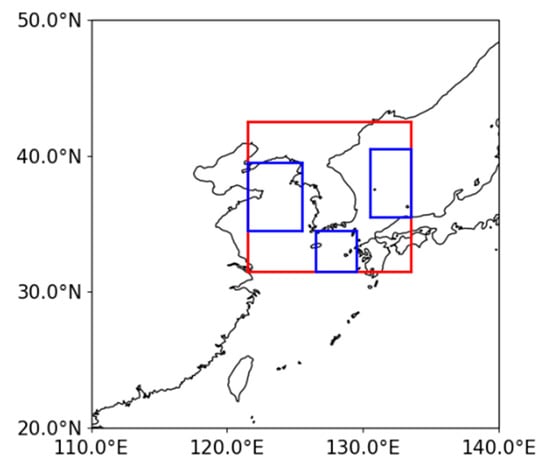
Figure 1.
Map of the analysis domain for East Asia (EA) region in this study. A red box indicates the Korean peninsula (KO) region, and blue boxes indicate East Sea (ES), West Sea (WS), and South Sea (SS), respectively.
2.2. Contributions to Mean Sea Level
Sea levels are affected by thermal expansion and contraction of the ocean water, caused by density changes due to temperature changes. The changes in land ice mass (glaciers and ice sheets) and groundwater storage also contribute to sea level. To estimate the 21st-century contributions to SLR, we have predominately used the data of eight contribution components recommended by the IPCC AR5 [29]. The SLR as a function of time t is expressed by Equation (1).
where SLR(t)ocean consists of ocean thermal expansion and density change to SLR. Thermal expansion is one of the major contributors to sea level changes and is the only component simulated directly from CMIP models [51]. We have used the CMIP6 variable “zostoga” provided by each CMIP6 modeling group, which represents the thermal expansion for the full depth of the oceans [66]. SLR(t)glaciers is the mass loss of glaciers change (include ice caps). This component is another major contributor [51,67] and is simulated by the volume-area approach [68] model developed by Slangen and Van de Wal [28]. The change of glaciers is estimated using CMIP6 projections of temperature change (ΔT) and precipitation change (ΔP), accounting for the change of glacier area (A) and time (t). Summer is June–August in Northern Hemisphere and December–February in Southern Hemisphere.
SLR(t) = SLR(t)ocean + SLR(t)glaciers + SLR(t)ice sheets + SLR(t)ground water + SLR(t)GIA
SLR(t)ice sheets refers to ice sheet contribution and is split into a surface mass balance (SMB) contribution and dynamical contribution. The ice sheet is a glacier larger than 50,000 km2 and is now present in Antarctica and Greenland. First, SMB is called surface mass change when ice sheets disappear or are created due to temperature, precipitation, etc. In this study, SMB contribution is derived by Slangen et al. [2] as the following equation:
ΔSMBAntartica = −0.0105 − 0.01759 × δTatm − 0.0412
ΔSMBGreenland = 0.0153 + 0.01493 × δTatm − 0.00094
These Equations (2) and (3) are considered the projected global mean surface temperature (δTatm) to calculate the SMB contribution of the ice sheets [69,70]. Second, the mechanisms for dynamic changes on the ice sheets are a little different between Antarctica and Greenland. On Antarctica, incoming solar energy melts the ice shelf and creates a water pool on the surface. This results in the thinning and breaking up of the ice shelf [71]. Ice shelves may also melt as the bottom balance is changed due to warmer water circulation [72]. On the contrary, the main mechanisms on Greenland are calving, melt of marine-terminating glaciers [73], and ice flow-SMB feedback [74]. In this study, the dynamical contribution is estimated by scaling the SMB values [75].
SLR(t)groundwater refers to land water storage (groundwater depletion) contribution. This component is based on the data from Wada et al. [52], which is estimated by a global hydrological model to calculate groundwater depletion using country-specific data (groundwater abstraction and recharge). We have used recent GIA results from ICE-5G(VM2) [76,77,78] for SLR(t)GIA. These components (SLR(t)groundwater and SLR(t)GIA) are obtained from the CMIP5 data [51] provided by the Integrated Climate Data Center (ICDC).
3. Results
3.1. Present Day Trend
Figure 2 shows the spatial mean time series of SLR and SST changes relative to the mean climatology of the PD period from observation and nine CMIP6 models. The global mean SLR and its observation trend (3.24 mm year−1) for the PD period are similar to those mentioned in the IPCC AR5 (3.2 ± 0.4 mm year−1; 1993–2010) [4,51]. The rate of increase in the GMSL has accelerated in recent decades due to increasing rates of ice loss in Greenland and Antarctic [79]. Similarly, the simulated global SLR trend for the PD period is 5.3 ± 2.9 mm year−1, exceeding the observed trend (Figure 2a). This appears to be related to a higher increasing trend of temperature from CMIP6 models. The CMIP6 models have high climate sensitivity, as the response to past global warming in the CMIP6 models tend to be large [55,56,57,58,59,60,61,62,63,64]. Global warming and SLR have a positive relation. Consequently, the SLR trend for the PD period from CMIP6 is greater than the observation due to the characteristics of the CMIP6 models. Greater detail on these factors requires further study.
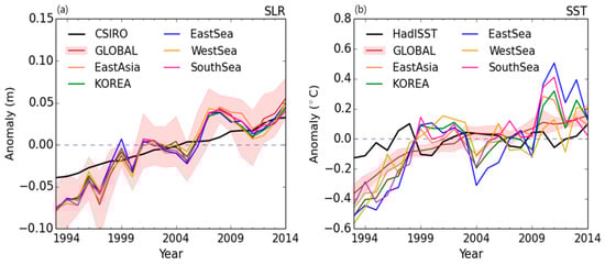
Figure 2.
Spatial mean time series of (a) Sea Level Rise (SLR; m) and (b) Sea Surface Temperature (SST; °C) anomalies from observation (black) and ensemble means of CMIP6 models for the global (dark red) with 95% confidence intervals (shaded), East Asia (coral), Korean peninsula (green), East Sea (blue), West Sea (yellow), and South Sea (pink) during the PD period. The reference is the mean climatology of the PD (1995~2014) period.
Regionally, the SLR trends in EA (5.3 ± 2.7 mm year−1) and KO (4.5 ± 2.9 mm year−1) are similar and lower than the global trends. Moreover, the SLR trends of local seas for the PD period are 4.2 ± 2.8 mm year−1, 4.3 ± 3.3 mm year−1, and 4.8 ± 2.9 mm year−1 in ES, WS, and SS, respectively. Particular years have recorded anomalously low SLR values (1996, 2000, 2005, and 2010) (Figure 2a). Several studies have reported that the sea level change around the KO tends to lower when the Kuroshio Current is strong [16,41].
The global SST trend in CMIP6 models for the PD period is 0.17 ± 0.06 °C per decade, more than three times the observation of 0.05 °C per decade (Figure 2b). In addition, the EA (0.20 ± 0.09 °C per decade) and KO regions (0.21 ± 0.25 °C per decade) show larger SST increases in the PD period. For the marginal seas around KO, the trend of ES (0.31 ± 0.39 °C per decade) is the highest. The EA and KO regions show more significant SST increases than the global region. However, the WS show the least significant trend (0.12 ± 0.21 °C per decade) in local seas (Figure 2b).
3.2. Future Projection
3.2.1. Global and East Asia Region
Compared to the PD period, Figure 3 shows the future changes in SLR and SST for the 21st century. The simulated projections have a similar positive trend until 2030. As mentioned in AR5, near-term projections are dependent on internal variability rather than the greenhouse gas (GHG) scenario [51]. In the LT period, rising trends and ensemble spreads are proportional to the concentration pathway of the scenarios. Bouttes and Gregory [80] report that these ranges are due to the spread of projected changes in ocean heat fluxes. This impact is visible in the SST increases in CMIP6 models after the 2030s. Therefore, on average, the projected range of global SST changes in the LT period relative to the PD period is expected to be 0.89 °C and 3.03 °C for SSP1-2.6 and SSP5-8.5, respectively. In addition, the SLR projection shows similar trends to the trend of SST warming, which is 0.28 m and 0.65 m for SSP1-2.6 and SSP5-8.5, respectively. The SSP1-2.6 result is smaller than that for Representative Concentration Pathway (RCP) 2.6 (0.41 m). However, the SSP5-8.5 projection is larger than RCP8.5 (0.63 m). In addition, the SLR difference between the SSP1-2.6 and SSP5-8.5 scenarios is approximately 0.37 m by the end of the century, exceeding the SLR difference between RCP 2.6 and RCP 8.5 (0.23 m; [51]). Global warming and GHG emissions are higher (lower) in SSP5-8.5 (SSP1-2.6) than in the RCP scenarios [45]. This indicates that the expected global warming is higher in the new CMIP6 scenario. Moreover, the SLR uncertainty spread for the two scenarios is 0.17–0.38 m (SSP1-2.6) and 0.52–0.78 m (SSP5-8.5). This spread range is smaller than that of CMIP5 (0.21–0.62 m for RCP 2.6 and 0.37–0.94 m for RCP 8.5; [29,59]). Additionally, the high bound of the spread for SSP1-2.6 (0.38 m) is smaller than the mean SLR of SSP5-8.5. This comparison demonstrates that the SLR is proportional to the concentration pathway of the scenarios. The SST change (1.10–3.54 °C) in the EA during the LT period is larger for both SSP scenarios than global. However, the SLR trend (0.28–0.67 m) is similar.
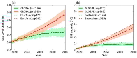
Figure 3.
Time series of (a) SLR and (b) SST anomalies in global (solid) and EA (dashed) for LT period (SSP1-2.6 (green) and SSP5-8.5 (red)) relative to PD period (1995–2014). The shading area indicates a 5–95% confidence range of global trend from nine CMIP6 models.
Figure 4 illustrates the spatial pattern of global mean SLR and SST changes in the LT period under the SSP1-2.6 and SSP5-8.5 scenarios. The ensemble mean of the SLR distribution (Figure 4a,b) shows typical features of the SLR response to CO2 emissions [26,27,30,32,80] and is affected by the global thermal expansion of the ocean in response to global warming [2]. Some of the large ranges of SLR (greater than 0.5 m) occurs in the southern Arctic Ocean, the dipole in the North Atlantic, and the meridional dipole in the Southern Oceans for both scenarios. In particular, in the SSP5-8.5 scenario, projected SLR exceeds 0.8 m in the meridional dipole in the Southern Oceans. These regions are associated with increasing GHGs [3,4,32] and westerly wind changes and wind-driven circulation changes [80]. Although the individual models disagree on the detailed spatial distribution and magnitude of the regional changes (particularly at high latitudes) due to differences in grid resolution and related processes, climate models show common global features in SLR [31]. Similarly, the CMIP6 simulations of the projected changes in SST for the 21st-century show typical patterns of the SST response to GHG emissions (Figure 4c,d) [44]. The positive anomalies occur in most domains, particularly in the northern mid to high latitudes. Alexander et al. [44] report that the absence of arctic sea-ice leads to an increasing trend of SST changes in high latitude regions (especially in summer). This trend is similar to the rising surface temperature in response to GHG emissions, indicating that SST is affected by the atmosphere-ocean interaction.
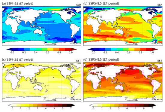
Figure 4.
Spatial distribution (global) of SLR (m; a,b) and SST (°C; c,d) anomalies from the ensemble mean of CMIP6 models for LT period relative to PD period.
3.2.2. Marginal Seas around the Korean Peninsula
Figure 5 displays the time series of the SLR and SST changes in the KO and surrounding local seas. Similar to global changes, the SLR and SST future projections until approximately 2030 are similar in both scenarios, and the increasing trend differs significantly after 2030. The projected SST change in SSP1-2.6 stabilizes after the mid-century. However, the increase continues (0.45 °C per decade) in SSP5-8.5. Moreover, the local sea increasing trends are 0.59 °C per decade, 0.59 °C per decade, and 0.49 °C per decade for the ES, WS, and SS, respectively. These trends are more significant than the global trend (0.39 °C per decade), indicating that the marginal seas around KO are more vulnerable in the LT period. Besides, the SLR projection for the KO shows similar trends to the SST warming and is expected to increase to 0.25 m (0.15–0.35 m) and 0.63 m (0.50–0.76 m) for SSP1-2.6 and SSP5-8.5, respectively. In SSP5-8.5, the projected SLR in local seas is expected to be 0.68 m, 0.61 m, and 0.66 m for the ES, WS, and SS, respectively. These SLR projections are larger than the global trend and are also larger than the previous CMIP5 projection (KO; 0.38–0.65 m; [29,59]). The SLR in the KO shows only a north–south gradient in CMIP5 models (not shown; [43]). However, CMIP6 models consider coastal lines for SLR projections (Figure 6a,b). Unlike the SLR distribution, the SST changes show a north–south gradient in the KO, and a more significant change occurs in the higher latitudes (Figure 6c,d).
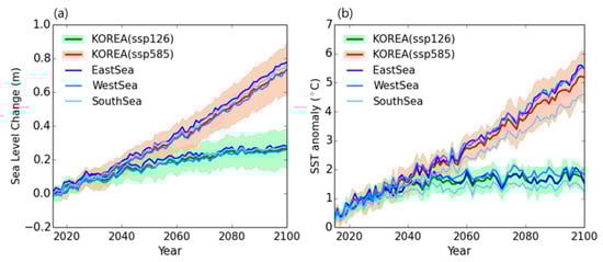
Figure 5.
Time series of (a) SLR (m) and (b) SST (°C) anomalies in KO (SSP1-2.6 (green) and SSP5-8.5 (red)), ES (dark blue), WS (blue), and SS (sky blue) for LT period relative to PD period. The shading indicates a 5–95% confidence range of KO trend from nine CMIP6 models.
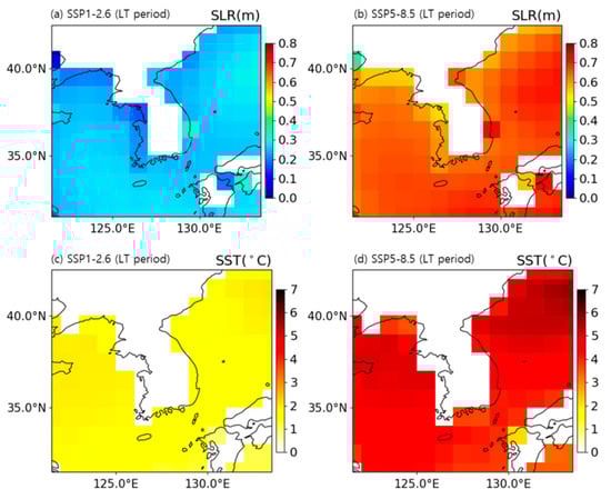
Figure 6.
Spatial distribution (KO) of SLR (m; a,b) and SST (°C; c,d) anomalies from the ensemble mean of CMIP6 models for the LT period relative to the PD period.
Figure 7 shows the simulated monthly SST changes in the local sea for the LT period. The trend’s median and 25th percentiles for SSP1-2.6 and SSP5-8.5 scenarios exceed 1 °C and 3 °C in all local seas. The SSP5-8.5 spread is significantly larger than that of SSP1-2.6. This suggests that the variation of SST projection is mainly due to differences between scenarios rather than internal variability. The local sea around the Korean peninsula is known to rise sharply due to the northward expansion of the Kuroshio Current, which is affected by global warming [38]. The Kuroshio Current is a warm current that transports tropical water northward toward the polar region. Therefore, the magnitude of the SST monthly change in both scenarios is greater during summer than during winter. In addition, the ES and WS show a larger seasonal cycle than the SS. This is a result of the channel-structure of the SS, and the Kuroshio Current moves toward the ES and the WS [39]. Overall, local current changes due to global warming predominantly affect the SST changes in KO.
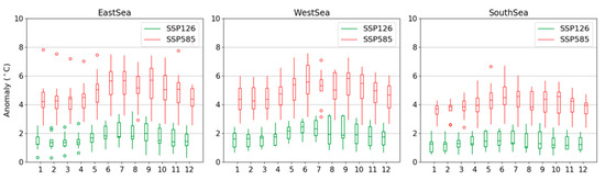
Figure 7.
Monthly mean SST trends from CMIP6 models in the LT period relative to the PD period. Green bars indicate SSP1-2.6, and red bars indicate SSP5-8.5. The x-axis means January to December.
For the SLR and SST projections, the most significant increase occurs in the ES compared to WS and SS. The ES is comprised of the deep sea (short continental shelf), and the coastal line stretches north and south. Therefore, the ES is significantly affected by ocean currents, such as the Liman Cold Current and the Kuroshio Warm Current [14,16,24,35,36,37,38,39]. If the ocean temperature increases due to global warming, the distribution of fish species will change, affecting the fisheries industry. Moreover, the negative effects of climate change will also significantly impact the dependent surrounding countries (i.e., South Korea, Japan, and Russia).
3.3. Contributions to 21st Century Sea Level Change
The future projected SLR in the LT period (Figure 4a,b) shows that SLR has not been spatially uniform and almost certainly accelerates in response to global warming [4,31]. At the end of the 21st century, SLR in 70% of the world’s coastal regions has shown a ±20% difference from the global mean values [10,51,79]. This difference in SLR is due to regional variations in factors, such as ocean thermal expansion and glacial melting [2,4,31,78]. To account for this response in qualitative analysis, we have compared the estimated SLR components from the climate model to three categories (ocean-related components, glacier components, and other components; Figure 8). The ocean-related components indicate dynamic sea level and thermal expansion terms, while the glacier components indicate glacier melting, ice sheet mass change (SMB), and dynamical ice sheet processes. In addition, the land water storage and GIA contribution are residual components. This method has been used in previous studies [29] to determine how quantitatively ocean-related processes or glacier melting due to global warming are related to SLR.
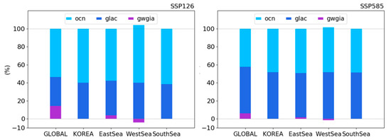
Figure 8.
Contributions of ocean-related components (ocn; sky-blue), glaciers (glac; blue), and other components (gwgia; purple) to SLR of LT period in the global, KO, and marginal seas around KO.
Ocean-related processes and glacier melting are major contributors to SLR in CMIP6 models, which have produced similar results to those of previous studies using CMIP5 models [2,4,31,78]. On a global scale, ocean-related components contribute to SLR by 54% and 42% for SSP1-2.6 and SSP5-8.5, respectively. In addition, glacier melting contributes 32% in SSP1-2.6 and 52% in SSP5-8.5. This indicates that glacier melting in CMIP6 models affects SLR more significantly than in CMIP5 models (15–35%). This difference may arise from CMIP6 models, predicting a higher degree of warming than CMIP5 models. In the ES, WS, and SS, the contribution of ocean-related components is 58–64% in SSP1-2.6 and 48–50% in SSP5-8.5, which is larger than their contribution to the global region. In addition, glacier melting is 38–40% in SSP1-2.6 and 49–52% in SSP5-8.5. This result implies that the proportion of ocean-related processes contributing to SLR decreases and glacier melting increases in higher emission scenarios. The difference in the contribution proportion between the averaged KO and local seas is approximately 2% in both scenarios. The smaller spread of each contribution in the higher emission scenario indicates that the component directly affected by temperature increase has a dominant impact on the SLR future projection rather [2,3,4,28,31] than individual regional contributions. Overall, this suggests that the impact of glacier melting is the main source of future sea level change.
4. Conclusions
Future SLR and SST changes are critical constraints on developments and population growth in coastal metropolitan cities [1,2,3,4,5,6,7,8]. Concerning global warming, the trend of SLR and SST changes is expected to steeply increase differently from the past, and this projection is particularly concerning for countries like Korea. This means that the coastal areas of the Korean peninsula are expected to be more vulnerable, and it will get serious in the 21st century. Thus, it is crucial to estimate future projections of SLR and SST changes to assess the mitigation and adaptation options within a sustainable development framework.
Considering this, we estimate future SLR and SST projections based on state-of-the-art nine CMIP6 participating models, including the K-ACE and UKESM1, which are performed by our research group [54,55,56,57,58,59,60,61,62,63,64]. To estimate future SLR in the 21st century, ocean-related and glacier components are considered. A total of eight contribution components are calculated using CMIP6 models following the recommended approach by the IPCC AR5 [29,66,67,68,69,70,71,72,73,74,75,76,77,78]. At first, global changes in SLR and SST are reconstructed for the past and projecting the future. For a more comprehensive analysis, we investigate regional projections and provide an understanding of the contributing components on a regional scale (KO region). Projections from SSP1-2.6 and SSP5-8.5 are used to estimate SLR and SST projections for the late 21st century (LT; 2081–2100). The results are summarized as follows.
- For the present-day period, the estimated global mean SLR trend is larger in CMIP6 simulations than in the observed. In the future, the trend is expected to be 0.28 m (0.17–0.38 m) and 0.65 m (0.52–0.78 m) for SSP1-2.6, SSP5-8.5, respectively. Spatially, there are significantly large changes over the Southern Ocean. Regional SLR of KO projects 0.25 m (0.15–0.35 m) and 0.63 m (0.50–0.76 m) for SSP1-2.6 and SSP5-8.5, respectively, which are similar to the global mean results. In the marginal seas around KO, projections in SSP5-8.5 are expected to increase to 0.68 m, 0.61 m, and 0.66 m for the ES, WS, and SS, respectively.
- Discrepancy between the global and regional changes is distinct in future SST warming rather than future SLR. Global mean SST is expected to rise to 0.39 °C per decade for SSP5-8.5, while the local trends are 0.59 °C per decade, 0.59 °C per decade, and 0.49 °C per decade for the ES, WS, and SS, respectively. These results are approximately 1.5 times greater than the global trend, indicating that marginal seas around KO are expected to be more vulnerable in the 21st century. In addition, seasonal change in summer is larger than in the winter.
- Ocean-related processes and glacier melting are major contributors to SLR in CMIP6 models. Glacier melting based on CMIP6 models (32–52%) is more significant than CMIP5 models (15–35%). In the local seas (ES, WS, and SS), the contribution of ocean-related components is 58–64% in SSP1-2.6 and 48–50% in SSP5-8.5, which is larger than their contribution to the global region. In addition, glacier melting is 38–40% in SSP1-2.6 and 49–52% in SSP5-8.5. This result implies that the proportion of ocean-related processes contributing to SLR decreases and glacier melting increases in higher emission scenarios.
Our point concerns the future projection of SLR and SST changes around KO based on new SSP scenarios for CMIP6. Considering the results from RCP scenarios in AR5, global SLR trends in this study are different, while the highest emission scenarios between SSP5-8.5 and RCP8.5 show similar magnitude at the end of the 21st century. The magnitude of future SLR is uncertain. For the uncertainty, limited representation in modeling is primarily reported [2,80]. To understand regional changes, it is necessary to consider the characteristic component for local SST changes. The SST around KO is known to rise sharply due to the northward expansion of the Kuroshio Current [14,16,24,35,36,37,38,39]. This is affected by climate change on an oceanic scale, such as Pacific Decadal Oscillation (PDO) [24,36,41,42] and El Niño-Southern Oscillation (ENSO) [36,40,81]. Therefore, the magnitude of the SST monthly change in both scenarios is greater during summer than during winter. Overall, SST changes in KO are predominately affected by local current changes due to global warming.
An analysis method to calculate SLR in this study is based on the AR recommendations. It could be applied in climate modeling communities to consider the projection changes due to reference periods and easy comparison with other studies. To overcome the limitations of the various modeling representation, an ensemble approach is used to reduce individual uncertainties [23]. A new phase of model experimentation (CMIP6) is in progress. We estimate the future projection of the CMIP6 multi-model ensemble for SLR in comparison to those of CMIP5 models [29] and update the previous analysis of Heo et al. [29]. The results of this study are able to provide new basic information about the future projection of the ocean ecosystem and to support the establishment of national climate change adaption policies.
Author Contributions
Conceptualization, H.M.S., K.-O.B. and J.-C.H.; Data curation, J.K. and J.-H.L.; Formal analysis, H.M.S., J.K. and S.S.; Investigation, J.-H.L., K.-O.B. and J.-C.H.; Methodology, H.M.S. and K.-O.B.; Resources, J.K.; Software, J.K. and J.-H.L.; Validation, J.K.; Visualization, J.K. and H.M.S.; Writing—original draft, H.M.S.; Writing—review & editing, H.M.S., S.S., K.-O.B. and J.-C.H.; Project administration, Y.-H.K.; Funding acquisition, Y.-H.K.; All authors have read and agreed to the published version of the manuscript.
Funding
This work was funded by the Korea Meteorological Administration Research and Development Program “Development and Assessment of IPCC AR6 Climate Change Scenarios” under Grant (KMA-2018-00321).
Institutional Review Board Statement
Not applicable.
Informed Consent Statement
Not applicable.
Data Availability Statement
The CMIP6 model results can be download from the ESGF node (https://esgf-node.llnl.gov/projects/cmip6).
Conflicts of Interest
The authors declare no conflict of interest.
References
- IPCC. Impacts, Adaptation, and Vulnerability Part B: Regional Aspects; Contribution of Working Group II to the Fifth Assessment Report of the Intergovernmental Panel on Climate Change; Barros, V.R., Field, C.B., Dokken, D.J., Mastrandrea, M.D., Mach, K.J., Bilir, T.E., Chatterjee, M., Ebi, K.L., Estrada, Y.O., Genova, R.C., et al., Eds.; Cambridge University Press: Cambridege, UK; New York, NY, USA, 2014. [Google Scholar]
- Slangen, A.B.A.; Carson, M.; Katsman, C.A.; van de Wal, R.S.W.; Köhl, A.; Vermeersen, L.L.A.; Stammer, D. Projecting twenty-first-century regional sea-level changes. Clim. Chang. 2014, 124, 317–332. [Google Scholar] [CrossRef]
- Slangen, A.B.A.; Meyssignac, B.; Agosta, C.; Champollion, N.; Church, J.A.; Fettweis, X.; Ligtenberg, S.R.M.; Marzeion, B.; Melet, A.; Palmer, M.D.; et al. Evaluating model simulations of twentieth-century sea level rise. Part 1: Global mean sea level change. J. Clim. 2017, 30, 8539–8563. [Google Scholar] [CrossRef]
- Church, J.A.; White, N.J. Sea-level rise from the late 19th to the early 21st century. Surv. Geophys. 2011, 32, 585–602. [Google Scholar] [CrossRef]
- Nicholls, R.J.; Cazenave, A. Sea-level rise and its impact on coastal zones. Science 2010, 328, 1517–1520. [Google Scholar] [CrossRef] [PubMed]
- Church, J.; Woodworth, P.L.; Aarup, T.; Wilson, S. Understanding Sea-Level Rise and Variability; Wiley: London, UK, 2010. [Google Scholar]
- Nicholls, R.J. Synthesis of vulnerability analysis studies. In Proceedings of WORLD COAST 1993; Coastal Zone Management Cetre: Rijkswaterstaat, The Netherlands, 1995; pp. 181–216. [Google Scholar]
- Cazenave, A.; Llovel, W. Contemporary sea level rise. Annu. Rev. Mar. Sci. 2010, 2, 145–173. [Google Scholar] [CrossRef]
- Martinez, M.L.; Intralawan, A.; Vazquez, G.; Perez-Maqueo, O.; Sutton, P.; Landgrave, R. The coasts of our world are of ecological, economic, and social importance. Ecol. Econ. 2007, 63, 254–272. [Google Scholar] [CrossRef]
- IPCC. Summary for Policymakers. In Climate Change 2013: The Physical Science Basis; Contribution of working group I to the fifth assess-ment report of IPCC the intergovernmental panel on climate change; Stocker, T.F., Qin, D., Plattner, G.-K., Tignor, M.M.B., Allen, S.K., Boschung, J., Nauels, A., Xia, Y., Bex, V., Midgley, P.M., Eds.; Cambridge University Press: Cambridege, UK; New York, NY, USA, 2014; pp. 3–29. [Google Scholar]
- Kang, Y.Q.; Moon, S.R.; Oh, N.S. Coastal and Harbour Engineering: Sea level rise at the southwestern coast. KSCE J. Civ. Eng. 2005, 25, 151–156. (In Korean) [Google Scholar]
- Kang, S.K.; Cherniawsky, J.Y.; Foreman, M.G.G.; Min, H.S.; Kim, C.H.; Kang, H.W. Patterns of recent sea level rise in the East/Japan sea from satellite altimetry and in situ data. J. Geophys. Res. 2005, 110, C07002. [Google Scholar] [CrossRef]
- Ha, K.J.; Jeong, G.Y.; Jang, S.R.; Kim, K.Y. Variation of the sea surface height around the Korean peninsula with the use of multi-satellite data and its association with sea surface temperature. Korean J. Remote Sens. 2006, 22, 519–531. (In Korean) [Google Scholar]
- Oh, S.M.; Kwon, S.J.; Moon, I.J.; Lee, E.I. Sea level rise due to global warming in the northwestern pacific and seas around the Korean peninsula. J. Korean Soc. Coast. Ocean Eng. 2011, 23, 236–247. (In Korean) [Google Scholar] [CrossRef][Green Version]
- Jeon, D.C. Relative sea-level change around the Korean peninsula. Ocean Polar Res. 2008, 30, 373–378. (In Korean) [Google Scholar] [CrossRef][Green Version]
- Yoon, J.J.; Kim, S.I. Analysis of long period sea level variation on tidal station around the korea peninsula. J. Korean Soc. Hazard Mitig. 2012, 12, 299–305. (In Korean) [Google Scholar] [CrossRef][Green Version]
- Jung, T.S. Change of mean sea level due to coastal development and climate change in the western coast of Korean peninsula. J. Korean Soc. Coast. Ocean Eng. 2014, 26, 120–130. (In Korean) [Google Scholar] [CrossRef]
- Choi, J.Y.; Kim, J.H. Study on Necessity of Creating New Sea City; Korea Maritime Institute: Busan, Korea, 2019. [Google Scholar]
- Cha, W.; Choi, J.; Lee, O.; Kim, S. Probabilistic Analysis of sea level rise in Korean major coastal regions under RCP 8.5 climate change scenario. J. Korean Soc. Hazard Mitig. 2016, 16, 389–396. [Google Scholar] [CrossRef]
- Lambeck, K.; Chappell, J. Sea level change through the last glacial cycle. Science 2001, 292, 679–686. [Google Scholar] [CrossRef]
- Hoffman, J.S.; Keyes, D.; Titus, J.G. Projecting Future Sea Level Rise: Methodology, Estimates to the Year 2100 and Research Needs; US Environmental Protection Agency: Washigton, DC, USA, 1983.
- Rahmstorf, S.; Cazenave, A.; Church, J.A.; Hansen, J.E.; Kelling, R.F.; Parker, D.E.; Somerville, R.C.J. Recent climate observations compared to projections. Science 2007, 316, 709. [Google Scholar] [CrossRef]
- Tebaldi, C.; Knutti, R. The use of the multi-model ensemble in probabilistic climate projections. Phil. Trans. R. Soc. A 2007, 365, 2053–2075. [Google Scholar] [CrossRef]
- Raper, S.C.B.; Cubasch, U. Emulation of the results from a coupled general circulation model using a simple climate model. Geophys. Res. Lett. 1996, 23, 1107–1110. [Google Scholar] [CrossRef]
- Yin, J.; Schlesinger, M.E.; Stouffer, R.J. Model projections of rapid sea-level rise on the northeast coast of the United States. Nat. Geosci. 2009, 2, 262–266. [Google Scholar] [CrossRef]
- Yin, J.; Griffies, S.M.; Stouffer, R.J. Spatial Variability of sea level rise in twenty first century projections. J. Clim. 2010, 23, 4585–4607. [Google Scholar] [CrossRef]
- Yin, J. Century to multi-century sea level rise projections from CMIP5 models. Geophys. Res. Lett. 2012, 39, 39. [Google Scholar] [CrossRef]
- Slangen, A.B.A.; van de Wal, R.S.W. An assessment of uncertainties in using volume area modeling for computing the twenty first century glacier contribution to sea level change. Cryosphere 2011, 5, 673–686. [Google Scholar] [CrossRef]
- Heo, T.-K.; Kim, Y.; Boo, K.-O.; Byun, Y.-H.; Cho, C. Future sea-level projections over the seas around Korea from CMIP6 simulations. Atmosphere 2018, 28, 25–35. [Google Scholar]
- Pardaens, A.K.; Lowe, J.A.; Brown, S.; Nicholls, R.J.; de Gusmao, D. Sea-level rise and impacts projections under a future scenario with large greenhouse gas emission reductions. Geophys. Res. Lett. 2011, 38, 38. [Google Scholar] [CrossRef]
- Meyssignac, B.; Slangen, A.B.A.; Melet, A.; Church, J.A.; Fettweis, X.; Marzeion, B.; Agosta, C.; Ligtenberg, S.R.M.; Spada, G.; Richter, K.; et al. Evaluating model simulations of twentieth century sea level rise. Part II: Regional sea-level changes. J. Clim. 2017, 30, 8565–8593. [Google Scholar] [CrossRef]
- Bilbao, R.A.F.; Gregory, J.M.; Bouttes, N. Analysis of the regional pattern of sea level change due to ocean dynamics and density changes for 1993-2099 in observations and CMIP5 AOGCMs. Clim. Dynam. 2015, 45, 2647–2666. [Google Scholar] [CrossRef]
- Kim, Y.; Goo, T.-Y.; Moon, H.; Choi, J.; Byun, Y.-H. Projection of future sea level change based on HadGEM2-AO due to ice sheet and glaciers. Atmosphere 2019, 29, 367–380. [Google Scholar]
- Lee, C.-E.; Kim, S.U.; Lee, Y.S. Estimation of the regional future sea level rise using long-term tidal data in the Korean peninsula. J. Korea Water Resour. Assoc. 2014, 47, 753–766. [Google Scholar] [CrossRef]
- Belkin, I.M. Rapid warming of large marine ecosystems. Prog. Oceanogr. 2009, 81, 207–213. [Google Scholar] [CrossRef]
- Hwang, J.D.; Suh, Y.S.; Ahn, J.S. Properties of sea surface temperature variations derived from NOAA satellite in North-eastern Asian Waters from 1990 to 2008. Korean J. Nat. Conserv. 2012, 6, 130–136. [Google Scholar]
- Hyun, J.-H.; Choi, K.-S.; Lee, K.-S.; Lee, S.H.; Kim, Y.K.; Kang, C.-K. Climate change and anthropogenic impact around the Korean coastal ecosystems: Korean Long-term Marine Ecological Research (K-LTMER). Estuaries Coasts 2020, 43, 441–448. [Google Scholar] [CrossRef]
- Wu, L.; Cai, W.; Zhang, L.; Nakamura, H.; Timmermann, A.; Joyce, T.; McPhaden, M.J.; Alexander, M.; Qiu, B.; Visbeck, M.; et al. Enhanced warming over the global subtropical western boundary currents. Nat. Clim. Chang. 2012, 2, 161–166. [Google Scholar] [CrossRef]
- Yeh, S.-W.; Kim, C.-H. Recent warming in the Yellow/East China Sea during winter and the associated atmospheric circulation. Cont. Shelf Res. 2010, 30, 1428–1434. [Google Scholar] [CrossRef]
- Nan, F.; Xue, H.; Yu, F. Kuroshio intrusion into the South China Sea: A review. Prog. Oceanogr. 2015, 137, 314–333. [Google Scholar] [CrossRef]
- Gordon, A.L.; Giulivi, C.F. Pacific decadal oscillation and sea level in the Japan/East Sea. Deep. Sea Res. Part I Oceanogr. Res. Papers 2004, 51, 653–663. [Google Scholar] [CrossRef]
- Min, H.S.; Kim, C.-H. Interannual variability and long-term trend of coastal sea surface temperature in Korea. Ocean Polar Res. 2006, 28, 415–423. (In Korean) [Google Scholar]
- Knutson, T.R.; Sirutis, J.J.; Vecchi, G.A.; Garner, S.; Zho, M.; Kim, H.-S.; Bender, M.; Tuleya, R.E.; Held, I.M.; Villarini, G. Dynamical downscaling projections of twenty-first-century atlantic hurricane activity: CMIP3 and CMIP5 model based scenario. J. Clim. 2013, 26, 6591–6617. [Google Scholar] [CrossRef]
- Alexander, M.A.; Scott, J.D.; Friedland, K.D.; Mills, K.E.; Nye, J.A.; Pershing, A.J.; Thomas, A.C. Projected sea surface temperatures over the 21st century: Changes in the mean, variability, and extremes for large marine ecosystem regions of northern oceans. Elem. Sci. Anth. 2018, 6, 9. [Google Scholar] [CrossRef]
- O’ Neill, B.C.; Tebaldi, C.; van Vuuren, D.P.; Eyring, V.; Friedlingstein, P.; Hurtt, G.; Knutti, R.; Kriegler, E.; Lamarque, J.-F.; Lowe, J.; et al. Scenario Model Intercomparison Project (ScenarioMIP) for CMip6. Geosci. Model Dev. 2016, 9, 3461–3482. [Google Scholar] [CrossRef]
- Eyring, V.; Bony, S.; Meehl, G.A.; Senior, C.A.; Stevens, B.; Stouffer, R.J.; Taylor, K.E. Overview of the Coupled Model Intercomparison Project Phase 6 (CMIP6) experimental design and organization. Geosci. Model Dev. 2016, 9, 1937–1958. [Google Scholar] [CrossRef]
- Thompson, P.R.; Hamlington, B.D.; Landerer, F.W.; Adhikari, S. Are long tide gauge records in the wrong place to measure global mean sea level rise? Geophys. Res. Lett. 2016, 43, 10403–10411. [Google Scholar] [CrossRef]
- Masters, D.; Nerem, R.S.; Choi, C.; Leuliette, E.; Beckley, B.; White, N.; Ablain, M. Comparison of Global Mean Sea Level Time Series From TOPEX/Poseidon, Jason-1, and Jason-2. Mar. Geod. 2012, 35, 20–41. [Google Scholar] [CrossRef]
- Henry, B.; Charmley, E.; Eckard, R.; Gaughan, J.B.; Hegarty, R. Livestock production in a changing climate: Adaptation and Mitigation Research in Australia. Crop Pasture Sci. 2012, 63, 191–202. [Google Scholar] [CrossRef]
- Tamisiea, M.E.; Mitrovia, J.X. The moving boundaries of sea level change: Understanding the origins of geographic variability. Oceanography 2011, 24, 24–39. [Google Scholar] [CrossRef]
- Wada, Y.; Bierkens, M.F.P.; de Roo, A.; Dirmeyer, P.A.; Famiglietti, J.S.; Hanasaki, N.; Konar, M.; Liu, J.; Schmied, H.M.; Oki, T.; et al. Human-water interface in hydrological modeling: Current status and future directions. Hydrol. Earth Syst. Sci. 2017, 21, 4169–4193. [Google Scholar] [CrossRef]
- Rayner, N.A.; Parker, D.E.; Horton, E.B.; Folland, C.K.; Alexander, V.; Rowell, D.P.; Kent, E.C.; Kaplan, A. Global analyses of sea surface temperature, sea ice, and night marine air temperature since the late nineteenth century. J. Geophys. Res. 2003, 108, 4407. [Google Scholar] [CrossRef]
- Lee, J.; Kim, J.; Sun, M.-A.; Kim, B.-H.; Moon, H.; Sung, H.M.; Kim, J.; Byun, Y.-H. Evaluation of the Korea Meteorological Administration Advanced Community Earth-system Model (K-ACE). Asia Pac. J. Atmos. Sci. 2020, 56, 381–395. [Google Scholar] [CrossRef]
- Sung, H.M.; Kim, J.; Shim, S.; Seo, J.; Kwon, S.-H.; Sun, M.-A.; Moon, H.; Lee, J.-H.; Lim, Y.-J.; Boo, K.-O.; et al. Evaluation of the NIMS/KMA CMIP6 model and future climate change scenarios based on new GHG concentration pathways. APJAS 2020. Accepted. [Google Scholar]
- Walters, D.; Baran, A.J.; Boutle, I.; Brooks, M.; Earnshaw, P.; Edwards, J.; Furtado, K.; Hill, P.G.; Lock, A.; Manners, J.; et al. The Met Office Unified Model Global Atmosphere 7.0/7.1 and JULES Global Land 7.0 configurations. Geosci. Model Dev. 2019, 12, 1909–1963. [Google Scholar] [CrossRef]
- Sellar, A.A.; Jones, C.G.; Mulcahy, J.P.; Tang, Y.; Yool, A.; Wiltshire, A.; O’ConnoriD, F.M.; Stringer, M.; Hill, R.; Palmieri, J.; et al. UKESM1: Description and evaluation of the U.K. Earth system model. J. Adv. Model. Earth Syst. 2019, 11, 4513–4558. [Google Scholar] [CrossRef]
- Ziehn, T.; Chamberlain, M.A.; Law, R.M.; Lenton, A.; Bodman, R.W.; Dix, M.; Stevens, L.; Wang, Y.-P.; Srbinovsky, J. Australian Earth System Model: ACCESS-ESM1.5. J. South Hemisph. Earth Sys. Sci. 2020, 193–214. [Google Scholar] [CrossRef]
- Swart, N.C.; Cole, J.N.S.; Kharin, V.V.; Lazare, M.; Scinocca, J.F.; Gillett, N.P.; Anstey, J.; Arora, V.; Christian, J.R.; Hanna, S.; et al. The Canadian Earth System Model version 5 (CanESM5). Geosci. Model Dev. 2019, 12, 4823–4873. [Google Scholar] [CrossRef]
- Wyser, K.; Kjellstrom, E.; Koenigk, T.; Martins, H.; Doscher, R. Warmer climate projections in EC-Earth3-Veg: The role of changes in greenhouse gas concentrations from CMIP5 to CMIP6. Envion. Res. Lett. 2020, 15, 054020. [Google Scholar] [CrossRef]
- Volodin, E.; Mortikov, E.V.; Kostrykin, S.V.; Galin, V.Y.; Lykossov, V.N.; Gritsun, A.S.; Diansky, N.A.; Gusev, A.V.; Iakovlev, N.G. Simulation of the present-day climate with the climate model INMCM5. Clim. Dyn. 2017, 49, 3715–3734. [Google Scholar] [CrossRef]
- Boucher, O.; Servonnat, J.; Albright, A.L.; Aumont, O.; Balkanski, Y.; Bastrikov, V.; Bekki, S.; Bonnet, R.; Bony, S.; Bopp, L.; et al. Presentation and evaluation of the IPSL-CM6A-LR climate model. J. Adv. Model. Earth Sys. 2020, 12. [Google Scholar] [CrossRef]
- Mauriten, T.; Bader, J.; Becker, T.; Behrens, J.; Bittner, M.; Brokopf, R.; Brovkin, V.; Claussen, M.; Crueger, T.; Esch, M.; et al. Developments in the MPI-M Earth System Model Version 1.2 (MPI-ESM1.2) and its response to increasing CO2. J. Adv. Model. Earth Syst. 2019, 11, 998–1038. [Google Scholar] [CrossRef]
- Yukimoto, S.; Kawai, H.; Koshiro, T.; Oshima, N.; Yoshida, K.; Urakawa, S.; Tsujino, H.; Deushi, M.; Tanaka, T.; Hosaka, M.; et al. The Meteorological Research Institute Earth System Model Version 2.0, MRI-ESM2.0: Description and basic evaluation of the physical component. J. Meteor. Soc. Jpn. 2019, 97, 931–965. [Google Scholar] [CrossRef]
- Williams, D.; Balaji, B.; Cinquini, L.; Denvil, S.; Duffy, D.; Evans, B.; Ferraro, R.; Hansen, R.; Lautenschlager, M.; Trenham, C. A global repository for planet-sized experiments and observations. Bull. Am. Meteorol. Soc. 2016, 97, 803–816. [Google Scholar] [CrossRef]
- Griffies, S.M.; Greatbatch, R.J. Physical processes that impact the evolution of global mean sea level in ocean climate models. Ocean Modell. 2012, 51, 37–72. [Google Scholar] [CrossRef]
- Marzeion, B.; Champollion, N.; Haeberli, W.; Langley, K.; Leclercq, P.; Paul, F. Observation based estimates of global glacier mass change and its contribution to sea-level change. Surv. Geophys. 2017, 38, 105–130. [Google Scholar] [CrossRef]
- Radic, V.; Hock, R. Regional and global volumes of glaciers derived from statistical upscaling of glacier inventory data. J. Geophys. Res. 2010. [Google Scholar] [CrossRef]
- Frezzotti, M.; Scarchilli, C.; Becagli, S.; Proposito, M.; Urbini, S. Synthesis of the Antarctic surface mass balance during the last 800 yr. Cryosphere 2013, 7, 303–319. [Google Scholar] [CrossRef]
- Fettweis, X.; Box, J.E.; Agosta, C.; Amory, C.; Kittel, C.; Lang, C.; Van As, D.; Machguth, H.; Gallée, H. Reconstructions of the 1900-2015 Greenland ice sheet surface mass balance using the regional climate MAR model. Cryosphere 2017, 11, 1015–1033. [Google Scholar] [CrossRef]
- Cook, A.J.; Vaughan, D.G. Overview of area changes of the ice shelves on the Antarctic Peninsula over the past 50 years. Cryosphere 2010, 4, 77–98. [Google Scholar] [CrossRef]
- Pritchard, H.D.; Ligtenberg, S.R.M.; Fricker, H.A.; Vaughan, D.G.; Broeke, M.R.V.D.; Padman, L. Antarctic ice sheet loss driven by basal melting of ice shelves. Nature 2012, 484, 502–505. [Google Scholar] [CrossRef] [PubMed]
- Nick, F.M.; Vieli, A.; Andersen, M.L.; Joughin, I.R.; Payne, A.; Edwards, T.L.; Pattyn, F.; Van De Wal, R.S.W. Future sea-level rise from Greenland’s main outlet glaciers in a warming climate. Nature 2010, 497, 235–238. [Google Scholar] [CrossRef] [PubMed]
- Goelzer, H.; Huybrechts, P.; Furst, J.J.; Nick, F.; Andersen, M.; Edwards, T.; Fettweis, X.; Payne, A.; Shannon, S. Sensitivity of Greenland ice sheet projections to model formulations. J. Glaciol. 2013, 59, 733–749. [Google Scholar] [CrossRef]
- Slangan, A.B.A.; Katsman, C.A.; van de Wal, R.S.W.; Vermeersen, L.L.A.; Riva, R.E.M. Towards regional projections of twenty-first century sea-level change based on IPCC SRES scenarios. Clim. Dyn. 2012, 38, 1191–1209. [Google Scholar] [CrossRef]
- Peltier, W.R. Global glacial isostasy and the surface of the ice-age earth: The ICE-5G(VM2) model and GRACE. Annu. Rev. Earth Planet Sci. 2004, 32, 111–149. [Google Scholar] [CrossRef]
- Frederikse, T.; Riva, R.E.M.; King, M.A. Ocean bottom deformation due to present-day mass redistribution and its impact on sea-level observations. Geophys. Res. Lett. 2017, 44, 12306–12314. [Google Scholar] [CrossRef]
- Martinec, Z.; Klemann, V.; Vander Wal, W.; Riva, R.E.; Spada, G.; Sun, Y.; Melini, D.; Kachuck, S.; Barletta, V.; Simon, K.; et al. A benchmark study of numerical implementations of the sea level equation in GIA modeling. Geophys. Res. Lett. 2018, 215, 389–414. [Google Scholar]
- IPCC. Special Report on the Ocean and Cryosphere in a Changing Climate; Portner, H.-O., Roberts, D.C., Masson-Delmotte, V., Zhai, P., Tignor, M., Poloczanska, E., Mintenbeck, K., Alegria, A., Nicolai, M., Lkem, A., et al., Eds.; Cambridge University Press: Cambridege, UK; New York, NY, USA, 2019; in press. [Google Scholar]
- Bouttes, N.; Gregory, J.M. Attribution of the spatial pattern of CO2 forced sea level change to ocean surface flux changes. Environ. Res. Lett. 2014, 9, 034004. [Google Scholar] [CrossRef]
- Little, C.M.; Horton, R.M.; Kopp, R.E.; Oppenheimer, M.; Yip, S. Uncertainty in twenty-first-century CMIP5 sea level projections. J. Clim. 2015, 28, 838–852. [Google Scholar] [CrossRef]
- Yoon, J.; Yeh, S.-W. Study of the Relationship between the East Asian marginal SST and the two different types of El Niño. Ocean Polar Res. 2009, 31, 51–61. [Google Scholar] [CrossRef]
Publisher’s Note: MDPI stays neutral with regard to jurisdictional claims in published maps and institutional affiliations. |
© 2021 by the authors. Licensee MDPI, Basel, Switzerland. This article is an open access article distributed under the terms and conditions of the Creative Commons Attribution (CC BY) license (http://creativecommons.org/licenses/by/4.0/).